Nov 9, 2017 - Preprint 10 November 2017. Compiled using MNRAS LATEX ... arXiv:1711.03252v1 [astro-ph.IM] 9 Nov 2017 .... 64 kernels. 1 x 5 convolution.
MNRAS 000, 000–000 (0000)
Preprint 10 November 2017
Compiled using MNRAS LATEX style file v3.0
Classifying Complex Faraday Spectra with Convolutional Neural Networks
arXiv:1711.03252v1 [astro-ph.IM] 9 Nov 2017
Shea Brown1? , Brandon Bergerud1 , Allison Costa1 , B. M. Gaensler2 , Jacob Isbell1 , Daniel LaRocca1 , Ray Norris3 , Cormac Purcell4 , Lawrence Rudnick5 , Xiaohui Sun6 1
Department of Physics & Astronomy, The University of Iowa, Iowa City, IA, 52245 Institute for Astronomy and Astrophysics, The University of Toronto, Toronto, ON M5S 3H4, Canada 3 Western Sydney University, Locked Bag 1797, 1797, Penrith South, NSW, Australia 4 Research Centre for Astronomy, Astrophysics, and Astrophotonics, Macquarie University, NSW 2109, Australia 5 Minnesota Institute for Astrophysics, University of Minnesota, 116 Church Street SE, Minneapolis, MN 55455, USA 6 Department of Astronomy, Yunnan University, and Key Laboratory of Astroparticle Physics of Yunnan Province, Kunming, 650091, China 2 Dunlap
ABSTRACT
Advances in radio spectro-polarimetry offer the possibility to disentangle complex regions where relativistic and thermal plasmas mix in the interstellar and intergalactic media. Recent work has shown that apparently simple Faraday Rotation Measure (RM) spectra can be generated by complex sources. This is true even when the distribution of RMs in the complex source greatly exceeds the errors associated with a single component fit to the peak of the Faraday spectrum. We present a convolutional neural network (CNN) that can differentiate between simple Faraday thin spectra and those that contain multiple or Faraday thick sources. We demonstrate that this CNN, trained for the upcoming Polarisation Sky Survey of the Universe’s Magnetism (POSSUM) early science observations, can identify two component sources 99% of the time, provided that the sources are separated in Faraday depth by >10% of the FWHM of the Faraday Point Spread Function, the polarized flux ratio of the sources is >0.1, and that the Signal-to-Noise radio (S/N) of the primary component is >5. With this S/N cut-off, the false positive rate (simple sources mis-classified as complex) is
Simple
Complex
P1 P2
1 [0, 1] [-50, +50] [0, +π] [0, 0.333]
True Simple True Complex
48,318 3,618
1481 46,583
φ{1,2} χ{1,2} σ
Table 3. Confusion Matrix: After Cutoffs
epochs, though no improvement on the validation set was found after 55 epochs. The weights found on epoch 55 were saved and used for testing.
4
RESULTS & DISCUSSION
The trained network was then applied to 100,000 new sources randomly generated using the same parameter space as the training set. The output for each source is a value p between 0 and 1 which can be thought of as the probability that the source is complex. Figure 5 shows a histogram of p for the 100,000 test sources. The distribution is bi-modal, indicating that the network was confident about the classification of most sources. If we take p > 0.5 as the threshold for complexity, we can construct the confusion matrix as shown in Table 2. The network produces 7.2% false negatives and 3.0% false positives. In order to hunt down the complex sources that are mis-classified as simple, we can plot the p for all the complex sources as a function of both the second component’s amplitude P2 and the absolute separation in the two components’ Faraday depths ∆φ = |φ1 − φ2 | (Fig. 6). The majority of false negatives happen at small P2 and ∆φ. This is consistent with the results of Farnsworth et al. (2011) and Sun et al. (2015) that point to the difficulty in identifying two component sources when ∆φ < F W HM of the Faraday Point Spread Function. Figure 7 shows an example of one of the false-negatives. For the purposes of constructing a classifier for largescale polarsation surveys like POSSUM, we would like to exclude the phase space of sources that would likely not make it into the catalog due to low signal-to-noise, as well as sources where the rotation measures of the two components are close enough to allow probing of a foreground Faraday screen. We therefore searched for the region of phase space in which we can detect >99% of the complex sources, allowing for the false positive rate to adjust appropriately based on the cut-off values. We found that if the minimum signalto-noise of the primary component is 5.0, and restrict our sample to P2 > 0.1, and ∆φ > 2.3 rad/m2 (which is about 10% of the 23 rad/m2 FWHM of the Faraday point spread function), the false negatives are reduced to