Classifying Data to Reduce Long Term Data Movement in Shingled Write Disks Stephanie N. Jones∗ , Ahmed Amer† , Ethan L. Miller∗ , Darrell D. E. Long∗ , Rekha Pitchumani∗ , Christina R. Strong∗ ∗ University
of California Santa Cruz {snjones, elm, darrell, rekhap, crstrong}@cs.ucsc.edu † Santa Clara University
[email protected] Abstract—Shingled Magnetic Recording (SMR) is a means of increasing the density of hard drives that brings a new set of challenges. Due to the nature of SMR disks, updating in place is not an option. Holes left by invalidated data can only be filled if the entire band is reclaimed, and a poor band compaction algorithm could result in spending a lot of time moving blocks over the lifetime of the device. We propose using write frequency to separate blocks to reduce data movement and develop a band compaction algorithm that implements this heuristic. We demonstrate how our algorithm results in improved data management, resulting in an up to 47% reduction in required data movements when compared to naive approaches to band management.
I.
I NTRODUCTION
Shingled Magnetic Recording (SMR) disks are devices that increase the storage density of traditional disk media by writing overlapping wide tracks of data, resulting in a shingle-like arrangement of the tracks. This presents us with a problem when overwriting previously written data, as it cannot be done without overwriting adjacent tracks. Overlapping tracks are therefore arranged into bands, and space reclamation is done at a band level. SMR disks therefore must employ band compaction to reclaim bands containing overwritten data, a concept similar to LFS cleaning. A number of bands are read in their entirety, and the valid blocks are compacted to a fewer number of bands, creating bands of free space. However, this can easily become expensive when the band compaction strategy is frequently moving data. We propose an algorithm for band compaction specifically designed to reduce long term data movement. The more time a shingled disk spends in band compaction, the more it is wasting resources. In the worst case, the system may need to block for I/O until band compaction completes making band compaction the bottleneck in the system and drastically reduces system responsiveness during that time. It is therefore necessary to develop band compaction strategies that mitigate the cost to the system. We claim that by separating blocks that are frequently updated from blocks that are less frequently (or never) updated, we can move fewer blocks in the long term. By applying this to band compaction, we have developed an algorithm that seeks to reduce long term data movement, potentially increasing the benefits of eliminating unnecessary activity and data movement in addition to reduc-
ing the overheads of employing SMR media. In order to reduce data movement, we are looking at using write heat as a metric to guide band compaction. For the purposes of this paper, write heat is measured in the frequency of writes to a LBA. By separating incoming write data based on write heat, we can reduce the likelihood of a band containing a mixture of hot and cold data. Bands that contain a mix of hot and cold data are more expensive to compact than bands that contain only hot or only cold data. In addition, having a large number of mixed bands can result in band compaction occurring at a higher frequency. For our purposes, we define data blocks to be “hot” if they have been overwritten at least once and “cold” otherwise. Bands that contain only cold data will be selected for compaction more frequently, and have more data that must be copied. Normally, this would cause concern but if the blocks are cold, they are expected to be long-lived and less likely to leave holes in a band. Bands that contain only hot data will be compacted less often, and will have less data needing to be copied per “hot” band. However, these blocks are volatile and are likely to be invalidated in the future leaving holes in the bands. Classifying data as hot or cold and placing it accordingly helps to reduce both the number of bands read before performing compaction as well as the overall amount of data copied during band compaction. There are currently three types of SMR disks: drivemanaged, host-managed, and host-aware) [1]. Drive-managed SMR disks present a block-based interface that is current used in non-shingled hard drives. It employs a Shingle Translation Layer to map the blocks to their particular band. A hostmanaged drive requires data sent to the drive to be written sequentially to its bands. Finally, a host-aware drive has bands that it prefers to receive sequential writes to but it also maintains an internal Shingle Translation Layer for any incoming non-sequential writes. The work presented in this paper is best suited for drive-managed SMR disks, but it can also work for host-aware and host-managed SMR disks. In order to simulate SMR disks, we implemented a log-structured file system (LFS) based translation layer with a block-based API. LFS segments and SMR bands are similar in concept, and band compaction in a SMR disk parallels segment cleaning in LFS. However, due to the unique properties of SMR disks, directly porting LFS is not feasible.
c 2015 IEEE 978-1-4673-7619-8/15/$31.00
Within this system, we replayed traces from the MSR Cambridge data set [2]. We applied our algorithm and compared it against a greedy algorithm that focuses on compacting the emptiest bands. Our algorithm gives priority to the emptiest bands, but also weights how much of the band is comprised of cold data when selecting bands for band compaction. We have found that the optimal value for the weight on cold varies depending on the workload. We have also identified several weight values that, while not optimal, provide a reduction in data movement. II.
R ELATED W ORK
A log-structuring of data, possibly through a log-structured file system or block remapping layer, seems suitable for SMR disks. However, in order for a LFS to work for SMR disks, data movement needs to be minimized, since writing to a band is not the same as writing to the log in the original LFS. Specifically, you can’t plug the holes in any of the bands and you can’t update in place. The goal of the original LFS was focused on creating large continuous spaces in which to write the log. This directly conflicts with our goal of maximizing the utilization of a band while minimizing data movement (thereby reducing the overall performance overhead of employing SMR disks). Since SMR technology was developed after the original LFS, there are characteristics of SMR disks which the original LFS can not fully utilize. Shingled disks may have a random access zone (RAZ) which can be used to hold metadata and other frequently modified data. Metadata updates in LFS are stored, like everything else, in the log. This can result in frequent holes in LFS segments, forcing cleaning to happen more often. Unless the segment is empty, segment cleaning results in data movement; an increase in cleaning is contradictory to our goal. A. Log-Structured File Systems and their Successors The log-structured file system (LFS) is a file system optimized for writing [3]. It assumes that main memory will satisfy more read requests as the size of main memory increases. This means that most requests that make it to disk will be write requests. LFS appends all modifications to on-disk data to the end of the log. By appending to the end of the log, LFS is able to maximize disk bandwidth for writing. The log is divided into segments, and a garbage collection policy is implemented to periodically clean the segments. LFS implements a cost-benefit policy for segment cleaning, shown in the formula below: cost free space generated × age of data = benefit cost The free space generated is measured by how much of the segment still contains live data. The age of the data is the age of the most recently modified block in the segment, meaning that heat is calculated on a per-segment basis. The cost of cleaning the segment is measured as the cost to read the segment plus the cost of writing the live data elsewhere. A problem with the cost-benefit policy is that if there is one recently modified block, but the rest of the data in the segment is very old, the age calculation can be misleading.
While a LFS segment and a SMR disk band are similar, our definition of heat is different. The original LFS makes two major assumptions: first, that heat is related to the recency of write; second, that blocks within a segment are written and modified together. We chose to begin by looking at heat as the frequency of a write to an LBA. This allows us to give data a value for heat that can later be changed with age, rather than a static “hot” or “cold” assignment. In addition, rather than considering heat on a segment basis, we calculate heat on a per-LBA basis. In this way, we can designate heat for specific logical locations and assign blocks to hot or cold bands as they are being written. BSD-LFS took the original design of LFS and modified it to work with UNIX FFS [4]. The authors evaluated BSDLFS using three workloads, the most notable of which was the TPCB benchmark. When testing BSD-LFS using the TPCB benchmark with 85% disk utilization, the cleaner was constantly running and copying large amounts of data into new segments. Blackwell et al. developed a simple heuristic to reduce the overhead found in BSD-LFS [5]. They showed that 97% of all cleaning in LFS during their tests could be done in the background. The authors used a simple heuristic of whether the disk had been idle for two seconds to signal that the segment cleaner should begin running. Such a technique is complimentary to our algorithm, and could be applied to SMR disks in order to compact fragmented bands in the background, rather than waiting for the disk to run out of free bands and compacting on demand. Matthews et al. demonstrated how to overcome the segment cleaning problem at higher disk utilizations [6]. They present an adaptive cleaning mechanism that chooses either full segment cleaning, as in LFS, or their technique of hole-plugging. Hole-plugging reads in segments to be cleaned and fills holes found in other segments with parts of the just-read segment. Traditional LFS segment cleaning provides the best performance until the disk utilization reaches 80-85%, at which point hole-plugging provides superior performance. It is important to note that, on a standard disk, the reason hole-plugging becomes better is because at 80-85% utilization, traditional LFS segment cleaning drops significantly in performance as shown in BSDLFS. Since hole-plugging is not generally usable in a SMR disks, with the possible exception of within the RAZ, this work is supplementary at best. PROFS is a data reorganization scheme that is aimed at improving I/O performance for log-structured file systems on drives with zone-bit recording (ZBR) technology [7]. It places “active” segments on the outer zones and inactive segments on the inner zones to optimize for faster writes. A segment’s active ratio is calculated using the average of the active ratio of each file in the segment. As in LFS, active is calculated by looking at recency of access, but PROFS also considers the size of the file and the last active ratio. The reorganization happens during LFS garbage collection. We will improve on the ideas behind PROFS by identifying hot and cold according to frequency at a block level, and place it accordingly as well as reorganize during band compaction. The closest LFS implementation to our work is the reordering Write buffer Of Log-structured File system, or WOLF [8]. WOLF sorts the incoming write data blocks into active and inactive data buffers, again using recency of access as the
metric for active. The sorting of data before it is written to disk is intended to reduce the overhead of the segment cleaner. WOLF follows Matthews’ proposed cleaning heuristic of combining the LFS cost-benefit policy with hole-plugging. In addition to using frequency of access as our metric, we continue to evaluate data during band compaction and place data in hot and cold bands appropriately.
Much of the research on SMR disks has focused on mitigating the “random update problem” [16], [17], [18], [19]. This is because due to the nature of SMR disks, random updates can not happen. This work is complementary to ours, as we don’t treat random updates any differently. Since band compaction is an inevitability, our work focuses on the proper selection of bands for compaction.
HyLog proposes a new type of hybrid log design to address LFS’s poor cleaning performance at high disk utilizations [9]. HyLog writes hot pages using standard LFS techniques, but writes cold pages in an “update-in-place” style which they call overwrite. Heat is measured on a per disk page basis, using frequency of write over an interval of time. Each disk page has a counter that is incremented every time it receives a write during the measurement interval. After this interval, the division of hot and cold pages occurs.
There has been some work on developing file systems for SMR drives [20], [21], which is also complimentary to our work. If we have semantic information from the file system, we can make better decisions on which bands have data that are likely to stay cool and which are likely to heat up. HiSMRfs [21] is capable of handling raw SMR drives, which would make providing information to the algorithms to select the proper bands for compaction more transparent.
Segment cleaning in HyLog is adapted from Matthews’ cleaning technique with a notable change: in Matthews’ work, the cleaning choices are either cost-benefit or hole-plugging and the ratios are calculated over every segment equally, but HyLog separates the ratios based on the heat of the segment. Specifically, HyLog compares the best ratio for hole-plugging over hot data, cost-benefit over hot data, hole-plugging for cold data, and cost-benefit for cold data. While this is effective for LFS, hole-plugging is not viable for SMR disks, nor is updating in place. There is often write contention found between the segment cleaner and the incoming data to be written. Gecko [10] solves this problem by chaining a small number of hard drives together into a single log. The tail of the log then is at a separate hard drive than the head of the log. By separating the head and tail of the log in this way, there is no longer write contention, as new data can be written to one drive while another is cleaning segments. B. Flash There is a rich body of work in the area of Flash storage that focuses on the separation of hot and cold data [11], [12]. However, some of the restrictions that apply to Flash and solid state drives can be ignored for SMR disks and vice versa [13] For instance, SMR disks do not care about wear leveling, nor is it necessary to zero a band before writing to it. In addition, bands can and will increasingly become much larger than a Flash page or erase block. When reading or writing data, there are seek penalties that must be considered for hard drives that do not exist for Flash. Therefore, any application of techniques borrowed from Flash would be in the spirit of their original work, and would not be likely to work as a direct port. C. Shingled Disk Amer et al. originally introduced the potential for SMR disks and the changes that would be required for their adoption [14]. Pitchumani et al. emulated a shingled write disk on a traditional hard drive. While informative, it is not necessary to fully emulate a shingled write disk to measure the reduction in data movement [15]. Skylight [1] was novel and drilled a hole into a SMR drive to understand how Seagate SMR drives work. This work will be instrumental in making decisions when testing our approach in the future.
III.
A LGORITHMS
In order to use shingled disks effectively we look at algorithms for reducing data movement during band compaction. Our approach is to look at the nature of the data blocks, classifying them appropriately. Techniques like this have been used in the past to produce self-optimizing data storage systems [22] and to reduce energy consumption of massive storage systems and devices [23]. To that end, we’ve developed a mechanism for classifying the hotness and coldness of data blocks which can be employed as part of the band compaction process. We compare our cold-weight algorithm against the more traditional baseline ranking that does not attempt to classify the blocks. A. Empty Empty is our greedy naive algorithm, which will always try to find an empty band. If there are no completely empty bands, empty will pick the bands with the least amount of live data to compact together. When compacting, empty will only find the number of bands it needs. For example, in 2-band compaction, empty will stop after finding the two bands with the least amount of live data; in 4-band compaction empty will stop after four. B. Cold-Weight The cold-weight algorithm combines a band’s freeness, or the amount of free space, with the heat (or the lack thereof) of the blocks contained within the band. The formula our algorithm uses to select bands is shown in Equation 1. F is the fraction of the band that is free; it is calculated as the number of dead blocks in a band divided by the number of blocks in the band. C is the fraction of the band that contains cold data; it is calculated as the number of cold blocks in a band divided by the number of blocks in a band. H is the fraction of the band that contains hot data; it is calculated as the number of hot blocks divided by the number of blocks in a band. These three variables will add up to 1: F + C + H = 1. wcold is the weight on cold and whot is the weight on hot. All variables, fractions, and weights are expressed in decimal form. F + (wcold × C) + (whot × H)
(1)
Where H, the hot fraction, can be measured in terms of free and cold. H =1−F −C (2)
C C C C C C
0.25 + 0.75 = 1.0
C H H H
0.5 + 0.125 = 0.625
C H
0.75 + 0.125 = 0.825
C C C C C C
0.25 + (0.75 × 0.5) = 0.625
C H H H
0.5 + (0.125 × 0.5) = 0.5625
C H
0.75 + (0.125 × 0.5) = 0.8125
(b) Cold-Weight
(a) Empty
Fig. 1: Example of why we need the weights in cold-weight. In Figure 1(a) we show the formula for cold-weight without the weight. Without the weight, it picks the segment that is 75% full of cold blocks. In Figure 1(b) we show that cold-weight in the same example with a weight of 50% will pick the band that is mostly empty with one cold and one hot block.
Thus, our algorithm can be simplified to look only at the free space and the cold data. Equation 3 contains the final form of the formula used by our algorithm to select bands for compaction and shows how everything can be represented as a weighted value on cold. In the derivation of Equation 3, the addition of the term whot is dropped because it is a constant value and does not change on a per-experiment basis. F + (wcold × C) + (whot × (1 − F − C)) F + (wcold × C) + whot − (whot × F ) − (whot × C) F × (1 − whot ) + C × (wcold − whot ) F +C ×(
wcold − whot ) 1 − whot
We use two traces from the MSR Cambridge data set that was introduced in FAST 2008 [2]. Specifically, we use the largest data volumes from the project (proj) and source code (src1) servers. The traces were gathered over a one week period, are block traces, and are stored on servers running NTFS. Table I shows some informative statistics about the traces we used. Both traces were chosen for their large number of write requests. We specifically chose the largest of the data volumes for the project and source servers from the MSR Cambridge traces because the data volumes will be more similar to a user workload than the traces of the system volumes.
(3)
The weight on cold can increase or decrease the importance of compacting bands that contain mostly cold data versus mostly hot data. For the workloads examined, we have found that a smaller weight on cold data produces the best results. Using the formula in Equation 3, we calculate a value for each band and select the bands with the highest values to use for compaction. Figure 1 shows why weighting is important. In Figure 1(a), we see that without weighting, we will pick the band with that is mostly full of cold blocks. This is because without weighting, we have assigned equal importance to cold blocks and free blocks. This is the point of putting the weight on cold blocks. In Figure 1(b), we use a weight of 50% on the percentage of the band that is cold. We pick the band that is mostly free with one cold and hot block. This is preferable because it’s better to take the chance on the single hot block than continuously move blocks from mostly full bands to new locations. IV.
A. Data Sets
E XPERIMENTAL S ETUP
In this section, we cover all of the components involved in running our experiments. We introduce the input data sets that were used to test the band compaction algorithms, and discuss the methods used to stress the algorithms. We also discuss a technique to better classify incoming blocks. Finally, we outline our code flow and describe all possible paths an incoming write block can take, along with the events that can be triggered. All of the experiments were kept in memory and “writing to disk” was simulated.
B. Pre-population Since the benefits of this technique should accumulate over time, we are interested in behavior over ever-longer periods of time and ever-larger data sets. To that end, in addition to studying the basic MSR traces, we extended the workloads by pre-populating our system with a random ordering of the same trace we would be playing. We cut the trace into chunks of 10 timesteps where a timestep is considered to be one second. This means that ten timesteps is at least 10 seconds, but could be longer if there is a period of inactivity in the trace. These chunks were randomly reordered and written out to a file. We chose to write it to a file because we can recreate the same on disk state for each run for fair comparison. We tested both algorithms without pre-population, pre-populating with a random selection of 50% of the writes in the trace, and prepopulating with a random ordering of all of the writes in each trace file. C. Write Buffer In order to model a more realistic workload we implemented a write buffer, which also afforded the opportunity to better classify incoming blocks as hot or cold. The size of the write buffer varies proportionally to the size of the band; it is always double the band size. When the write buffer is filled, it will pick an empty band to write out some of the data. If there is more hot data than cold data in the buffer, it will write out the hottest half of the data blocks. If there is more cold data than hot, the write buffer will write out the colder half of the data blocks. When there are no empty bands to write to, the write buffer will invoke band compaction. When band compaction completes, the write buffer will write out the half
TABLE I: Important statistics for the project and source control 1 servers. Number of Write Requests Total Data Written Trace Footprint Percentage of hot LBAs Percentage of cold LBAs Percentage of trace that is hot Percentage of trace that is cold
of the data with the more prevalent temperature until it fills the newly free band. D. Code Flow When a write request comes in, the request is divided into blocks. For each block written, a check is issued to see if it is already “on disk”. If it is, the heat of the block is incremented, and the current location on disk is marked as invalid. The block is then added to the write buffer. If it does not exist on disk, the block is marked as cold and immediately added to the write buffer. Currently, heat information is kept with the mapping of LBA to physical location in our simulation. In a real system, the heat information could be conveyed using a single bit in the shingle translation layer. When the write buffer is full, it selects a band to fill from any available empty bands. If there are no empty bands, the write buffer will invoke band compaction. Band compaction returns the location of a band to write to, and the write buffer fills the band with either the hottest or coldest data in the buffer as was described in Section IV-C. When the trace ends, band compaction is called as many times as necessary to flush the write buffer to disk. Currently, band compaction is only invoked in these two situations, and in both situations it is invoked by the write buffer. When band compaction is invoked, the first step is to calculate values for each of the bands in the system using one of the algorithms described in Section III-B. The bands with the highest values are selected based on however many bands are being compacted. As mentioned previously, the entire band has to be read, so all live data is read from the selected bands and sorted by their current write heat. At this point, a cooling step occurs: all of the heat counters are reset, making all of the data previously read cold. This is the only point at which data cooling currently happens. All of the bands that were read from are now marked as empty and are free to use. The live blocks that were read are written back to a free band. If we fill up the band before running out of live blocks, another recently freed band is selected and writing continues. When all live blocks have been written back to disk, the band that is currently being written to is the one that will receive future writes. In the case where the last block we wrote to is the last location in a band, another band is selected from the set of recently freed bands. V.
R ESULTS
We tested weights on cold in our cold-weight algorithm in 10% increments. These weights yielded both positive and negative results. We have chosen to present the results that demonstrate the optimal weights for both the empty algorithm
Project 2,496,935 26 GB 9.5 GB 20.45% 79.55% 64.68% 35.32%
Source 1 2,170,271 31 GB 4.4 GB 19.45% 81.55% 88.81% 11.19%
and the cold-weight algorithm for the sake of brevity. Table II shows the optimal improvement for each of the runs using a band size of 40MB. The results for a band size of 80MB are similar, and have been omitted due to space constraints. For a band size of 40MB, the project data set experiments use 279 total bands, and the source data set experiments use 128 bands. In any band, there can be hot, cold, and free blocks. In addition to moving fewer bands during band compaction, we also want to minimize the number of bands that have a mix of all three types of blocks, as this will give us a better separation of hot and cold blocks. The graphs show the number of blocks in each band that are hot (in red), cold (in blue), and free (in green); the bands are then sorted by heat. A. No Pre-population Figures 2 and 3 show the distribution of hot and cold blocks over all the bands in the experiments that were run without prepopulation. Due to the write buffer discussed in Section IV-C, we achieve a very good separation of hot and cold data. 1) Project: Figure 2 shows the project data set experiments. In both the empty and cold-weight experiments, the write buffer kept the number of bands with a mix of hot, cold and free blocks under 20. As seen in Table II, using cold-weight with a 30% weight produced the best reduction in data movement, a 12% improvement over empty. 2) Source: Figure 3 shows the source data set experiments. In these experiments, the number of bands with a mix of blocks was kept under 10 by the write buffer. It is interesting to note that for this workload, the optimal weight for the cold-weight algorithm was 50%, producing close to 3% improvement. B. 50% Pre-population We use a random selection of 50% of the write requests to pre-populate the system, as described in Section IV-B. Since we are using the same trace data to pre-populate the system as we are to run the experiments and cooling only happens during band compaction. Therefore, more hot blocks at the end of the trace means that less data was moved. 1) Project: Figure 4 shows the distribution of hot and cold blocks for all the bands in the project experiments. As can been seen in the graphs, there is more hot data left by the cold-weight algorithm than by the empty algorithm. This is illustrated in Table II, where a 10% weight on cold shows a 4% improvement in reducing data movement. Additionally, for this workload cold-weight does a better job of separating hot and cold data, leaving only 27 bands that have a mix of hot, cold, and free compared to empty’s 38 bands.
80000
Project 40MB Bands - Empty - 0% Pre-population
Project 40MB Bands - Cold Weight of 30% - 0% Pre-population 80000 70000 Composition of Blocks in Band
Composition of Blocks in Band
70000 60000 50000 40000 30000 20000 10000 00
hot cold free 50
60000 50000 40000 30000 20000 10000
100 150 200 Distribution of Bands
250
00
300
hot cold green 50
100 150 200 Distribution of Bands
250
300
Fig. 2: Comparison of the Empty and Cold-Weight algorithms for project without pre-population using 40MB bands. Green represents free blocks, blue represents cold blocks, and red represents hot blocks.
80000
Source1 40MB Bands - Empty - 0% Pre-population
Source1 40MB Bands - Cold Weight of 50% - 0% Pre-population 80000 70000 Composition of Blocks in Band
Composition of Blocks in Band
70000 60000 50000 40000 30000 20000 10000 00
hot cold free 20
60000 50000 40000 30000 20000 10000
40
60 80 100 Distribution of Bands
120
00
140
hot cold green 20
40
60 80 100 Distribution of Bands
120
140
Fig. 3: Comparison of the Empty and Cold-Weight algorithms for Source 1 without pre-population using 40MB bands. Green represents free blocks, blue represents cold blocks, and red represents hot blocks.
80000
Project 40MB Bands - Empty - 50% Pre-population
Project 40MB Bands - Cold Weight of 20% - 50% Pre-population 80000 70000 Composition of Blocks in Band
Composition of Blocks in Band
70000 60000 50000 40000 30000 20000
hot cold free
10000 00
50
100 150 200 Distribution of Bands
250
60000 50000 40000 30000 20000
hot cold green
10000 300
00
50
100 150 200 Distribution of Bands
250
300
Fig. 4: Comparison of the Empty and Cold-Weight algorithms for project with 50% pre-population using 40MB bands. Green represents free blocks, blue represents cold blocks, and red represents hot blocks.
TABLE II: The optimal weights of cold-weight when compared to empty for the 40MB band experiments with different levels of pre-population and different workloads. No Pre-population Experiment Blocks Moved Empty Project 40MB 2378357 Cold-Weight Project 40MB-30% weight 2082264 Empty Source 1 40MB 318607 Cold-Weight Source 1 40MB-50% weight 310262 50% Pre-population Empty Project 40MB 71568329 Cold-Weight Project 40MB-20% weight 68478899 Empty Source 1 40MB 1608014 Cold-Weight Source 1 40MB-40% weight 1548803 100% Pre-population Empty Project 40MB 72702645 Cold-Weight Project 40MB-10% weight 66031282 Empty Source 1 40MB 45122495 Cold-Weight Source 1 40MB-50% weight 23830466
80000
Source1 40MB Bands - Empty - 50% Pre-population
— 9.18% — 47.19%
70000 Composition of Blocks in Band
Composition of Blocks in Band
— 4.32% — 3.68%
Source1 40MB Bands - Cold Weight of 40% - 50% Pre-population 80000
70000 60000 50000 40000 30000 20000
hot cold free
10000 00
Percentage Improvement — 12.45% — 2.62%
20
40
60 80 100 Distribution of Bands
120
60000 50000 40000 30000 20000
hot cold green
10000 140
00
20
40
60 80 100 Distribution of Bands
120
140
Fig. 5: Comparison of the Empty and Cold-Weight algorithms for Source 1 with 50% pre-population using 40MB bands. Green represents free blocks, blue represents cold blocks, and red represents hot blocks.
2) Source1: Figure 5 shows the results of the source experiments. Interestingly, both cold-weight and empty have 11 bands remaining with a mix of hot, cold and free blocks. In the cold-weight experiment, there is about one band’s worth of extra hot blocks compared to empty. This means that most of the segments with cold data were mostly full, so we were selecting mostly empty segments with hot data and cooling them. Table II shows that with a 40% weight, cold-weight shows an almost 4% improvement. C. 100% Pre-population As in the experiments with 50% pre-population, more hot data at the end of the trace (as shown in the graphs) means we are touching less data during the course of the experiment. We are pre-populating the system with 100% of the write requests from the same trace data, in random order. 1) Project: The results of the project experiments are very similar to the results with 50% pre-population. As can be seen in Figure 6, there is more hot data remaining with the coldweight algorithm, reflected in the 9% improvement shown in Table II. Cold-weight also does a better job of separating hot and cold data, ending with 26 bands of mixed blocks compared to empty’s 32 bands. 2) Source1: The source experiments with 100% prepopulation showed the greatest improvement in reducing data
movement, at 50% weight for our cold-weight algorithm. Figure 7 shows the difference in the amount of hot data left with cold-weight versus empty. Cold-weight with a weight of 50% results in a 47% improvement in reducing data movement. While there are more bands with a mix of hot, cold, and free blocks (19 bands in cold-weight versus 13 in empty), it is most likely due to the behavior of the write buffer. Toward the end of the trace, the write buffer wrote hot data to a recently compacted band, resulting in mixed data. We will address this behavior in future work. VI.
F UTURE W ORK
The work presented here is only the beginning of our work to develop techniques to reduce data movement in storage systems and evaluate their usefulness to SMR disks and their applications. The next immediate step is to explore pre-populating with different percentages beyond 50 and 100, in order to obtain additional data points. Additional data points will help inform more future work and will also further demonstrate the success of our work. In addition, we will implement LFS’s cost-benefit policy as a band compaction algorithm and compare it to our cold-weight algorithm. We hypothesize that the bands containing a mix of hot and cold blocks can be further reduced by modifying the band compaction algorithm, as well as improving how the write buffer flushes data. The write buffer can keep track of distinct
80000
Project 40MB Bands - Empty - 100% Pre-population
Project 40MB Bands - Cold Weight of 10% - 100% Pre-population 80000 70000 Composition of Blocks in Band
Composition of Blocks in Band
70000 60000 50000 40000 30000 20000
hot cold free
10000 00
50
100 150 200 Distribution of Bands
250
60000 50000 40000 30000 20000
hot cold green
10000 00
300
50
100 150 200 Distribution of Bands
250
300
80000 Source1 40MB Bands - Empty - 100% Pre-population
Source1 80000 40MB Bands - Cold Weight of 50% - 100% Pre-population
70000
70000 Composition of Blocks in Band
Composition of Blocks in Band
Fig. 6: Comparison of the Empty and Cold-Weight algorithms for project with 100% pre-population using 40MB bands. Green represents free blocks, blue represents cold blocks, and red represents hot blocks.
60000 50000 40000 30000 20000
hot cold free
10000 00
20
40
60 80 100 Distribution of Bands
120
60000 50000 40000 30000 20000
hot cold green
10000 140
00
20
40
60 80 100 Distribution of Bands
120
140
Fig. 7: Comparison of the Empty and Cold-Weight algorithms for Source 1 with 100% pre-population using 40MB bands. Green represents free blocks, blue represents cold blocks, and red represents hot blocks.
hot and cold bands, and maintain this distinction when writing data out. The band compaction algorithm then can be modified to take advantage of these distinct hot and cold bands during band compaction. All compacted blocks will be written to the cold band, and a third band will be introduced to represent blocks that “were once hot”, or were hot in the write buffer. We will investigate other metrics beyond write frequency to reduce data movement in SMR disks. The last element in this stage of our work is to develop a dynamic band compaction algorithm that automatically tunes the values of the weights. Since workloads can, and often do, change behavior over their lifetime, it is necessary to be able to adjust the band compaction algorithm as needed in order to obtain the best performance. In this paper, we introduced our work and discussed the benefits that it will have for shingled drives. Skylight [1] has demonstrated that Seagate’s shingled drives don’t use LFSstyle compaction to reclaim space, but it is possible that other drive manufacturers will use LFS-style compaction. We will also expand on how to adapt this work for host-managed and host-aware drives. The techniques presented in this paper aren’t limited by the storage media. They can be employed to reduce data movement on any storage media that employs a LFS approach to storing data.
VII.
C ONCLUSIONS
Since band compaction is a necessity for SMR disks, it is clear that improved algorithms are needed. In this paper, we proposed using write frequency as a metric to separate blocks in order to reduce data movement. We presented a band compaction algorithm we developed that implements this heuristic, and showed that our algorithm results in up to a 47% reduction in required data movements when compared to naive approaches. Our algorithm cold-weight favors the selection of the emptiest bands, but also weights how much of the band is comprised of cold data when selecting bands to compact. We found that the optimal value for the weight on cold varies depending on the workload. However, there is always a weight that produces an improvement in reducing data movement. We also have shown that using a write buffer provides excellent separation of hot and cold data. We conclude that write frequency is a valid and useful metric when used in a band compaction algorithm such as our cold-weight algorithm. This kind of algorithm, combined with a write buffer, reduces the amount of data moved over the lifetime of a workload.
VIII.
ACKNOWLEDGEMENTS
This work is supported in part by the National Science Foundation under award IIP-1266400 and industrial members of the Center for Research in Storage Systems. A. Amer and D. D. E. Long were supported in part by the National Science Foundation under awards CCF-1219163 and CCF1217648, by the Department of Energy under award DE-FC0210ER26017/DE-SC0005417, by the industrial members of the Storage Systems Research Center and by a gift from Wells Fargo. The authors would also like to thank the students of the Storage Systems Research Center for their suggested edits to this paper. R EFERENCES [1]
[2]
[3]
[4]
[5]
[6]
[7]
[8]
[9]
[10]
[11] [12]
[13]
[14]
[15]
A. Aghayev and P. Desnoyers, “Skylight-a window on shingled disk operation,” in Proceedings of the 13th USENIX Conference on File and Storage Technologies. USENIX, Feb. 2015, pp. 135–149. D. Narayanan, A. Donnelly, and A. Rowstron, “Write off-loading: practical power management for enterprise storage,” in Proceedings of the 6th USENIX Conference on File and Storage Technologies. USENIX Association, 2008, p. 17. M. Rosenblum and J. K. Ousterhout, “The design and implementation of a log-structured file system,” in ACM Transactions on Computer Systems, February 1992. M. Seltzer, K. Bostic, M. K. McKusick, and C. Staelin, “An implementation of a log-structured file system for UNIX,” in Proceedings of the Winter 1993 USENIX Technical Conference, January 1993, pp. 307–326. T. Blackwell, J. Harris, and M. Seltzer, “Heuristic cleaning algorithms in log-strucutred file systems,” in Proceedings of the Winter 1995 USENIX Technical Conference, January 1995. J. N. Matthews, D. Roselli, A. M. Costello, R. Y. Wang, and T. E. Anderson, “Improving the performance of log-structured file systems with adaptive methods,” in Proceedings of the 16th ACM Symposium on Operating Systems Principles (SOSP ’97), October 1997, pp. 238– 251. J. Wang and Y. Hu, “PROFS-performance oriented data reorganization for log-structured file system on multi-zone disks,” in Proceedings of the 9th International Symposium on Modeling, Analysis, and Simulation of Computer and Telecommunication Systems (MASCOTS ’01), 2001. ——, “WOLF-a novel reordering write buffer to boost the performance of log-structured file systems,” in Proceedings of the 1st Conference on File and Storage Technologies (FAST ’02), January 2002, pp. 47–60. W. Wang, Y. Zhao, and R. Bunt, “HyLog: A high performance approach to managing disk layout,” in Proceedings of the 3rd USENIX Conference on File and Storage Sytems (FAST ’04), February 2004, pp. 145–158. J.-Y. Shin, M. Balakrishnan, T. Marian, and H. Weatherspoon, “Gecko: contention-oblivious disk arrays for cloud storage.” in Proceedings of the 11th USENIX Conference on File an Storage Technologies, 2013, pp. 285–298. P. Desnoyers, “Analytic models of ssd write performance,” ACM Transactions on Storage (TOS), vol. 10, no. 2, p. 8, 2014. J.-W. Hsieh, T.-W. Kuo, and L.-P. Chang, “Efficient identification of hot data for flash memory storage systems,” in ACM Transactions on Storage, February 2006. P. Desnoyers, “What systems researchers need to know about nand flash,” in the 5th USENIX Workshop on Hot Topics in File and Storage Technologies (HotStorage’13), San Jose, California, 2013. A. Amer, D. D. Long, E. L. Miller, J.-F. Paris, and S. T. Schwarz, “Design issues for a shingled write disk system,” in 2010 IEEE 26th Symposium on Mass Storage Systems and Technologies (MSST). IEEE, 2010, pp. 1–12. R. Pitchumani, A. Hospodor, A. Amer, Y. Kang, E. L. Miller, and D. D. E. Long, “Emulating a shingled write disk,” in Proceedings of the 20th IEEE International Symposium on Modeling, Analysis, and Simulation of Computer and Telecommunication Systems (MASCOTS 2012), Aug. 2012.
[16]
[17]
[18]
[19]
[20]
[21]
[22]
[23]
[24]
[25]
[26]
D. Hall, J. H. Marcos, and J. D. Coker, “Data handling algorithms for autonomous shingled magnetic recording hdds,” Magnetics, IEEE Transactions on, vol. 48, no. 5, pp. 1777–1781, 2012. W. He and D. H. Du, “Novel address mappings for shingled write disks,” in Proceedings of the 6th USENIX conference on Hot Topics in Storage and File Systems. USENIX Association, 2014, pp. 5–5. Y. Cassuto, M. A. Sanvido, C. Guyot, D. R. Hall, and Z. Z. Bandic, “Indirection systems for shingled-recording disk drives,” in 2010 IEEE 26th Symposium on Mass Storage Systems and Technologies (MSST). IEEE, 2010, pp. 1–14. C.-I. Lin, D. Park, W. He, and D. Du, “H-SWD: Incorporating hot data identification into shingled write disks,” in Proceedings of the 20th IEEE International Symposium on Modeling, Analysis and Simulations of Computer and Telecommunication Systems (MASCOTS 2012), August 2012, pp. 248–255. D. Le Moal, Z. Bandic, and C. Guyot, “Shingled file system hostside management of shingled magnetic recording disks,” in Consumer Electronics (ICCE), 2012 IEEE International Conference on. IEEE, 2012, pp. 425–426. C. Jin, W.-Y. Xi, Z.-Y. Ching, F. Huo, and C.-T. Lim, “HiSMRfs: A high performance file system for shingled storage array,” in 2014 30th Symposium on Mass Storage Systems and Technologies (MSST). IEEE, 2014, pp. 1–6. M. Bhadkamkar, J. Guerra, L. Useche, S. Burnett, J. Liptak, R. Rangaswami, and V. Hristidis, “BORG: Block-reorganization for selfoptimizing storage systems,” in Proceedings of the 7th USENIX Conference on File and Storage Technologies (FAST ’09), February 2009. D. Essary and A. Amer, “Predictive data grouping: Defining the bounds of energy and latency reduction through predictive data grouping and replication,” ACM Transactions on Storage (TOS), vol. 4, no. 1, p. 2, 2008. Q. M. Le, K. SathyanarayanaRaju, A. Amer, and J. Holliday, “Workload impact on shingled write disks: All-writes can be alright,” in 2011 IEEE 19th International Symposium on Modeling, Analysis & Simulation of Computer and Telecommunication Systems (MASCOTS). IEEE, 2011, pp. 444–446. M. Sivathanu, V. Prabhakaran, F. I. Popovici, T. E. Denehy, A. C. Arpaci-Dusseau, and R. H. Arpaci-Dusseau, “Semantically-smart disk systems,” in Proceedings of the 2nd USENIX Conference on File and Storage Systems, April 2003, pp. 73–88. R. Y. Wang, T. E. Anderson, and D. A. Patterson, “Virtual log based file systems for a programmable disk,” in Proceedings of the 3rd Symposium on Operating Systems Design and Implementation (OSDI ’99), February 1999, pp. 29–43.