Classifying Dynamic Objects: An Unsupervised Learning Approach

Classifying Dynamic Objects: An Unsupervised Learning Approach Matthias Luber

Kai O. Arras

Christian Plagemann

Wolfram Burgard

Albert-Ludwigs-University Freiburg, Department for Computer Science, 79110 Freiburg, Germany {luber, arras, plagem, burgard}@informatik.uni-freiburg.de Abstract— For robots operating in real-world environments, the ability to deal with dynamic entities such as humans, animals, vehicles, or other robots is of fundamental importance. The variability of dynamic objects, however, is large in general, which makes it hard to manually design suitable models for their appearance and dynamics. In this paper, we present an unsupervised learning approach to this model-building problem. We describe an exemplar-based model for representing the time-varying appearance of objects in planar laser scans as well as a clustering procedure that builds a set of object classes from given training sequences. Extensive experiments in real environments demonstrate that our system is able to autonomously learn useful models for, e.g., pedestrians, skaters, or cyclists without being provided with external class information.

I. Introduction The problem of tracking dynamic objects and modeling their time-varying appearance has been studied extensively in robotics, engineering, the computer vision community, and other areas. The problem is hard as the appearance of objects is ambiguous, partly occluded, may vary quickly over time, and is perceived via a highdimensional measurement space. On the other hand, the problem is highly relevant in practice, especially in future applications for mobile robots and intelligent cars. Consider, for example, a service robot deployed in a populated environment, e.g., a pedestrian precinct. A number of tasks such as collision-free navigation or interaction require the ability to recognize, distinguish, and track moving objects including reliable estimates of object classes like ’adult’, ’infant’, ’car’, ’dog’, etc. In this paper, we consider the problem of detecting, tracking, and classifying moving objects in sequences of planar range scans acquired by a laser sensor. We present an exemplar-based model for representing the time-varying appearance of moving objects as well as a clustering procedure that builds a set of object classes from given training sequences in conjunction with a Bayes filtering scheme for classification. The proposed system, which has been implemented and tested on a real robot, does not require labeled object trajectories, but rather uses an unsupervised clustering scheme to automatically build appropriate class assignments. By pre-processing the sensor stream using state-of-the-art feature detection and tracking algorithms, we achieve a system that is able to

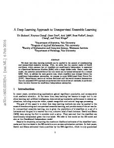
Fig. 1. Five examples of relevant object classes considered in this paper. Our proposed system learns probabilistic models of their appearance in planar range scans and the corresponding dynamics. The classes are denominated Pedestrian (PED), Buggy (BUG), Skater (SKA), Cyclist (CYC), and Kangaroo-shoes (KAN).

learn and re-use object models on-the-fly without human intervention. The resulting set of object models can then be used to (1) recognize previously seen object classes and (2) improve data segmentation and association in ambiguous multi-target tracking situations. We furthermore believe that the object models may be used in various applications to associate semantics with recognized objects depending on their classes. II. Related Work Exemplar-based models are frequently applied in computer vision systems for dealing with the high dimensionality of visual input. Toyama and Blake [1], for instance, used probabilistic exemplar models for representing and tracking human motion. Their approach is similar to ours in that they also learn probabilistic transition models. As the major differences, the range-bearing observations used in this work are substantially more sparse than visual input and we also address the problem of learning different object classes in an unsupervised way. Plagemann et al. [2] used exemplars to represent the visual appearance of 3D objects in the context of an object localization framework. Kr¨ uger et al. [3] learned exemplar models to realize a face recognition system for video streams. Exemplar-based

approaches have also been used in other areas such as action recognition [4] or word sense disambiguation [5]. There exists a large body of work on laser-based object and people tracking in the robotics literature [6, 7, 8, 9, 10]. People tracking typically requires carefully engineered or learned features for track identification and data association and often a-priori information about motion models. This has been shown to be the case also for geometrically simpler and rigid object such as vehicles in traffic scenarios [11]. Cui et al. [12] describe a system for tracking single persons within a larger set of persons, given the relevant motion models are known. The work most closely related to ours has recently been presented by Schulz [13], who combined vision- and laserbased exemplar models to realize a people tracking system. In contrast to his work, our main contribution is the unsupervised learning of multiple object classes that can be used for tracking as well as for classifying dynamic objects. Periodicity and self-similarity have been studied by Cutler and Davis [14], who developed a classification system based on the autocorrelation of appearances, which is able to distinguish, for example, walking humans from dogs. A central component of our approach detailed in the following section is an unsupervised clustering algorithm to produce a suitable set of exemplars. Most approaches to cluster analysis [15] assume that all data is available from the beginning and that the number of clusters is given. Recent work in this area also deals with sequential data and incremental model updates [16, 17]. Ghahramani [18] gives an easily accessible overview of the state-of-the-art in unsupervised learning. As an alternative to the exemplar-based approach, researchers have applied generic dimensionality reduction techniques in order to deal with high-dimensional and/or dynamic appearance distributions. PCA and ICA have, for example, been used to recognize people from iris images [19] or their faces [20]. Recent advances in this area include Isomap [21] and latent variable models, such as GP-LVM [22]. For more details on dimensionality reduction, we refer to standard text books like [23]. III. Modeling Object Appearance and Dynamics Using Exemplars Exemplar models are non-parametric representations for both, appearance and appearance dynamics. They are a choice consistent with the motivation for an unsupervised learning approach avoiding manual feature selection, parameterized physical models (e.g., human gait models) and hand-tuned classifier creation. This section describes how the exemplar-based models of dynamic objects are learned. Based on a segmentation and tracking system presented in Section VI, we assume to have a discrete track for each dynamic object in the current scene. Over time, these tracks describe trajectories that we analyze regarding the object’s appearance and dynamics.

A. Problem Description The problem we address in this work can be formally stated as follows. Let T = hZ1 , . . . , Zm i be a track, i.e., a time-indexed observation sequence of appearances Zt , t = 1, . . . , m, of an object belonging to an object class C. Then we face the following two problems: 1) Unsupervised learning: Given a set of observed tracks T = {T1 , T2 , . . . }, learn object classes {C1 , . . . , Cn } in an unsupervised manner. This amounts to setting an appropriate number n of classes and to learn for each class Cj a probabilistic model p(T | Cj ) that characterizes the time-varying appearance of tracks T associated with that class. 2) Classification: Given a newly observed track T and a set of known object classes C = {C1 , . . . , Cn }, estimate the class probabilities p(Cj | T ) for all classes. Note that ’unsupervised’ in this context shall not mean that all model parameters are learned from scratch, but rather that just the important class information (e.g. ’pedestrian’) is not supplied to the system. The underlying segmentation, tracking, and feature extraction subsystems are designed to capture a wide variety of possible object appearances and the unsupervised learning task is to build a compact representation of object appearance that generalizes well across instances. B. The Exemplar Model Exemplar models [1] aim at approximating the typically high-dimensional and dynamic appearance distribution of objects using a sparse set E = {E1 , . . . , Er } of significant observations Ei , termed exemplars. Similarities between concrete observations and exemplars as well as between two exemplars are specified by a distance function ρ(Ei , Ej ) in exemplar space. Furthermore, each exemplar is given a prior probability πi = p(Ei ), which reflects the prior probability of a new observation being associated with this exemplar. Changes in appearance over time are dealt with by introducing transition probabilities p(Ei | Ej ) between exemplars w.r.t. a predefined iteration frequency. Formally, this renders the exemplar model a first-order Markov chain, specified by the four elements M = (E, B, π, ρ), which are the exemplar set E, the transition probability matrix B with elements bi,j = p(Ei | Ej ), the priors π, and the distance function ρ. All these components can be learned from data, which is a central topic of this paper. C. Exemplars for Range-Bearing Observations In a laser-based object tracking scenario, the raw laser measurements associated with each track constitute the objects’ appearance Z = {(αi , ri )}li=1 , where αi is the bearing, ri is the range measurement, and l is the number of laser end points in the respective laser segment. To cluster the laser segments into exemplars, the individual laser segments need to be normalized with respect

Fig. 2. Pre-processing steps illustrated with a pedestrian observed via a laser range finder. First, the segmentation and tracking system yields estimates of the objects’ location, orientation and velocity (top). Second, the raw range readings are normalized such that the estimated direction of motion is zeroed (bottom left). Third, a gridbased representation is generated from the set of normalized laser end points (bottom right).

to rotation and translation. This is achieved using the object’s state information estimated by the underlying tracker. Here, the state of a track x = (x, y, vx , vy )T is composed of the position (x, y) and the velocities (vx , vy ). The velocity vector can then be used to obtain the object’s heading. Translational invariance is achieved by shifting the segment’s center of gravity to (0, 0), rotational invariance is gained from zeroing the orientation in the same way. After normalization, all segments appear in a fixed position and orientation. Rather than using the raw laser end points of the normalized segments as exemplars (see Schulz [13]), we integrate the points into a regular metric grid. This is done by adding l Gaussian density functions centered at the beam end points to the grid. The main advantage of this approach is that the distance function for exemplars can be defined independently of the number of laser end points in the segment and that likelihood estimation for new observations can be performed easily and efficiently. We will henceforth denote the grid representation of an appearance Zi as Gi . Figure 2 shows an example of a track, a laser segment corresponding to a walking pedestrian, the normalized segment, and the corresponding grid. D. Validation of the Exemplar Approach Obviously, the exemplar representation has a strong impact on both the creation of the exemplar set from a sequence of appearances and the unsupervised creation of new object classes. This motivates a careful analysis of the choices made. To identify the general usefulness of the exemplar model described above, we analyzed the selfsimilarity of exemplars for tracks of objects from relevant object classes. For this purpose, we define the similarity St1 ,t2 of two observations obtained at times t1 and t2 as the absolute correlation X St1 ,t2 := | Gt1 (x, y) − Gt2 (x, y) | , (1) (x,y)∈B

where B is the bounding box of the grid-based representations of the observations Zt1 and Zt2 .

Fig. 3. Trajectory (left) and self-similarity matrix (right) of a pedestrian walking in a large hallway. The track consist of 387 observations.

Figure 3 visualizes the self-similarity of a pedestrian over a sequence of 387 observations. Both axes of the self-similarity matrix (Fig. 3, right) show time with t1 horizontally and t2 along the vertical axis. The colors that encode self-similarity range from green to black where green stands for maximal, black for minimal correlation. The diagonal is maximal by definition as the distance of an observation to itself is zero. We clearly recognize a periodicity across the entire matrix that is caused by the strong self-similarity of the pedestrian’s appearance along the trajectory. This is not self-evident as the appearance of the walking person in laser data changes with the heading of the person relative to the sensor. Poor normalization (e.g., by inaccurate heading estimates of the underlying tracker) or a poor exemplar representation (e.g., too sensitive to measurement noise) could have failed to produce a good self-similarity. We conclude from this analysis that the normalization and the grid-based exemplar representation have good invariance properties, such that a compact representation of trajectories can be achieved. E. Learning the Exemplar Model This section describes how the exemplar model is learned from observation sequences. This involves the exemplar set E, the prior probabilities πi and the transition probabilities p(Ei | Ej ). 1) Exemplar Set: Exemplars are representations that generalize typical object appearances. To this aim, similar appearances are associated and merged into clusters. We used k-means clustering [15] to partition the full data set into r clusters P1 , P2 , . . . , Pr . Strong outliers in the training set—which cannot be merged with other observations—are retained by the clustering process as additional, non-representative exemplars. Such observations may occur for several reasons, e.g., when a tracked object performs atypical movements, when the underlying segmentation method fails to produce a proper foreground segment, or due to sensor noise. To achieve robustness with respect to such outliers, we accept an exemplar only if it was created from a minimum number of observations. This assures that the resulting exemplars

Fig. 4. Example clusters of a pedestrian. The diagram shows the centroids of two clusters (exemplars) each created from a set of 5 observations.

characterize only states of the appearance dynamics that occur often and are representative. 2) Transition Probabilities: Once the clustered exemplar set has been generated from the training set, the transition probabilities between exemplars can be learned. As defined in Sec. III-B, we model the dynamics of an object’s appearance using a Hidden Markov model (HMM). The transition probabilities are obtained by pairwise counting. A transition between two exemplars Ei and Ej is counted each time when an observation that has minimal distance to Ei is followed by an observation with minimal distance to Ej . As there is a non-zero probability that some transitions are never observed although they exist, the transition probabilities are initialized with a small value to moderately smooth the resulting model. 3) Distance Function: We assess the similarity of two observations Zi and Zj based on a distance function applied to the corresponding grid-based representations Gi and Gj . Interpreting the grids as histograms we employ the Euclidean distance for this purpose: sX 2 ρe (Gi , Gj ) = (Gi (x, y) − Gj (x, y)) (2) (x,y)

IV. Classification Having learned the exemplar set and transition probabilities as described in the previous section, they can be used to classify tracks of different objects in a Baysian filtering framework. More formally, given the grid representations hG1 , . . . , Gm i of the observations of a track T and a set of learned classes C = {C1 , . . . Cn }, we want to estimate the class probabilities pt (Ck | T )nk=1 for every time step t. The estimates for the last time step m then reflect the consistency of the whole track with the different exemplar models. These quantities can thus be used to make classification decisions. A. Estimating Class Probabilities over Time Each exemplar model Mi represents the distribution of track appearances for its corresponding object class Ci . Thus, a combination of all known exemplar models Mcomb = {M1 , . . . Mn } covers the whole space of possible appearances – or, more precisely, of all appearances that the robot has seen in the training phase. We construct

Fig. 5. Laser-based exemplar model of a pedestrian. The transition matrix is shown in the center with the exemplars sorted counterclockwise according to their prior probability.

the exemplar set E comb of Mcomb by simply building the union set of the individual exemplar sets E k of all models Mk . The transition probability matrix B comb as well as the exemplar priors π comb can be obtained from the B k matrices and the π k in a straight forward way since the corresponding exemplar sets do not intersect. Given this combined exemplar model, a belief function Belt for the class probabilities pt (Ck | T )nk=1 can be updated recursively over time using the well-known Bayes filtering scheme. For better readability, we introduce the notation Eik to refer to the ith exemplar of model Mk . According to the Bayes filter, the belief about object classes is initialized as, Bel0 (Eik ) = p(Mk ) · πik ,

(3)

where πik denotes the prior probability of Eik and p(Mk ) stands for the model prior, which can be estimated from the training set. Starting with G1 , we now perform the following recursive update of the belief function for every Gt : Belt (Eik )

= ηt · p(Gt | Eik ) (4) XX k l l · p(Ei | Ej ) · Belt−1 (Ej ) k

j

Here, the normalizing factor ηt is calculated such that X Belt (Eik ) = 1. (5) i,k

The estimates Belt (Eik ) of exemplar probabilities at time t can be summed up to yield the individual class probabilities X pt (Mk | T ) = Belt (Eik ) . (6) i

At time t = m, that is, when the whole observation sequence has been processed, pm (Mk | T ) constitute the resulting estimates of the class probabilities of our proposed model. In particular, we define Mbest (T ) := argmaxk pm (Mk | T )

(7)

Fig. 6. The figure shows a typical probability evolution of a successfully classified pedestrian. The x-axis refers to the time t. The graphs show the probabilities of different classes. The red one belongs to the pedestrian class.

as the most likely class assignment for track T . To visualize the filtering process described above, we give an example run for a pedestrian track T in Fig. 6 and plot the class probabilities for five alternative object classes over time. V. Unsupervised Learning Of Object Classes As the variety of dynamic objects in the world is hard to predict a-priori, we seek to learn such objects without external class information. In this section we explain how the creation of new classes is handled in the unsupervised case. Objects of a previously unknown type will always be assigned to some class by the Bayes filter. The class with the highest resulting probability estimate provides the current best, yet suboptimal description of the object at the time. A better fit would always be achieved by creating a new, specifically trained model for this particular object instance. Thus, we are faced with the classic model selection problem, i.e., choosing between a more compact vs. a more precise model for explaining the observed data. As a selection criterion, we employ the Bayes factor [24] which considers the amount of evidence in favor of a model relative to an alternative one. More formally, given a set of known classes C = {C1 , . . . , Cn } and their respective models {M1 , . . . , Mn }, let T be the track of an object to be classified. We determine the best matching model Mbest (T ) and learn a new, fitted model Mnew (T ). To decide whether T should be added to Mbest (T ) or rather to Mnew (T ) by adding a new object class C new to the existing set of classes, we calculate the model probabilities p(Mbest (T ) | T ) and p(Mnew (T ) | T ) using the Bayes filter. The ratio of these probabilities yields the factor K=

p(Mnew (T ) | T ) , p(Mbest (T ) | T )

(8)

that quantifies how much better the fitted model describes this object instance relative to the existing, best matching model. While large values for a threshold on K favor more compact models (less classes and lower data-fit), lower values lead to more precise models (more classes, in the

K≥1

K≥2

K≥4

K≥8

K ≥ 20

PED/PED

41%

2%

0%

0%

0%

SKA/SKA

58%

7%

0%

0%

0%

CYC/CYC

79%

32%

14%

10%

8%

BUG/BUG

78%

47%

21%

9%

1%

KAN/KAN

60%

40%

21%

11%

3% 0%

PED/KAN

46%

3%

0%

0%

PED/SKA

100%

83%

40%

10%

0%

CYC/BUG

100%

100%

100%

99%

50%

BUG/KAN

100%

100%

100%

100%

82%

CYC/KAN

100%

100%

100%

98%

92%

TABLE I Percentages of incorrectly (top five rows) and correctly (bottom five rows) separated track pairs. A Bayes-Factor is sought that trades off separation of tracks from different classes and association of tracks from the same class.

extreme case overfitting the training set). As alternative model selection criteria, one could use, e.g., the Bayesian Information Criterion (BIC), or Akaike Information Criterion (AIC), or various others. The comparison of these criteria to K [see Eq. (8)], which worked well in our experiments, is not part of this work. We now describe how the threshold for K can be learned, such that the system achieves similar classification results as a human. Interestingly, our learned threshold for K coincides with the interpretation of “substantial evidence against the alternative model” of Kass and Raftery [24]. Note that fitting the threshold K to a labeled data-set does not render our approach a supervised one, since no specific class labels are supplied to the system. This step can rather be compared to learning regularization parameters in alternative models to balance data-fit against model complexity. Concretely, for determining a suitable threshold on K, we collected a training set of pedestrian, skater, cyclist, buggy, and kangaroo instances. We first compared the best models and the fitted models of objects of the same class and calculated the factors K according to Eq. (8). Then we made the same comparison with objects of different classes with randomly selected tracks. Table I gives the relative amount of compared pairs for which different values of K—ranging from 1 to 20—were exceeded. It can be seen that, e.g., for K ≥ 4, all pedestrians are merged to the same class (PED/PED), but also that there is a poor separation (40%) between pedestrians and skaters (PED/SKA). Given this set of tested thresholds K, the best trade-off between precision and recall is achieved between K ≥ 2 and K ≥ 4. We therefore chose K ≥ 3. VI. Segmentation and Tracking The segmentation and tracking system takes the raw laser scans as input and produces the tracks with asso-

Fig. 7. Top left to bottom right: Typical exemplars of the classes pedestrian, skater, cyclist, buggy and kangaroo. Direction of motion is from left to right. Pedestrians and skaters have very similar appearance but differ in their dynamics. Pedestrians and subjects on kangaroo-shoes have a similar dynamics but different appearances (mainly due to metal springs attached at the backside of the shoes). We use both information to classify these objects.

ciated laser segments for the exemplar generation step. To this end, we employ a Kalman filter-based multitarget tracker with a constant velocity motion model. The observation step in the filter amounts to the problem of partitioning the laser range image into segments that consist in measurements on the same dynamic objects and to estimate their center. This is done by subtracting successive laser scans to extract beams that belong to dynamic objects. If the beam-wise difference is above the sensor noise level, the measurement is marked and grouped into a segment with other moving points in a pre-defined radius. We compared four different techniques to calculate the segment center: mean, median, average of extrema, and the center of a circle fitted through the segments points (for the latter the closed-form solutions from [10] were taken). The last approach leads to very good results when tracking pedestrians, skaters, and people on kangaroo shoes but fails to produce good estimates with person pushing a buggy and cyclists. The mean turned out to be the smoothest estimator of the segment center. Data association is realized with a modified Nearest Neighbor filter. It was adapted so as to associate multiple observations to a single track. This is necessary to correctly associate the two legs of pedestrians, skaters, and kangaroo shoes that appear as nearby blobs in the laser range image. Although more advanced data association strategies, motion models or segmentation techniques have been described in the related literature, the system was useful enough for the purposes of this paper. VII. Experiments We experimentally evaluated our approach with five object classes: pedestrian (PED), skater (SKA), cyclist (CYC), person pushing a buggy (BUG), and people on kangaroo-shoes (KAN), see Fig. I. We recorded a total of 436 tracks of subjects belonging to one of the five classes. The sensor was a SICK LMS291 laser range finder mounted at a height of 15 cm above ground. The tracks include walking and running pedestrians, skaters with small, wide, or no pace (just rolling), cyclists at slow and medium speeds, people pushing a buggy, and subjects

Classes

PED

Pedestrian Skater

SKA

CYC

BUG

KAN

92.8%

7.2%

0%

0%

0%

5.4%

94.6%

0%

0%

0%

Cyclist

0%

0%

90.8%

1.5%

7.7%

Buggy

0%

0%

0%

97.9%

2.1%

Kangaroo

12.5%

0%

0%

0%

87.5%

TABLE II Classification rates in the supervised case. Rows denote ground truth and columns the classification results.

on kangaroo shoes that walk slowly and fast. Note that pedestrians, skaters, and partly also kangaroo shoes have very similar appearance in the laser data but differ in their dynamics. See Fig. 7 for typical exemplars of each class. A. Supervised Learning Experiments In the first group of experiments, we test the classification performance in the supervised case. The training set was composed of a single, typical track for each class including their labels PED, SKA, CYC, BUG, or KAN. The exemplar models were then learned from these tracks. Based on the resulting prototype models, we classified the remaining 431 tracks. The results are shown in Tab. II. Pedestrians are classified correctly in 92.8% of the cases whereas 7.2% are found to be skaters. A manual analysis of these 7.2% revealed that the misclassification occurred typically with running pedestrians whose appearance and dynamics resemble those of skaters. We obtain a rate of 94.6% for skaters with 5.4% falsely classified as pedestrians. The latter group was found to skate slower than usual with a small pace, thereby resembling pedestrians. Cyclists are classified correctly in 90.8% of the cases. None of them was wrongly recognized as pedestrians or skaters. It appeared that the bicycle wheels produced measurements that resemble subjects on kangaroo shoes taking big steps. This lead to a rate of 7.7% of cyclists falsely classified as kangaroo shoes. There was one cyclist (1.5%), that was classified to belong to the buggy class. A percentage of 97.9% of the buggy tracks were classified correctly. Only one (2.1%) was found to be a subject on kangaroo-shoes. In this particular case, the track contained measurements with the buggy’s front partially outside the sensor’s field of view with two legs of the person still visible. Subjects on kangaroo shoes were correctly recognized at a rate of 87.5% with 12.5% of the tracks wrongly classified as pedestrians. A manual analysis revealed that the latter group consisted mainly of kangaroo shoe novices taking small steps thereby appearing like pedestrians. Given the limited information in the laser data and the high level of self-occlusion of the objects, the results demonstrate that our exemplar models are expressive enough to yield high classification rates. Misclassifications typically occur at boundaries where objects of different classes appear or move similarly.

Classes

PED

SKA

CYC

BUG

KAN

class 1 (209) class 2 (114)

187

5

0

0

17

7

107

0

0

0

“SKA”

class 3 ( 41 )

0

0

41

0

0

“CYC”

class 4 ( 23 )

0

0

23

0

0

“CYC”

class 5 ( 26 )

0

0

1

25

0

“BUG”

class 6 ( 23 )

0

0

0

23

0

“BUG”

194

112

65

48

17

total

(436)

“PED”

TABLE III Unsupervised learning results. Rows contain the learned classes, columns show the number of classified objects. The last column shows the manually added labels, the last row holds the total number of tracks of each class.

Fig. 8. Analysis of the track velocities as alternative features for classification. While high and low velocities are strong indicators for certain classes, there is a high level of confusion in the medium range.

misclassification rate (12.5%) was found to be between pedestrians and subjects on kangaroo shoes (see Tab. II). C. Analysis of Track Velocities

B. Unsupervised Learning Experiments In the second experiment the classes were learned in an unsupervised manner. The entire set of 436 tracks from all five classes was presented to the system in random order. Each track was either assigned to an existing class or was taken as basis for a new class according to the learning procedure described above. As can be seen in Tab. III, six classes have been generated for our data set: one class for pedestrians (PED), one for skaters (SKA), two for cyclists (CYC), two for buggies (BUG), and none for kangaroo shoes (KAN). Class number one (labeled PED) contains 187 pedestrian tracks (out of 194), 5 skater tracks and 17 kangaroo tracks resulting in a true positive rate of 89.5%. Class number two (labeled SKA) holds 107 skater tracks (out of 112) and 7 pedestrian tracks yielding a true positive rate of 93.9%. Given the resemblance of pedestrians and skaters, the total number of tracks and the extent of intraclass variety, this is an encouraging result that shows the ability of the system to discriminate objects that vary predominantly in their dynamics. Classes number three and four (labeled CYC) contain 41 and 23 cyclist tracks respectively. No misclassifications occurred. The last two classes, number five and six (labeled BUG), hold 25 and 23 buggy tracks with a bicycle track as the single false negative in class number five. The representation of cyclists and buggies by two classes is due to the larger variability in their appearance and more complex dynamics. The discrimination from the other three classes is exact—no pedestrians, skaters, or subjects on kangaroo shoes were classified to be a cyclist or a buggy. The system failed to produce a class for subjects on kangaroo shoes as all instances of the latter class were summarized in the pedestrian class. The best known model for all 17 kangaroo tracks was always class number one which has previously been created from a pedestrian track. This results in a false negative rate of 8.1% from the view point of the pedestrian class. The result confirms the outcome in the supervised experiment where the highest

The data set of test trajectories that was used in our experiments contains a high level of intra-class variation, like for example skaters moving significantly slower than average pedestrians or even pedestrians running at double their typical velocity. To visualize this diversity and to show that simple velocity-based classification would fail, we calculated a velocity histogram for the classes PED, SKA, and CYC. P For every velocity bin, we calculated the 3 entropy H(vi ) = j=1 (p(cj |vi )·log p(cj |vi )) and visualized the result in Fig. 8. Note that the uniform distribution over three classes, which corresponds to random guessing, has an entropy of 3 · (1/3 · log(1/3)) ≈ −0.477, which is visualized by a straight, dashed line. As can be seen from the diagram, high and low velocities are strong indicators for certain classes while there is a high level of confusion in the medium range. D. Classification with a Mobile Robot An additional supervised and an unsupervised experiment was carried out with a moving platform. A total of 12 tracks has been collected: 3 pedestrian tracks, 5 skater tracks and 4 cyclist tracks (kangaroo shoes and buggies were unavailable for this experiment). The robot moved with a maximal velocity of 0.75 m/s and an average velocity of 0.35 m/s. A typical robot trajectory is depicted in Fig. 9. For the supervised experiment, the trained models from the supervised experiment in Sec. VII-A have been reused to classify the tracks collected from the moving platform. TABLE IV Averaged classification probabilities for the supervised experiment with the moving platform. All objects have been classified correctly. Classes

PED

SKA

CYC

BUG

KAN

Pedestrian

0.99

0

0

0

0.01

Skater

0.12

0,87

0

0

0.01

Cyclist

0.01

0

0.90

0.07

0.02

References

Fig. 9. Trajectory of the robot (an ActivMedia PowerBot) and a pedestrian over a sequence of 450 observations.

All objects were classified correctly by the moving robot. Table IV contains the classification probabilities of Eq. (6) (t being the track length), averaged over all tracks in the respective class. The last two columns contain the probabilities for the classes BUG and KAN, all being close to zero. The lowest classification probability in this experiment was a skater track which still had the probability 0.76 of being a skater. In the unsupervised experiment, the tracks have been presented to the system in random order without prior class information. The result was exact: three classes have been created that each contain the tracks of the same object category. VIII. Conclusions and Outlook We have presented an unsupervised learning approach to the problem of tracking and classifying dynamic objects. In our framework, the appearance of objects in planar range scans is represented using a probabilistic exemplar model in conjunction with a hidden Markov model for dealing with the dynamically changing appearance over time. Extensive real-world experiments including more than 400 recorded trajectories show that (a) the model is expressive enough to yield high classification rates in the supervised learning case and that (b) the unsupervised learning algorithm produces meaningful object classes consistent with the true underlying class assignments. Additionally, our system does not require any manual class labeling and runs in real-time. In future research, we first plan to strengthen the interconnection between the tracking process and the classification module, i.e., to improve segmentation and data association given the estimated posterior over future object appearances. Acknowledgments This work has partly been supported by the EC under contract numbers FP6-004250-CoSy, FP6-IST-045388 and by the German Federal Ministry of Education and Research (BMBF) within the research project DESIRE under grant no. 01IME01F.

[1] K. Toyama and A. Blake, “Probabilistic tracking with exemplars in a metric space,” Int. Journal of Computer Vision, vol. 48, no. 1, pp. 9–19, June 2002. [2] C. Plagemann, T. M¨ uller, and W. Burgard, “Vision-based 3d object localization using probabilistic models of appearance.” in Pattern Recognition, 27th DAGM Symposium, Vienna, Austria, vol. 3663. Springer, 2005, pp. 184–191. [3] V. Kruger, S. Zhou, and R. Chellappa, “Integrating video information over time. example: Face recognition from video,” in Cognitive Vision Systems. Springer, 2006, pp. 127–144. [4] E. Drumwright, O. C. Jenkins, and M. J. Mataric, “Exemplarbased primitives for humanoid movement classification and control,” in Proc. of the Int. Conf. on Robotics & Automation (ICRA), 2004. [5] H. T. Ng and H. B. Lee, “Integrating multiple knowledge sources to disambiguate word sense: An exemplar-based approach,” in Proc. of the 34th annual meeting on Association for Computational Linguistics, 1996, pp. 40–47. [6] D. Schulz, W. Burgard, D. Fox, and A. Cremers, “Tracking multiple moving targets with a mobile robot using particle filters and statistical data association,” in Proc. of the Int. Conf. on Robotics & Automation (ICRA), 2001. [7] A. Fod, A. Howard, and M. Matar´ıc, “Fast and robust tracking of multiple moving objects with a laser range finder,” in Proc. of the Int. Conf. on Robotics & Automation (ICRA), 2001. [8] M. Montemerlo and S. Thrun, “Conditional particle filters for simultaneous mobile robot localization and people tracking,” in Proc. of the Int. Conf. on Robotics & Automation (ICRA), 2002. [9] A. Fod, A. Howard, and M. Matar´ıc, “Laser-based people tracking,” in Proc. of the Int. Conf. on Robotics & Automation (ICRA), 2002. [10] K. O. Arras, O. Mart´ınez Mozos, and W. Burgard, “Using boosted features for the detection of people in 2d range data,” in Proc. of the Int. Conf. on Robotics & Automation, 2007. [11] R. MacLachlan and C. Mertz, “Tracking of moving objects from a moving vehicle using a scanning laser rangefinder,” in Intelligent Transportation Systems 2006. IEEE, September 2006, pp. 301–306. [12] J. Cui, H. Zha, H. Zhao, and R. Shibasaki, “Robust tracking of multiple people in crowds using laser range scanners,” in 18th Int. Conf. on Pattern Recognition (ICPR), Washington, DC, USA, 2006. [13] D. Schulz, “A probabilistic exemplar approach to combine laser and vision for person tracking.” in Robotics: Science and Systems. The MIT Press, 2006. [14] R. Cutler and L. Davis, “Robust real-time periodic motion detection, analysis, and applications,” PAMI, vol. 22, no. 8, pp. 781–796, August 2000. [15] J. A. Hartigan, Clustering Algorithms. John Wiley&Sons, 1975. [16] D. K. Tasoulis, N. M. Adams, and D. J. Hand, “Unsupervised clustering in streaming data,” in 6th Int. Conf. on Data Mining - Workshops(ICDMW), Washington, DC, 2006, pp. 638–642. [17] M. Chis and C. Grosan, “Evolutionary hierarchical time series clustering,” in 6th Int. Conf. on Intelligent Systems Design and Applications (ISDA), Washington, DC, USA, 2006, pp. 451–455. [18] Z. Ghahramani, Unsupervised Learning. Springer, 2004. [19] Y. Wang and J.-Q. Han, “Iris recognition using independent component analysis,” Machine Learning and Cybernetics, 2005., vol. 7, pp. 4487–4492, 2005. [20] J. Fortuna and D. Capson, “Ica filters for lighting invariant face recognition,” in 17th Int. Conf. on Pattern Recognition (ICPR), Washington, DC, USA, 2004, pp. 334–337. [21] J. B. Tenenbaum, V. de Silva, and J. C. Langford, “A global geometric framework for nonlinear dimensionality reduction.” Science, vol. 290, no. 5500, pp. 2319–2323, December 2000. [22] N. Lawrence, “Probabilistic non-linear principal component analysis with gaussian process latent variable models,” J. Mach. Learn. Res., vol. 6, pp. 1783–1816, 2005. [23] C. M. Bishop, Pattern Recognition and Machine Learning (Information Science and Statistics). Springer, August 2006. [24] R. E. Kass and A. E. Raftery, “Bayes factors,” Journal of the American Statistical Association, vol. 90, pp. 733–795, 1995.