Updated version released Feb. 2003
CLASSIFYING MUSIC BY GENRE USING A DISCRETE WAVELET TRANSFORM AND A ROUND-ROBIN ENSEMBLE Marco Grimaldi, Anil Kokaram, Pádraig Cunningham Computer Science Dept.; Electronic and Electrical Engineering Dept., Trinity College Dublin, Ireland
[email protected],
[email protected],
[email protected] ABSTRACT The vast amount of music available electronically presents considerable challenges for information retrieval. There is a need to annotate music items with descriptors in order to facilitate retrieval. In this paper we present a process for determining the music genre of an item using the Discrete Wavelet Transform and a round -robin classification technique. The wavelet transform is used to extract time and frequency features that are us ed to classify items by genre. Rather than use a single multi -class classifier we use an ensemble of binary classifiers with each classifier trained on a pair of genres. Our evaluation shows that this approach achieves good classification accuracy.
1. INTRODUCTION In recent years, the interest of the research community in indexing multimedia data for retrieval purposes has grown considerably [1]. The requirement is to enable access to multimedia data with the same ease as textual information. In the music domain, the need to characterize instances is a key issue for different scenarios [10,11]. A direct way to compare music tracks would allow the construction of better music browsing systems [6] or improved recommendation systems [3]. In this domain, musical-genres are descriptors commonly used to catalog the increasing amounts of music available [6] and are important for music information retrieval. This work presents a new system for music genre classification. A new feature set is accessed through a Wavelet Packet Decomposition transform, a process that has not been fully explored in the music domain (section 3). These new features are used within the framework of a supervised classifier for identifying genre. The paper discusses the performances of th ese features within that system. A round -robin ensemble of simple classifiers (k NN) is trained for the musical -genre classification task (section 4). Our results show that this approach achieves very high classification accuracy (section 5).
2. WAVELET PACKET DECOMPOSITON The discrete wavelet transform (DWT) is a well -known and powerful methodology that expresses a signal at
different scales in time and frequency [2]. Taking into account the non -stationary characteristic of real signals, the DWT provides high time resolution and low frequency resolution for high frequencies. Vice versa, it provides high time and low frequency resolution for low frequencies. The discrete wavelet packet transform (DWPT) [2] is a variant of the DWT technique. DWPT permits to tile the frequency space in a discrete number of intervals. For music analysis, this possibility has an enormous advantage: it allows us to define a grid of Heisenberg boxes matching musical octaves and musical notes. Considering just the frequencies cor responding to the musical notes, the spectrum characterization becomes a relatively easy task. Moreover defining a set of “virtual instruments” matching the musical octave tilling of the frequency axis permits to characterize in a meaningful way the time e nvelope of the song.WPDT is achieved by recursively convolving the input signal with a pair of quadrature-mirror filters g (low pass) and h (high pass) . Unlike the DWT that recursively decomposes only the low-pass sub -band, the WPDT decomposes both sub bands at each level. It is possible to construct a tree (a wavelet packet tree) containing the signal approximated at different resolutions. This is done using a pyramidal algorithm [2].
3. FEATURE EXTRACTION One disadvantage of using WPDT in this domain is that it is impossible to define a unique decomposition level suitable for time-feature and frequency-feature extraction. That depends on the properties of FIR filters (like Haar or Daubechies wavelets). Being able to recognize musical notes in the f requency domain implies loosing almost all the details about on -set and off -set of notes. Vice versa, being able to recognize note on -set, means loosing details about the notes that are played. This paper overcomes these problems by proposing two differen t decomposition levels, one for time-feature and one frequency-feature extraction. 3.1. Time-feature In order to characterize the beat of a song, we define a set of virtual instruments in the frequency domain. These
Updated version released Feb. 2003
virtual instruments (frequency bins) c orrespond to different frequency sub-bands (table 1) extracted with the DWPT. Table 1 also shows in brackets the rough musical note range that corresponds to each frequency span. Frequency Interval 0 HZ (C0) 86 Hz (E2) 86 Hz (F2) 172 Hz (E3) 172 Hz (F3) 345 Hz (E4) 345 Hz (F4) 689 Hz (E5) 689 Hz (F5) 1378 Hz (E6) 1378 Hz (F6) 2756 Hz (E7) 2756 Hz (F7) 5513 Hz (E8) 5513 Hz (F8) 11111 Hz (E9) 11111 Hz (F9) 22050 Hz (>C10) 22050 Hz (-) 44100 Hz (-)
Bin Numb. 0 1 2 3 4 5 6 7 8 9
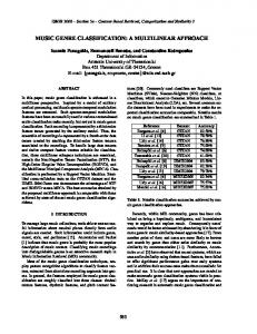
Table 1: frequency bin definition for time-feature extraction Using the DWPT the input music signal can be decomposed into these sub -bands. Each sub -band is then characterized in the time domain by measuring the range of beats that are found. The overall algorithm is show n in figure 1. In order to assure a time -resolution suitable for extracting periodicities in music we have to take into account the properties of the data and of the WPDT. Since the wavelets at any level j are obtained by stretching and dilating the mother wavelet by a factor 2j [2], the time resolution at level j is given by:
Tsec = j
1
⋅ Wsup ⋅ 2 j
S rate
(1)
where Wsup is the wavelet support and j is the decomposition level of the WPDT. The resolution in beat per minute (b.p.m.) at level j is given by:
Fbpm = j
1 Tsec
j
⋅
60 2
(2)
The factor 2 in the above formula has been introduced in order to take into account the sampling theorem. Given music sampled at 44100 Hz, and using the Daubechies4 wavelet (W sup = 8 taps), a maximum resolution of 300 b.p.m., and using equations (1),(2); 9 levels of decomposition are necessary. The time-features are therefore extracted directly from the beat-histogram [10] of the signal. It is calculated adding all the periodicities found in each sub -band to the same graph. The f eatures are: the intensity, the position and the width of the 20 first most intensive peaks. The position of a peak is the frequency of a ‘dominant’ beat,
the intensity refers to the number of times that beat frequency is found in the song, the width corre sponds to the accuracy in the extraction procedure. The peak detection algorithm uses the first derivate of the signal. Additional features used are: the total number of peaks present in the histogram, the histogram max and mean energy and the length in seconds of the song.
Input signal WPDT Sub-band Extraction
WR
WR
WR
AC
AC
AC
PD
PD
PD
Beat-Histogram Time-Feature Encoding Legenda: WR: y[n] = abs(x[n]) AC: autocorrelation function PD: Peak detection
Figure 1: time-feature extraction The idea of the beat -histogram was proposed by G. Tzanetakis et al. [10]. In their work, they demonst rate the usefulness of such a characterization in music classification. The algorithm presented here uses a different analysis methodology (DWPT). Moreover, we take into account a higher number of time -features: 64 time-features and we analyze the input fi le completely by using a different number of decomposition levels. 3.2. Frequency feature The feature set we propose is directly calculated from the frequency spectrum achieved via the DWPT. Given an input signal sampled at 44100 Hz, the DWPT divides the frequency axis between 0 Hz and 44100 Hz in 2j intervals. It is possible to demonstrate that 13 levels of decomposition are necessary in order to have frequency bins matching music notes. With such a resolution, we can propose a new set of frequency featu res that takes into account some characteristics of music. Being able to tell which notes are ‘dominant’ means having a way to
Updated version released Feb. 2003
characterize the music harmony. Moreover, recording the note intensity and position at every octave means estimate implicitly the typology of playing instruments. The spectrum characterization is performed considering frequency intervals matching music octaves (table 2). Frequency Interval 0 HZ (C0) 33 Hz (B0) 33 Hz (C1) 64 Hz (B1) 64 Hz (C2) 128 Hz (B2) 128 Hz (C3) 256 Hz (B3) 256 Hz (C4) 512 Hz (B4) 512 Hz (C5) 1025 Hz (B5) 1025 Hz (C6) 2048 Hz (B6) 2048 Hz (C7) 4096 Hz (B7) 4096 Hz (C8) 8192 Hz (B8) 8192 Hz (C9) 16348 Hz (B9) 16348 Hz (C10) 32769 HZ (>C10)
Bin Numb. 0 1 2 3 4 5 6 7 8 9 10
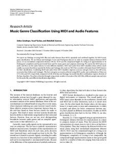
Table 2: frequency bins definition for frequencyfeature extraction For every single frequency bin, we calculate the intensity and position of the first 3 most intensive peaks. Moreover, we consider as a characteristic parameter the total number of peaks in each bin. This value can be interpreted as a measure of the harmonical complexity of the sound we could underestimate. We record the max and mean energy of the spectrum as well: 79 frequency -features in total. Figure 2 shows the algorithm for the frequency -feature extraction process.
Input Signal WPDT Frequency Spectrum Extraction Frequency-Feature Encoding
4.1. k-NN classifier k-NN classifiers are instance -based algorithms taking a conceptually straightforward approach to approximating real or discrete valued target functions. The learning process consists in simply storing the presented data. All instances correspond to points in an n-dimensional space and the nearest neighbors of a given query are defined in terms of the standard Euclidean distance [4]. The probability of a qu ery q belonging to a class c can be calculated as follows:
p (c | q ) =
k ∈K
wk ⋅ 1(kc = c) k∈K
wk
(3)
wk = 1 d (k , q ) where K is the set of nearest neighbors, kc the class of k and d(k,q) the Euclidean distance of k from q. We define K as the set of the first 5 nearest neighbors. 4.2. Ensemble of classifiers An ensemble of classifiers is a set of classifiers whose predictions are combined to classify a query. Typically, the predictions are combined by weighted or unweighted voting. Ensembles of predictors can improve the accuracy of a single classifier, depending on the diversity of the ensemble members [5, 8]. We constructed the ensemble of classifiers using a relatively new approach: pair -wise or round -robin binarization [9]. This methodology converts a c-class problem into a series of two -class problems, using as training set only the appropriate classes and ignoring the others. The query is classified by submitting it to the c(c1)/2 binary predictors. In this work, each ensemble member is a k-NN classifier. The final prediction is achieved by majority voting. The prediction of every single classifier is weighted by its probability (3). 4.3. Feature selection
Figure 2: frequency-feature extraction
4. CLASSIFICATION In order to evaluate the feature -set we use a round -robin ensemble of simple classifiers, i.e. k-NN classifiers. Our dataset consists of 202 songs belonging to 5 different genres. Each song has been labeled manually using [6] as musical-genre reference.
An important issue for k-NN classifiers is that the distance between instances is calculated based on all the attributes. That implies that features meaningful for the classification have the same weight of features less important for that purpose. This fact leads to miss -classification problems and to degradation in the system accuracy. Such a behavior is well known in the li terature and is usually referred to as the curse of dimensionality [4]. We address the problem of high dimensionality (143-dimension feature space) implementing a feature selection strategy based on the concept of information gain [4]. Information gain is an entropy -based measure that
Updated version released Feb. 2003
evaluates the usefulness of a feature with respect to a given set of examples. Using this idea, each feature is ranked with by its discrimination power for the given set of instances. The feature selection is done by selecting only the first N ranked features. In this experiment we changed the number of selected feature from 1 to 25, running the evaluation 25 different times. This kind of feature selection is not meant to be exhaustive. In fact numerous different techniques cou ld have been applied in order to evaluate the feature space: backward hill climbing, forward hill climbing or schemata search. The big draw -back of those techniques is the risk of over-fitting the data. This risk is particularly high in our case, since we deal with a large number of features (143) and relatively few instances. In order to evaluate the accuracy of a round-robin ensemble and a simple k-NN classifier, we performed a stratified 13 fold -cross-validation on the above described dataset.
5. RESULTS Figure 3 shows a comparison between performance of a random classifier, a simple k-NN classifier and the round robin ensemble. In the last two cases, we applied the feature selection procedure described in section 4.3. The round-robin ensemble accura cy has been achieved using the first 17 best ranked features. The k -NN accuracy (63.6%) has been achieved using the full feature set, since the feature selection process didn’t provide a better score. The round -robin ensemble outperforms the random and the simple k-NN classifier achieving a score of 73.3%. Accuracy [%] 80 70 60 50 40 30 20 10 0 Random
simple k-NN
R.R ensemble
Figure 3: classifier accuracy comparison
Table 3 shows the confusion matrix for the round ensemble classification.
-robin
Table 3: genre classification confusion matrix
Q/A C1 C2 C3 C4 C5
C1 29 2 3 1 3
C2 3 21 2 6 4
Legenda: C2 : Rock C4 : Electronic
C3 3 2 32 1 1
C4 1 4 0 31 0
C5 4 10 2 0 30
C1 : Jazz C3 : Classical C5 : Hard Rock
6. CONCLUSIONS This work demonstrates the usefulness of a DWPT applied to signal analysis in the music domain. It shows that new set of music descriptors we propose c aptures some important characteristics of music. The result achieved with a simple k-NN classifier (63.6%) is a good measure of the usefulness of such a characterization. When enhanced to manage multi -class problems (round -robin ensemble), the predictor achieved good results. In fact, the results of our experiment could be even better if we look closely to the classes we chose. Classes C5 (Table 3) is a sub-class of C4 (different styles of the same genre [6]). Merging these classes in one unique “super -class” would increase the total score of our system (80.5%). The basic feature selection strategy we applied assures diversity between ensemble members, leading the ensemble to achieve good classification accuracy. However, as remarked in section 4.3, this kin d of feature selection is not exhaustive and the poor results achieved applying this idea on a simple k-NN confirms this opinion. In a similar evaluation on a problem with 4 classes and 164 instances round -robin classification had an accuracy of 82.1%: ag ain significantly outperforming the simple k NN classifier (71.8%).
Updated version released Feb. 2003
7. REFERENCES [1] Y. Wang, Z. Liu, J.C. Huang, ''Multimedia Content Analysis Using Both Audio and Visual Clues'', IEEE Signal Processing Magazine, 12-36, November 2000. [2] S.G. Mallat, ''A Wavelet Tour of Signal Processing'', Academic Press 1999. [3] C. Hayes, P. Cunningham, P. Clerkin, M. Grimaldi, “Programme-driven music radio”, Proceedings of the 15th European Conference on Artificial Intelligence 2002, Lyons France. ECAI'02, F. van Harmelen (Ed.): IOS Press, Amsterdam, 2002 [4] T. M. Mitchell, ``Machine Learning'', McGraw International Edition, Computer Science Series, 1997
-Hill
[5] T. G. Dietterich, ''Ensemble Methods in Machine Learning'', First International Works hop on Multiple Classifier System, Lecture Notes in Computer Science, J. Kittler & F. Roli (Ed.), 115. New York: Springer Verlag. [6] http://www.allmusic.com. [7] L.K. Hansen, P. Salamon, “Neural Network Ensemble”, IEEE Trans. Pattern Analysis and Machine Learning, vol. 12, 993 1001, 1990. [8] G. Zenobi, P. Cunningham, “Using Diversity in Preparing Ensemble of Classifiers Based on Different Subsets to Minimize Generalization Error”, 12 th European Conference on Ma chine Learning (ECML 2001), L. De Readt & P. Flach (Ed.), LNAI2167, 576-587, Springer Verlag. th [9] J. Fürnkranz, “Round Robin Rule Learning”, Proc. 18 International Conference on Machine Learning (ICML-01), C.E. Brodley & A.P. Danyluk (Ed.), 146 -153, Wil liamstown, MA, 2001.
[10] G. Tzanetakis, G. Essl, P. Cook, ''Automatic Musical Genre Classification of Audio Signals'', In. Proc. Int. Symposium on Music Information Retrieval (ISMIR), Bloomington, Indiana, 2001. [11] J. Pinquier, C. Senac, R. Andre-Obrecht, “Speech and Music Classification in Audio Documents”, ICASSP 2002, Orlando, Florida, May 2002.