Your Place in Space: Classroom Experiment on Spatial Location Theory Margo Bergman, G. Dirk Mateer, Michael Reksulak, Jonathan C. Rork, Rick K. Wilson and David Zirkle Abstract The authors detail an urban economics experiment that is easily run in the classroom. The experiment has a flexible design that allows the instructor to explore how congestion, zoning, public transportation, and taxation levels determine the bid-rent function. Heterogeneous agents in the experiment compete for land use utilizing a simple auction mechanism. Using the data that is collected, a bid-rent function is derived, and the experimental treatment is altered over the course of three sessions to uncover core concepts in urban economics. Moreover, this provides a tangible experience that can be used to help undergraduates relate to urban issues such as the steep rent gradient found around many larger colleges and universities. JEL codes: A22, R1, C9 Keywords: Bid-rent function, classroom experiment, spatial location, urban economics
Acknowledgement Bergman:
[email protected]; Incarnate Word Academy; Mateer: Senior Lecturer, Pennsylvania State University,
[email protected]; Reksulak: Assistant Professor, Georgia Southern University; Rork: Assistant Professor, Georgia State University; Wilson: Professor, Rice University; Zirkle: Instructor, Randolph College. All comments should be directed to Mateer. The work was completed under an NSF Infrastructure grant (SES 00-94800), although that agency bears no responsibility for the contents. Thanks go to the 2004 NSF Workshop on Classroom Experiments in Economics held in Williamsburg, VA. Special thanks go to Lisa Anderson, Catherine Eckel, and Charlie Holt for their help and comments.
1
This classroom experiment is versatile in that it can be applied to many different economic scenarios. In our discussion we focus on an urban application: that of differential locational demand patterns by heterogeneous agents. When teaching urban economics it is sometimes difficult for students to understand spatial location models. Such models are standard for motivating the analysis of urban settings, transportation, and competing taxing authorities. The exercise that follows has three goals. The first is to demonstrate that competitive forces determine the spatial locations of individual citizens and businesses in an urban area. Second, it allows the instructor to demonstrate how other key issues, such as zoning, transportation networks, and differential tax rates, affect the spatial calculus of different actors in the community. Third, students gain firsthand experience at how each of these separate market forces helps to determine where businesses and residences locate. Instructors seeking to motivate how spatial markets work can introduce offcampus apartment rentals surrounding their institution. In many cases, there exists a steep rent gradient within walking distance of the college or university. Introductory courses in economics can benefit from using this exercise to stimulate a more complete comprehension of how agents make optimal decisions given constraints. The exercise presents a public economics application of the Tiebout mechanism (Tiebout 1956). Different treatments can be easily constructed to demonstrate how residents relocate – “vote with their feet” – when municipalities offer more attractive services or comparatively low tax rates.
2
MOTIVATION The bid-rent function is a core concept in urban economic analysis. Its origins can be found in the analysis of land use by the German economist J. H. von Thünen (von Thünen 1826), which relied heavily upon Ricardo’s (1817 [1951]) theory of rent. In his groundbreaking article on the urban land market, Alonso (1964) pointed out that a purchaser acquires two goods (land and location) in one transaction. Therefore, it is possible to trade off a quantity of land against location. The Alonso monocentric model is applicable to economic activities that display a hierarchy of use in terms of distance from the center. The cornerstone of the bid-rent function is the leftover principle, which is the notion that under perfect competition, all nonland profits accrue to the landowner. Because transportation costs associated with undertaking market transactions vary with each location, the amount an economic agent is willing to pay for a particular location will vary negatively with distance, as predicted by Alonso. Each agent has its own bidrent function and competes for land with other agents. The assumption of perfect competition guarantees that agents will bid away their nonland profits at each location, resulting in rents (profits) for the landowner. The use (or activity) that has the highest bid-rent at one point is theoretically the use that will occupy a particular location. In developing a bid-rent function there are three elements that must be determined. First, there is the issue of the rent (profit) that results from some advantage associated with the property. In the case of a business it can be accessibility to suppliers. For residential property it can be distance to the city center or the available amenities. Second, the rent gradient must be determined. Its steepness is determined by the marginal
3
cost of distance for each activity (often embodied as transportation costs) and the friction of space. If there were no frictional issues, each location would be a perfect location. Segregation of land occurs by type, caused by differences in endowments and transportation costs. Third, the combinations of land prices and distances among which the individual (or firm) is indifferent, known as the bid-rent function, is fixed. Households typically have a bid-rent function for urban land that is flatter than the bidrent line for manufacturers so it is not surprising to find households farther from the city center. Creating an individual bid-rent function is relatively straightforward for students. This experiment aids in understanding the dynamic movements of bid-rent functions that occur with changes in endowments, transportation costs, and other economic factors. When combined into a multiple bid-rent function arena, the class experiment demonstrates that segregated land use can quickly result. We often find that students fail to grasp the notion that land use can be segregated, or are unwilling to believe that this could be the case. In most urban settings, the interaction of multiple bid-rent functions is a general equilibrium problem. Many variables are at work and identifying a set of land price/distance locations among which agents are indifferent requires students to think simultaneously on many different levels. The advantage of this classroom experiment is that one factor can be isolated and students can observe how this affects the bid-rent function.
4
INSTRUCTOR PROCEDURES The exercise can be run with any size class in approximately 30 minutes. It is designed to be run with small classes (n < 30), although with large classes it would be possible to partition the class into groups of 30 or less and run the exercise simultaneously in each group. The goals of the class experiment are to introduce students to spatial location models, to get students to think about tradeoffs between price and relative cost and to illustrate that segregation of land use occurs by type, because of differences in endowments and transportation costs. The exercise proceeds through three distinct treatments, with each treatment taking approximately 10 minutes to complete. The entire exercise can be carried out by a single person although it is helpful to have a second person record the data into a spreadsheet so that the results are available for analysis upon completion of the exercise.
Materials In order to conduct this experiment you will need: •
Decks of cards (ace through 10), greater than or equal to the numbers of students in the class.
•
Red and black poker chips (or some other, easily distributed and hidden marker) in equal numbers, enough for everyone in the class to receive one chip.
•
Opaque container.
•
A payoff sheet for each student (there are two types of payoff sheets).
•
A recording sheet.
•
An instruction sheet.
Copies of the various instruction and payoff sheets are provided in the Appendix. 5
Pre-Experiment Preparations All of the preparations can be handled beforehand. All that is needed is: •
A spreadsheet or some other device to generate bid-rent functions.
•
Oral instructions to be read by the experimenter (see the Appendix).
•
An overhead projector for the student instructions or enough individual sheets with the printed student instructions (see the Appendix).
•
Copies of the student record sheets.
•
A spreadsheet or other method to store the data generated.
Experiment Instructions The following steps are taken to run the experiment. Throughout, we assume that an overhead projector is used, but similar sequences can be used for materials that are passed out by hand. 1. A short set of instructions are read (see the Experimenter’s Instructions in the Appendix). These provide minimal information to the students but give them an overview to the experiment. Students should be told enough information so that they can participate in an informed manner without giving them all the details. 2. The chips should be placed in an opaque container, and students should take them one at a time. Students who receive a RED chip are in Group A; students receiving a BLACK chip are in group B. The chips are to be kept hidden from other students, so that the exact number of each type is not obvious. Chips are used in order to reduce possible confusion between the “type” card, which tells the student which type they are, and the “unit” card which is the card they are
6
purchasing. As they draw a chip, distribute the appropriate subject instructions to each person. 3. Give each student a couple of minutes to review the subject instruction sheet and work through the example so that they know how to calculate their profits. If, in period 1, a subject purchases a card with a value of 4 for a price of 20, then their record sheet would look like that given in Table 1. Total costs are calculated by multiplying the value on the card bought, 4, by the cost per unit, 20. Add to this the price of the card, 20, to get a total cost of 100. Subtract 100 from their endowment of 120, and the result is earnings of 20. [Table 1 about here]
4. Once everyone understands the process, there are three primary points that need to be repeated: The first is that everyone can only buy once in each period. The second is that participants should attempt to generate the largest rent possible. If you do not bid during a period then your earnings for that period are zero. Third, participants who over-bid lose the amount that they overbid in that round from their total profits. These simple rules are designed to keep the experiment flowing and to minimize distractions. In order to maintain interest, incentives should be used. Something as simple as distributing candy for students with the highest profit at the end of the class is an option if there does not already exist a monetary or grade-based incentive structure. 5. The experiment begins by showing students the reduced deck of cards that ranges from ace through 10. Re-iterate to the students that a limited number of draws
7
will be made from this stack. Each card represents a commodity and they will bid on these one at a time. To get students to participate, randomly select one student to draw from the deck. The total number of cards chosen in each period should be large enough to engage interest, but not so large that it takes too much time to get through each session. Having 20-30 percent of the total number of cards become available in each round is sufficient. In a class of 30, this would be between 6 and 9 cards. 6. Participants are now asked to bid. Participants are reminded that they can only bid once in each period. An ascending oral (English) auction is then used to solicit bids. The auctioneer begins and bids are accepted for each card. Once all the cards are exhausted in that period the results from that round are recorded and the next period begins. The auctioneer should move the exercise along quickly and force students to make fast decisions. 7. All bids and winnings are recorded. 8. Treatment 2 begins. In treatment 2, a fee is placed on purchases made by type B subjects. The endowments and costs per unit for all subjects remain the same for both type A and type B. Each subject retains their original type and instruction sheet. This new fee is already written into the record sheet for all type B’s. Briefly go over the changes so that everyone understands that the financial calculus is different. Repeat steps 4, 5, 6, and 7. Table 2 provides an example of the earnings record sheet with the new fee. Given the example from the instructions for treatment 1, a subject who purchased a 4 card for a price of 20, would now have a total cost of 120, resulting in earnings of 0.
8
[Table 2 about here]
9. Treatment 3 begins. In treatment 3, the cost per unit for type A’s is lowered. The endowments and costs per unit for all subjects remain the same for type B. The extra fee from treatment B is removed. The type B’s return to their original costs. This is indicated on their information sheet. Each subject retains their original type and instruction sheet. This new per unit cost is already written into the record sheet for all type A’s. Briefly go over the changes so that everyone understands that the financial calculus is different. Repeat steps 4, 5, 6, and 7. 10. After treatment 3 ends the students should tally their winnings. What to Expect The bid-rent functions for each treatment are generated from the endowment and per unit transportation cost (fixed cost). There are two types of consumers, type A with a smaller endowment, but a lower per unit transportation fixed cost, and type B, with a larger endowment, and a higher per unit transportation fixed cost. In order to generate the basic equilibrium bid-rent function, use the following formula: (1)
BRi = Ei − ti D ,
where BRi is the bid-rent function for either type A or type B. Ei is the endowment for that type, ti is each type’s fixed per unit transportation cost and D is the distance from the city center. The bid-rent functions of the various treatments can be found by altering either the transportation cost, as in the example treatment 3, or by adding a tax or subsidy, as in treatment 2, which is effectively a reduction or increase in the endowment, respectively.
9
Once both bid-rent functions are generated, they can be plotted on the same graph in order to generate the intersection point. The theory states that, all else equal, the type with a higher transportation cost should locate to the left of the intersection, and the other type will locate to the right. Table 3 provides an example. [Table 3 about here] Given two types, Group B with an endowment of 120 and transportation cost of 20, and Group A with an endowment of 80 and a transportation cost of 10, the following bid rent functions are generated in Figure 1. The point of intersection is 4, indicating that the A’s should locate from 5 to 8, and the B’s should locate from 1 to 3, and both are indifferent at 4. [Figure 1 about here]
On the data record sheet the student should record the type of the buyer of a card, the number of the card that they bought, the price they paid, and the maximum price they should have paid, based on their endowment and transportation cost. In order to compare the experimental data to the theoretical outcome, plot the price paid vs. the two maximum prices at each location. It should show that the buyers to the left of the intersection point are the type with a higher transportation cost.
RESULTS To motivate a robust class discussion it is easy to generate real-time data from the experiment you have just completed. This provides a platform for a discussion of spatial location models. The students should now understand that changes in endowments and
10
costs will affect where agents locate. As part of the lesson it is straightforward to explain how the bid-rent functions were created and illustrate the corresponding bids from the exercise. Below we include the results from experiments run during the 2005-2006 academic year. The experiments were conducted with both Principles and Intermediate Microeconomics students at two universities: Georgia Southern University and Pennsylvania State University. Figure 2 plots the prices paid under the no fee treatment, while the two lines indicate the bid-rent function for each type at that location. There were 126 data points in each treatment (18 points in each of 7 sessions). On visual inspection, the subjects in the first treatment often overpaid for the cards that they were purchasing, because many of the data points are above and to the right of the Nash equilibrium lines. In our experience, students initially get caught up in the rush of participating in the auction, leading them to overbid without properly calculating and/or forgetting what their bid should be. As the auction progresses, students relax and perform closer to theoretical predictions.1 Note that as the theory predicts, there were 3 cards not purchased at values 8, 9 and 10. [Figure 2 about here]
In the second treatment, the type B’s paid an additional fee. Theoretically, this shifts the intersection point to the left compared with the data from treatment 1 plotted on Figure 2.
1
Overbidding often happens in the beginning, as students acquaint themselves with the experiment. As our results demonstrate, students approach the theoretical outcomes as their experience in the experiment increases. Such an occurrence opens the door for the instructor to have a discussion about the importance of rationality of agents for the predictions of not only this particular model, but also many other economic models that we teach.
11
From the data plotted on Figure 3, subjects shift in their price and outcomes converge to the Nash equilibrium. There were 5 cards that were not purchased as predicted by the theory; again at values 8, 9, and 10. [Figure 3 about here]
In the third treatment, the per unit cost for type A’s is lowered and this rotates the type A bid-rent function outward. Compared with treatment 1 this shifts the intersection point to the left and affects the point at which the type A curve intersects the location axis. In this case, it shifts it far enough that all of the locations can be purchased by both types of players. Figure 4 shows that subjects cluster around the Nash Equilibrium, often choosing to underpay rather than bid over the optimal purchase price. [Figure 4 about here]
CLASS DISCUSSION AND EXTENSIONS From this experiment students should be able to see that in a spatial setting land use will be segregated by type. This segregation is a result of two factors: endowments and transportation costs. Finally, this exercise can demonstrate how to take a multivariate function and simplify it into a two-dimensional graph. One goal for this classroom experiment is to get students to appreciate how changes in one of the factors alter the bid-rent function. The fee in treatment 2 has the effect of lowering the endowment of type B’s, but has no impact on the transportation costs type B’s face. Consequently, the bid-rent function undergoes a parallel shift, as the agent is now able to afford less at all locations. This helps students to see that endowment changes cause shifts in the bid-rent function.
12
Treatment 3 is designed to show that changes in transportation costs cause a rotation in the bid-rent function. An important concept to emphasize is that changes in transportation costs only affect type A’s if they locate outside the city center. Because no transportation costs are incurred in the city center, there is no change in what type A’s are willing to bid for that location. Thus, lowering the transportation cost of type A’s resulted in an outward rotation in the bid-rent function. Treatments 2 and 3 also demonstrate to students how changes in one bid-rent function affect the land available to both types. By imposing a tax on type B’s, type A’s were able to expand the land available to them at the expense of type B. By lowering the transportation costs of type A’s, they were able to buy land that was previously too far away. But at the same time, the transportation savings allowed type A’s to bid more competitively against the B’s, resulting in a smaller range of B-exclusive land. Once students learn the basic mechanics of the bid-rent function, there are many related discussions that can take place. For example, it is useful to have students think of type A’s as residents and type B’s as firms. Students can discuss why firms would have higher transportation costs than individuals. Do they normally see firms in the city center? Is this why? This gives a nice segue for discussing the notion of a monocentric city and the creation of central business districts and residential pockets. In the same vein, one can ask what would happen if public transportation were expanded? Students could respond that this would lower resident’s transportation costs, resulting in an outwards rotation of the bid-rent function and an expansion of the area where people are willing to live. This can lead to a discussion about the expansion of the suburbs and the willingness of individuals to increase commuting time.
13
This in turn can be linked to what happens when congestion results from too many people moving into the suburbs. Can this cause people to move back towards the center? What effect would they have on land patterns? Are people willing to pay more for land inside the tolls? Even tangential questions about the efficacy of tolls on congestion could be discussed. Another extension is to bring in the notion of zoning. Suppose in treatment 3 an urban growth boundary was placed at position 7. What effect does this have? Students will see that no one will locate beyond 7, but there will be no effect on the price of land within the boundary, as the leftover principle has already bid the price up to its maximum. Alternatively, one could impose a simple form of nuisance zoning in Treatment 1 by banning B’s from buying locations 2 and 3. Students should recognize that there would be a discontinuity in overall pricing, as only A’s would bid for these positions. However, B’s would be the exclusive purchasers of positions 1 and 4. Moreover, we now have a distribution of land in which there are two pockets of B’s and two pockets of A’s. Once students see that land segregation can occur in pockets, as opposed to just two broad areas, a discussion about multicentric models (Ogawa and Fujita 1980; Bogart 1998) can be initiated. Students may be asked if there are any other rationales for why type B’s may not bid for particular areas, leading to conversations about interstates, airports and the general importance of transportation systems. The value of the bid-rent function is that once understood, it allows for numerous policy discussions. Most importantly, the policy issues are often interrelated, so that discussions of the growth of the suburbs, congestion, and transportation can all be
14
brought together in one setting. Such policy linkages allow students to think outside the box and see how one policy cannot be viewed in isolation. Confronting and appreciating these general equilibrium effects in action is particularly enlightening for students.
CONCLUSION This experiment demonstrates how competitive forces drive the spatial locations of individual citizens and businesses in an urban setting. Moreover, it provides a platform that the instructor can use to extend the understanding of spatial location theory and the location of rents in a monocentric model. The treatments described are designed to enhance student understanding of the factors that influence locational decisions. The simplicity of the bid-rent function and the monocentric city model is that it opens itself for discussion in various aspects of public policy. Although the primary focus for such a model is in an urban economics class, the fact that this experiment is self-contained means that is well-suited for use in courses on urban and public policy that have little or no formal economic components to them.
15
REFERENCES Alonso, W. 1964. Location and land use: Toward a general theory of land rents. Joint Center for Urban Studies Publication Series. Cambridge, Mass: Harvard University Press. Bogart, W. 1998. The economics of cities and suburbs. Upper Saddle River, NJ: Prentice Hall. Ogawa, M. and M. Fujita. 1980. Equilibrium land use patterns in a nonmonocentric city. Journal of Regional Science 20(4):455–75. Ricardo, D. 1817 [1951]. On the principles of political economy and taxation. vol. 1 of The collected works of David Ricardo, ed. P. Sraffa and M. Dobb. Cambridge: Cambridge University Press. von Thünen, J. H. 1826. Der isolierte Staat in Beziehung auf Landwirtschaft und Nationalölkonomie, oder Untersuchungen über den Einfluß, den die Getreidepreise, der Reichtum des Bodens und die Abgaben auf den Ackerbau ausüben, Vol. I (1826); Vol. II.i (1850), Vol. II.ii and Vol. III (1863); in English translation as The isolated state, ed. P. Hall (Oxford, 1966). Tiebout, C. M. 1956. A pure theory of local expenditures. Journal of Political Economy 64(5): 416–24.
16
APPENDIX Experimenter Instructions In this experiment you will be purchasing cards. You will always be a buyer. You are not buying the cards from me, I am the auctioneer. You need to pay careful attention to what is happening in the experiment. You are trying to maximize the difference between how much you pay for a card, the additional cost per unit of that card, and the endowment that you have. Each card is numbered A (which is a 1) through 10. The number on the card represents how many “units” that card contains. You are required to pay an additional amount per unit, on top of what you pay for the card itself. There are ___ number of cards total, but only ___ of them become available in each period. (Replace “blanks” with numbers.) You purchase these cards in an oral auction, where the highest bidder wins that card. I will be coming around, and you will pick a checker out of this container. Half the checkers are black, and half are red. Following this I will pass out the record sheets for the experiment. Please keep the color of your checker confidential. You have received your record sheet. Please keep your record sheet confidential throughout the experiment. The experiment will be conducted as follows: A card will be drawn from the deck of randomly shuffled cards here. This is one of the ___ number of cards that will become available for purchase in that period. The auctioneer will announce the value of the card, and that bidding is open at a certain value. If you wish to buy the card, raise your hand, and when called on, announce your bid. This will continue until no more people wish to bid, and the auctioneer will announce that bidding is over. Whoever wins the card will write down on their record sheet the unit value of the card, and the amount they paid. Once you buy a card in a particular period you cannot buy another. If you do, you will be disqualified from the rest of the experiment. 17
This will continue for all the cards that will be sold in a particular round. You calculate your earnings by taking the amount you have, minus the price you paid, minus the value of the card you purchased times the price per unit listed on your record sheet. If there is an additional fee listed, you must add this to your purchase price when you calculate your earnings. Make sure you are putting this information under the section entitled Session 1. Does anyone have any questions? Once the experiment is done, you will hand in your completed Record Sheet. Additional rules and examples are on the Subject Instruction handout. Now we will begin the second session. The mechanism will be the same, but you should refer to your information sheet to determine if your endowment or price per unit has changed, or if there is an additional fee. If there is an additional fee, you must add this to your purchase price when you calculate your earnings. Make sure you are recording information under the section entitled Session 2.
Now we will begin the third session. The mechanism will be the same, but you should refer to your information sheet to determine if your endowment or price per unit has changed, or if there is an additional fee. If there is an additional fee, you must add this to your purchase price when you calculate your earnings. Make sure you are recording information under the section entitled Session 3.
18
Subject Instructions/Payoff Sheets.
You are in Group A
This is an experiment in economic decision-making. You are going to be asked to make choices. Your choices will determine your pay-offs in this game. There are two groups of buyers in this game; those in Group A and those in Group B. Your Endowment and Cost are unique to your group. Your Endowment is: Your cost per unit is:
80 10
Payoffs The Auctioneer has a stack of 20 cards, including “Ace, 2, 3, 4, 5, 6, 7, 8, 9, 10” (“Ace” has a value of one.) Six cards will be randomly selected in each period. In each period, you will be allowed to bid for cards. There are two possible outcomes. I)
You do not buy a card in a period. Your endowment disappears and your earnings are zero. You buy a card. Your earnings are calculated as shown below.
II)
Note: YOU MAY ONLY BUY ONE CARD IN EACH PERIOD.
Example Suppose you buy a card with the card value “6” at a price of 10. Then your earnings will be calculated by: Endowment – Auction Price – (Card Value x Cost per Unit). Practice this below (fill in the values): Period
Endowment
Card Bought
1
80
6
Auction Price 10
Cost per Unit 10
The correct solution is: 80 – 10 – (6 x 10) = 80 – 10 – 60 = 10
19
Total Cost
Earnings
Earnings Record Sheet – Group A Your Name:
Session 1 Period
Endowment
1 2 3
80 80 80
Card Bought
Auction Price
Cost per Unit
Total Cost
Earnings
Total Cost
Earnings
Total Cost
Earnings
10 10 10
Session 2 Period
Endowment
1 2 3
80 80 80
Card Bought
Auction Price
Cost per Unit
10 10 10
Session 3 Period
Endowment
1 2 3
80 80 80
Card Bought
Auction Price
Cost per Unit
5 5 5
Note: If you do not purchase a card, then your earnings for that period are automatically $0.
20
You are in Group B
This is an experiment in economic decision-making. You are going to be asked to make choices. Your choices will determine your pay-offs in this game. There are two groups of buyers in this game; those in Group A and those in Group B. Your Endowment and Cost are unique to your group. Your Endowment is: Your cost per unit is:
120 20
Payoffs The Auctioneer has a stack of 20 cards, including “Ace, 2, 3, 4, 5, 6, 7, 8, 9, 10” (“Ace” has a value of one.) Six cards will be randomly selected in each period. In each period, you will be allowed to bid for cards. There are two possible outcomes. III)
You do not buy a card in a period. Your endowment disappears and your earnings are zero. You buy a card. Your earnings are calculated as shown below.
IV)
Note: YOU MAY ONLY BUY ONE CARD IN EACH PERIOD.
Example Suppose you buy a card with the card value “3” at a price of 40. Then your earnings will be calculated by: Endowment – Auction Price – (Card Value x Cost per Unit). Practice this below (fill in the values): Period
Endowment
Card Bought
1
120
3
Auction Price 40
Cost Per Unit
Total Cost
20
The correct solution is: 120 – 40 – (3 x 20) = 120 – 40 – 60 = 20
21
Earnings
Earnings Record Sheet – Group B Your Name:
Session 1 Period
Endowment
1 2 3
120 120 120
Card Bought
Auction Price
Cost per Unit
Total Cost
Earnings
Cost per Unit
Extra B-fee
Total Cost
20 20 20
20 20 20
Cost per Unit
Total Cost
20 20 20
Session 2 Period
Endowment
1 2 3
120 120 120
Card Bought
Auction Price
Earnings
Session 3 Period
Endowment
1 2 3
120 120 120
Card Bought
Auction Price
Earnings
20 20 20
Note: If you do not purchase a card, then your earnings for that period are automatically $0.
22
Sample Treatment 1 140 120 Price
100 80 60 40 20 0 0
1
2
3
4
5
6
7
8
9
Location Group B
Group A
FIGURE 1. Plot of the bid-rent functions for two groups.
23
10
Treatment 1 - All Sessions 160 140 120 100 Price
80 60 40 20 0 0
2
4
6
8
10
Card Value
A
B
A Nash
B Nash
FIGURE 2. Experimental outcomes under the no fee (baseline) treatment.
24
No Bids
Treatment 2 - All Sessions
120 100
Price
80 60 40 20 0 0
2
4
6
8
10
12
Card Value
A
B
A Nash
B Nash
FIGURE 3. Experimental outcomes under the treatment with a fee.
25
No Bids
Treatment 3 - All Sessions 140 120 100
Price
80 60 40 20 0 0
5
10
15
Card Value
A
B
A Nash
B Nash
FIGURE 4. Experimental outcomes under a lower per unit price for group A.
26
20
Table 1. Sample Record Sheet for Group B Subjects.
Period 1 2 3
Endowment 120 120 120
Card Bought 4
Auction Price 20
27
Cost Total per Unit Cost 20 100 20 20
Earnings 20
Table 2. Sample Earnings Sheet for Group B Subjects with a Fee.
Period 1 2 3
Endowment 120 120 120
Card Bought 4
Auction Price 20
28
Cost per Unit 20 20 20
Extra B-fee 20 20 20
Total Cost 120
Earnings 0
Table 3. Sample endowments and transportation costs for two groups.
Endowment
Transportation Cost
Group A
120
20
Group B
80
10
29