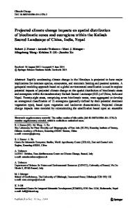
Climate change impacts on hydrological science

Climate change impacts on hydrological science How the climate change agenda has lowered the scientific level of hydrology Demetris Koutsoyiannis Department of Water Resources and Environmental Engineering School of Civil Engineering National Technical University of Athens, Greece ([email protected], http://itia.ntua.gr/dk/) Presentation available online: http://itia.ntua.gr/1847/

Prologue: setting the scene Παρρησίᾳ γὰρ ἔγωγε χρώμενος φυσιολογῶν χρησμωδεῖν τὰ συμφέροντα πᾶσιν ἀνθρώποις μᾶλλον ἂν βουλοίμιν, κἄν μηδεὶς μέλλῃ συνήσειν, ἤ συγκατατιθέμενος ταῖς δόξαις καρποῦσθαι τὸν πυκνὸν παραπίπτοντα παρὰ τὸν πολλῶν ἔπαινον. As I study nature, I would prefer to speak bravely about what is beneficial to all people, even though it be understood by none, rather than to conform to popular opinion and thus gain the constant praise of the many. (Epicurus, Vatican Sayings, 29) http://sqapo.com/epicurus.htm

Epicurus 341–270 BC

Bring’ vor, was wahr ist; Schreib' so, dass es klar ist Und verficht's, bis es dir gar ist!

DK’s variant: “what is true” → what I believe is true

Put forward what is true; So write that it may be clear Fight for it to the end!

(Ludwig Boltzmann, Vorlesungen über die Principe der Mechanik, 1897)

http://en.wikipedia.org/wiki/Ludwig_Boltzmann

Ludwig Boltzmann 1844 – 1906

D. Koutsoyiannis, Climate change impacts on hydrological science

2

Part 1 Some (soft*) facts about recent climate with particular emphasis on processes relevant to hydrology *results

from analyses of complex data sets or from other studies

Ocean heat content has been increased 0.095 Annual or 3-monthly

0.076

10-year climate (average of past 10 years)

150

0.057

100

50 0

0.019 0

-0.019

-50 -100 1950

0.038

Equivalent temperature, K

200

253 ZJ → 0.096 K

Upper ocean (0-2000 m) heat content, ZJ

250

-0.038 1960

1970

1980

1990

2000

2010

2020

• Data: NODC upper ocean (0-2000 m) heat content

(from https://www.nodc.noaa.gov/OC5/3M_HEAT_CONTENT/basin_data.html; conversion into equivalent temperature using data from http://climexp.knmi.nl/selectindex.cgi resulting in a conversion factor of 2640 ZJ/K, somewhat lower than in Koutsoyiannis, 2017).

• Result: During the 50-year period 1968 -2018 there has been an increase of 253 ZJ in the upper ocean heat content averaged globally at a 10-year climatic scale; this corresponds to a temperature increase of 0.096 K (average rate 0.018 K/decade). D. Koutsoyiannis, Climate change impacts on hydrological science

4

Temperature of the lower troposphere has been increased

265

0.35 K

Lower tropospheric temperature, K

266

264

263 Monthly

10-year climate (average of past 10 years) 262 1970

1980

1990

2000

2010

Updated with data of June 2018

2020

• Data: UAH satellite data for the lower troposphere (global average) gathered by advanced microwave sounding units on NOAA and NASA satellites

(from http://www.nsstc.uah.edu/data/msu/v6.0/tlt/uahncdc_lt_6.0.txt with monthly averages from http://www.drroyspencer.com/2016/03/uah-v6-lt-global-temperatures-with-annual-cycle/).

• Result: During the 30-year period 1988 – 2018 there has been an increase of 0.35 K in the globally averaged 10-year climatic temperature (increase 0.11 K/decade). D. Koutsoyiannis, Climate change impacts on hydrological science

5

Earth surface temperature has been increased 100

296

From monthly time series

294

From annual time series 10

288 286 284

Variance, K²

290

0.75 K

Temperature, K

292

1

0.1

282 280

Monthly

12-month moving average

10-year climate

0.01

2020

2012

2004

1996

1988

1980

1972

1964

1956

1948

278

0.1

1 Time scale, years

10

• Data: Monthly NCEP/NCAR R1 2m air temperature (K) averaged over the globe (from NCEP-NCAR Reanalysis 1, retrieved through KNMI Climate Explorer, http://climexp.knmi.nl/data/inlhtfl_0-360E_-90-90N_n.dat) • Result 1: During the 60-year period 1958 – 2018 there has been an increase of 0.75 K in the globally averaged 10-year climatic temperature (increase 0.13 K/decade). • Result 2: The climatic temperature has been fluctuating, slightly dropping before 1978 and then increasing. The fluctuation is consistent with the Hurst-Kolmogorov dynamics (long-term changes) with a high Hurst parameter, H = 0.93. D. Koutsoyiannis, Climate change impacts on hydrological science

6

A real-world process as seen in the longest instrumental record

Minimum water depth (m)

Hurst-Kolmogorov dynamics—Or: Earth’s perpetual change 7

Nile River annual minimum water level (849 values)

Annual

6

30-year average

5 4

3 2 1 0 600

700

800

900

1000

1100

1200

1300

1400

1500

A “roulette” process

Minimum roulette wheel outcome

Year AD 7

"Annual"

6

30-"year" average

Each value is the minimum of m=36 roulette wheel outcomes. The value of m was chosen so that the standard deviation be equal to the Nilometer series

5 4

3 2 1 0 600

700

800

900

1000

1100

1200

1300

1400

1500

"Year"

Nilometer data: Koutsoyiannis (2013) D. Koutsoyiannis, Climate change impacts on hydrological science

7

The climacogram: A simple statistical tool to quantify change across time scales • Take the Nilometer time series, x1, x2, ..., x849, and calculate the sample estimate of variance γ(1), where the superscript (1) indicates time scale (1 year)

• Form a time series at time scale 2 (years): x(2)1 := (x1 + x2)/2, x(2)2 := (x3 + x4)/2, ..., x(2)424 := (x847 + x848)/2 and calculate the sample estimate of the variance γ(2). • Repeat the same procedure and form a time series at time scale 3, 4, … (years), up to scale 84 (1/10 of the record length) and calculate the variances γ(3), γ(4),… γ(84).

• The climacogram is a logarithmic plot of the variance γ (κ) (or alternatively the standard deviation σ(κ)) vs. scale κ. • If the time series xi represented a pure random process, the climacogram would be a straight line with slope –1 (the proof is very easy).

• In real world processes, the slope is different from –1, designated as 2H – 2, where H is the so-called Hurst coefficient (0 < H < 1). • The scaling law γ(κ) = γ(1) / κ2 – 2H defines the Hurst-Kolmogorov (HK) process. • High values of H (> 0.5) indicate enhanced change at large scales, else known as long-term persistence, or strong clustering (grouping) of similar values. D. Koutsoyiannis, Climate change impacts on hydrological science

8

7

30-year average

5 4

3

• The Hurst-Kolmogorov process seems consistent with reality.

2

• The Hurst coefficient is H = 0.87 (Similar H values are estimated from the simultaneous record of maximum water levels and from the modern, 131-year, flow record of the Nile flows at Aswan).

0

• The Hurst-Kolmogorov behaviour, seen in the climacogram, indicates that (a) long-term changes are more frequent and intense than commonly perceived, and (b) future states are much more uncertain and unpredictable on long time horizons than implied by pure randomness.

Annual

6

1

600

700

800

Bias

Minimum water depth (m)

The climacogram of the Nilometer time series

Variance (m²)

1

900

1000

1100

1200

1300

1400

1500

Year AD

The classical statistical estimator of standard deviation was used, which however is biased for HK processes

0.1

Empirical (from data) Purely random (H = 0.5) Markov Hurst-Kolmogorov, theoretical (H = 0.87) Hurst-Kolmogorov adapted for bias

0.01 1

10

100 Scale (years)


9

Latent heat net flux is fluctuating 95

10 Monthly



90

Variance, (W/m²)²

Latent heat flux, W/m²

From annual time series

85

80

1 2020

2012

2004

1996

1988

1980

1972

1964

1956

1948

75

0.1

1

10

Time scale, years

• Data: Monthly mean of latent heat net flux averaged over the globe (from NCEP-NCAR Reanalysis 1, retrieved through KNMI Climate Explorer, http://climexp.knmi.nl/data/inlhtfl_0-360E_-90-90N_n.dat Monthly). • Result: The latent heat net flux has been fluctuating and nothing unprecedented is currently experienced. The fluctuation is consistent with the Hurst-Kolmogorov dynamics with a high Hurst parameter, H = 0.93.


10

Land albedo is (slightly) fluctuating 0.40

Land albedo

0.38

0.36

0.34

0.32

0.30 2000

Monthly 2005

12-month moving average 2010

2015

2020

• Data: Monthly albedo averaged over land (from Clouds and the Earth's Radiant Energy System—CERES, subset over land and kindly provided by Willis Eschenbach). • Result: The land albedo has been fluctuating showing a downward trend in the 21st century, which is consistent with the upward trend of temperature. The data availability is too short to make any conclusions about the long-term behaviour. D. Koutsoyiannis, Climate change impacts on hydrological science

11

Precipitable water is fluctuating 34

Monthly

100




Variance, mm²

30 28 26 24

1

0.1

22 20

0.01

2020

2012

2004

1996

1988

1980

1972

1964

1956

18

1948

Totlal precipitable water, mm

32

0.1

1 Time scale, years

10

• Data: NCEP/NCAR R1 precipitable water averaged over the globe (from NCEP-NCAR Reanalysis 1, retrieved from NOAA, http://www.esrl.noaa.gov/psd/cgi-bin/data/testdap/timeseries.pl). • Result: The precipitable water over the globe has been fluctuating with lowest values during the 1980s and highest values during the 1950s and 2010s. The fluctuation is consistent with the Hurst-Kolmogorov dynamics with a high Hurst parameter, H = 0.92. D. Koutsoyiannis, Climate change impacts on hydrological science

12

Precipitation is fluctuating 130

Monthly

1000



120


100

Variance, mm²

Precipitation, mm

110

90 80

10

70 60 1

2020

2012

2004

1996

1988

1980

1972

1964

1956

1948

50

0.1

1 Time scale, years

10

• Data: NCEP/NCAR R1 precipitation averaged over the globe (from NCEP-NCAR Reanalysis 1, retrieved from NOAA, http://www.esrl.noaa.gov/psd/cgi-bin/data/testdap/timeseries.pl). • Result: Precipitation has been fluctuating and nothing unprecedented is currently experienced at the global scale. Lowest values have occurred during the 1980s and highest values during the 1960s and 2010s. The fluctuation is consistent with the Hurst-Kolmogorov dynamics with a high Hurst parameter, H = 0.94. D. Koutsoyiannis, Climate change impacts on hydrological science

13

Global river flow is fluctuating Variance

0.001

Empirical HK adapted for bias

0.0001 1

10

Time scale (years)

10-year moving average

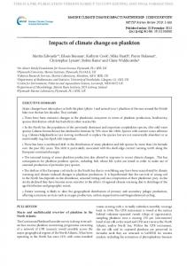
• Source of graph: Dai (2016); the red line (10-year climate) and the climacogram on the right have been produced after digitizing the original graph on the left. • Result 1: River flow has been fluctuating and nothing unprecedented is currently experienced at the global scale. The fluctuation is consistent with the HurstKolmogorov dynamics with a Hurst parameter H = 0.75. • Result 2: River flow fluctuation is in phase with precipitation fluctuation; note though that the precipitation time series has large differences from that of the previous slide. D. Koutsoyiannis, Climate change impacts on hydrological science

14

River flow trends are alternating Total

Stations with trends Positive Negative #stations #stations % #stations % North America South America

Slopes of trends Positive Negative hm3/year hm3/year

190

7

3.7

12

6.3

5.6

-10.7

206

12

5.8

2

1.0

5.3

-19.6

Europe

186

6

3.2

6

3.2

2.0

-0.6

Asia

167

7

4.2

21

12.6

24.5

-8.9

Africa

83

0

0.0

18

21.7

-

-7.6

Oceania

84

2

2.4

16

19.0

2.1

-3.2

916

34

3.7

75

8.2

9.1

-7.2

Total

• Source of table: Su et al. (2018); among results for different assumptions contained in the paper, those taking account of long-term persistence are reproduced here. • Result: River flow at world’s largest rivers show some positive and negative trends. Negative trends are more common than positive in number, but have slightly lower slopes, so that eventually overall the positive slopes surpass the negative ones (9.1 vs -7.2 hm3/year). D. Koutsoyiannis, Climate change impacts on hydrological science

15

Record rainfall is not increasing Q, R

E

K, L, M, W

1 (A)

1860

2 (B-C)

1880

2 (D-E)

1900

1920

3 (F-H)

1940

3 (I-K)

9 (L-T)

1960

2 (U-V)

1980

1 (W)

2000

2020

• Data: World record point precipitation measurements compiled in Koutsoyiannis and Papalexiou (2017) for various time scales (durations) ranging from 1 min to 2 years; locations and time stamps of the events producing record rainfall are shown. • Fact: Highest frequency of record rainfall events occurred in the period 1960-80; later the frequency was decreased substantially. D. Koutsoyiannis, Climate change impacts on hydrological science

16

Annual maximum rainfall has been (slightly) increased in some areas

Dry

Wet • Source of graphs: Donat et al. (2016); Rx1day denotes the annual-maximum daily precipitation • Result: The climatic value of annual maximum daily rainfall of the 30-year period 1980 – 2010, compared to that of 1960-80, is greater by 5% for dry areas and by 2% for wet areas. D. Koutsoyiannis, Climate change impacts on hydrological science

17

Increasing trends on annual maximum daily rainfall have been more frequent than decreasing ones

• Source of graphs: Westra et al. (2013); 8326 stations with more than 30 years of data over the period from 1900 to 2009 (the average record length is 53 years). • Result: Using the Mann-Kendall test, 8.5% were found with positive trends and 2% with negative, against an expected (for the specific test) 2.5% for each direction. • Note: The test was done assuming independence while an assumption of HK dependence would give lower percentages (perhaps adding to 5%). D. Koutsoyiannis, Climate change impacts on hydrological science

18

Data on “rainfall intensification” (sic) do not show unprecedented conditions of rainfall regime Source of graph: Panthou et al. (2018), entitled “Rainfall intensification in tropical semi-arid regions: the Sahelian case”

Note: “hydroclimatic intensity” (panel d) is defined here as mean intensity of rainy days divided by number of rainy days (mm d-2 !)

From abstract: “The analysis of the daily data leads to the assertion that a hydroclimatic intensification is actually taking place in the Sahel, with an increasing mean intensity of rainy days associated with a higher frequency of heavy rainfall.” Question: Is it intensification or fluctuation? D. Koutsoyiannis, Climate change impacts on hydrological science

19

Flood occurrences have been fluctuating through the centuries (1)

• Source of graph: Caporali et al. (2005): Number of flood events, distributed by intensity, of the Arno River, which caused damage in Florence between the 12th and 20th centuries. • Result 1: There is prominent fluctuation with fewer floods in the 20th century than in most other centuries. • Result 2: Fewer high- and medium-intensity floods occured in the 20th century than in all but one other centuries. D. Koutsoyiannis, Climate change impacts on hydrological science

20

Flood occurrences have been fluctuating through the centuries (2)

Number of floods per decade

Atlantic basin

Mediterranean basin

• Source of graph: Barriendos et al. (2006): Flood frequency, estimated from documents and archives in Spain for the last millennium. • Result: Number of floods fluctuates, with most floods occurring in the 17th and the 19th centuries—not in the 20th century. D. Koutsoyiannis, Climate change impacts on hydrological science

21

Flood occurrences have been fluctuating globally Source of graph: Najibi and Devineni (2018). From abstract: “It was verified here that the frequency of floods increased at the global scale, tropics, subtropics (S), and midlatitudes (S).” Question: Is it a monotonic increase or a fluctuation?


22

Floods in Europe are not becoming more severe 10000

1000

Fatalities per flood

Red line depicts a negative exponential trend. Data points in brown indicate events with dam damages.

100

10

1 1910

1930

1950

1970

1990

2010

• Data: Catalogue of large floods in Europe in the last 100 years from Table 5 of Choryński, et al. (2012) in Kundzewicz (2012). Conditions of inclusion: number of fatalities greater than or equal to 20, or total material damage greater than or equal to 1 billion US$ (inflation-adjusted). • Result: Severity of floods, in terms of fatalities caused, is decreasing. D. Koutsoyiannis, Climate change impacts on hydrological science

23

Flood fatalities in Europe are not increasing Cumulative number of fatalities

14000 12000

Data Trend

10000 8000 6000 4000 2000

0 1910

1930

1950

1970

1990

2010

• Data: Catalogue of large floods in Europe in the last 100 years from Table 5 of Choryński, et al. (2012) in Kundzewicz (2012), as in previous slide. • Fact: After 1975, the average number of all flood fatalities in Europe was decreased fourfold. D. Koutsoyiannis, Climate change impacts on hydrological science

24

Flood fatalities and losses in Europe have been decreased in the last decades

• Source of graph: Paprotny at al. (2018), entitled “Trends in flood losses in Europe over the past 150 years”. • Result: Flood fatalities (left graph) have been spectacularly decreased; financial value of losses with normalization by GDP (right graph) were also decreased. • Note: Engineering means must have had a substantial contribution in lowering the flood impacts. D. Koutsoyiannis, Climate change impacts on hydrological science

25

Droughts in Europe have not been increased Long-lasting droughts are intrinsic to climate and are consistent with HurstKolmogorov dynamics. • Source of graph: Cook et al. (2015); average of reconstructions of a self-calibrating Palmer Drought Severity Index (scPDSI) for Central Europe based on the “Old World Drought Atlas” (OWDA) project which used tree-ring data. • Result: The graph indicates drier conditions during the “Medieval Climate Anomaly” (MCA) period, in ~1300, and in ~1800, and also shows an extraordinary megadrought in the mid-15th century. • Quote: “Megadroughts reconstructed over north-central Europe in the 11th and mid15th centuries reinforce other evidence from North America and Asia that droughts were more severe, extensive, and prolonged over Northern Hemisphere land areas before the 20th century, with an inadequate understanding of their causes.” . D. Koutsoyiannis, Climate change impacts on hydrological science 26

Recent droughts in Europe are less severe than earlier ones

• Source of graph: Hanel et al. (2018), entitled “Revisiting the recent European droughts from a long-term perspective”; reconstructed droughts over the last 250 years • Result: Even though 21st-century droughts in Europe have been broadly regarded as exceptionally severe, the study shows that they were much milder in severity and areal extent in comparison to many other extensive drought events in Europe. D. Koutsoyiannis, Climate change impacts on hydrological science

27

Impacts of droughts (“food availability decline” or famines) have been substantially decreased Period

Area

1876-79

India China Brazil Africa Total India China Brazil Total Soviet Union China India Bangladesh India Ethiopia Mozambique Ethiopia Sudan

18961902

1921-22 1929 1942 1943 1965 1973 1981 1983 1983

Fatalities (million) 10 20 1 ? >30 20 10 ? >30 9 2 1.5 1.9 1.5 0.1 0.1 0.3 0.15

Fatalities (% of world population)

>2.2%

>1.9% 0.5% 0.1% 0.06% 0.07% 0.04% 0.003% 0.002% 0.006% 0.003%

• Source of table: Koutsoyiannis (2011a); it refers to droughtrelated historical famines. • Result: Droughts may have dramatic consequences to human lives. Famines and their consequences have been alleviated through the years owing to: • improved large-scale water infrastructure for multi-year regulation of flows, and • international collaboration and aid for suffering people.


28

Part 2 Detrimental impacts of climate change agenda on science in general (Impacts G1-G4)

G1. Resurrection of medieval ideas: consensus science and heretics* *currently

called “deniers”

Related story: The Hundred Authors Against Einstein (book cover shown below). Einstein’ response: “Why 100? If I were wrong, one would have been enough.

Image from: http://climate.nasa.gov/blog/938/ D. Koutsoyiannis, Climate change impacts on hydrological science

30

G1. Consensus science and heretics (2) • What would modern physics be if: • Copernicus, Kepler, Galileo and Newton followed the consensus view of a geocentric universe? • Ludwig Boltzmann complied with consensus ideas and did not insist on the reality of atoms and on statistical mechanics? • Albert Einstein complied with the Hundred Authors Against Einstein? • What would modern geophysics be if Alfred Wegener renounced his continental drift theory to comply with consensus views? • What would modern biology be if Louis Pasteur and Robert Koch had followed then universally accepted “spontaneous generation theory” of the origin of life and had rejected the existence of micro-organisms? • What would modern mathematics be if: • Kurt Gödel followed the consensus view, i.e. Hilbert's doctrine “Wir müssen wissen, wir werden wissen (We must know, we will know) and Hilbert's quest for a set of axioms sufficient for all mathematics, instead of formulating and proving the Incompleteness Theorem? • Andrey Kolmogorov and Vladimir Arnold accepted Hilbert's conjecture (on his thirteenth problem) rather than disproving it in their Superposition Theorem? D. Koutsoyiannis, Climate change impacts on hydrological science

31

G2: Mixing up of science with politics • A personal memory from EGU 2010, Great Debate on Climate Change: The climate-orthodoxy representative replied my comment about mixing up science with politics: “Thank God!”. • Reflections on mixing up science and politics from the history of Soviet Union: • Trofim Lysenko: Politically induced fake genetic theories (“environmentally acquired inheritance”) whose opponents were dismissed from their posts, imprisoned or even sentenced to death as “enemies of the state”. • Nikolai Luzin (father of the mathematical School of Moscow): Use of politics (notably, by his great students, Aleksandroff, Khinchin, Kolmogorov) to annihilate him as an “enemy under the mask of a Soviet citizen” (Kutateladze, 2007). • Political pressures on science are real even without the Soviet Union: “Political pressures often set the agenda for what is to be (or not to be) predicted, and sometimes even try to impose the prediction result thus transforming prediction into prescription” (Vit Klemes, 2008). D. Koutsoyiannis, Climate change impacts on hydrological science

32

G3: Mixing up of science with ideology (in particular the world saviour ideology and activism) • Some personal experiences from EGU conferences: • EGU 2017: Delegates (including participants in the Hydrology Journals Editors Meeting) participating in “March for Science” with pride. • EGU 2018, session History of Hydrology: Speaker stating (with pride) We are all scientists and we are all activists. • The so-called “Climategate” scandal (which broke out in 17 November 2011, when several email exchanges of protagonists in the climate change research leaked) showed that the world saviour attitude is mostly hypocritical. • While in some cases this ideology expresses honest beliefs, in other cases it reflects personal or group interests related to fame and money. • In other cases the world saviour ideology reminds religious practices (cf. a modern indulgence, termed “carbon emission offset” and issued by airline companies, EGU —http://www.egu.eu/news/399/— etc.; Christofides and Koutsoyiannis, 2011). • From the time of Aristotle, science (επιστήμη) is meant to be thoroughly explored knowledge that we seek for the satisfaction which it carries with itself. • Ancient Greek philosophers distinguished science from religion as well as from sophistry, i.e. knowledge serving other interests or abusing reasoning making trade of unreal wisdom (cf. Taylor, 1919; Horrigan, 2007; Papastephanou, 2015). D. Koutsoyiannis, Climate change impacts on hydrological science

33

Science (= pursuit of the truth) vs. sophistry

Socrates (470 – 399 BC)

Xenophon (430 – 354 BC)

Aristotle (384 – 322 BC)

φίλος μέν Σωκράτης, ἀλλά φιλτάτη ή ἀλήθεια (Latin version: Amicus Socrates, sed magis amica veritas) Socrates is dear (friend), but truth is dearest (Ammonius, Life of Aristotle)

ἔστι γὰρ ἡ σοφιστικὴ φαινομένη σοφία οὖσα δ᾿ οὔ, καὶ ὁ σοφιστὴς χρηματιστὴς ἀπὸ φαινομένης σοφίας ἀλλ᾿ οὐκ οὔσης Sophistry is the semblance of wisdom without the reality, and the sophist is one who makes money from apparent but unreal wisdom (Aristotle, On Sophistical Refutations, 165a21)

καὶ τὴν σοφίαν ὡσαύτως τοὺς μὲν ἀργυρίου τῷ βουλομένῳ πωλοῦντας σοφιστὰς ὥσπερ πόρνους ἀποκαλοῦσιν Those who offer wisdom to all comers for money are known as sophists, prostitutors of wisdom (Xenophon, Memorabilia, 1.6.13, quoting Socrates) D. Koutsoyiannis, Climate change impacts on hydrological science

34

G4. Loss of balance, and elevation of catastrophism and fear • A recent example from hydrology: “if the trends revealed in this paper persist, and their connection with global warming is confirmed, then the Sahel is at risk of becoming a very hostile region for mankind.” (from Panthou et al. 2018). • Climate change is almost always described as catastrophic and dramatic, sometimes even as apocalyptic—never as favourable, positive and beneficial (Koutsoyiannis, 2013). • The inverse is also true: Any disaster or negative development is commonly attributed to global warming, the global scapegoat (cf. Koutsoyiannis, 2008). • There is no short of imagination in connecting climate change with any negative effect, e.g., kidney stones (Koutsoyiannis, 2008), civil war in Syria and Brexit (Koutsoyiannis, 2017). • Even conflicting extremes are alike connected to anthropogenic climate change (dry and wet, hot and cold; Koutsoyiannis, 2008). • The history of environmental (“green”) movement is full of predictions of catastrophes, which did not come true and have become laughable by now (Koutsoyiannis, 2017). • All these are detrimental to science as they have created imbalance, oversimplification and distraction of the study of the real causes. • There are also contrary to the ethical value of science in fighting fear (cf. Epicurus). D. Koutsoyiannis, Climate change impacts on hydrological science

35

Climate orthodoxy: modern sophistry or modern religion? • Are faith, belief, apocalypticism, saviour ideology, dividing people into orthodox and heretics (deniers), and connection with power and politics, inconsistent with religion?

1966 water mark 1333 water mark

• The following example relevant to hydrology and medieval religion may be illustrative. • The great flood of the Arno River in Florence in November 1333 (the first recorded) killed more than 3 000 people.  As was chronicled by Giovanni Villani (Cronica, Tomo III, Libro XII, II), “D’una grande questione fatta in Firenze se ‘l detto diluvio venne per iudicio di Dio o per corso naturale ...”— “the great debate in Florence was on whether the flood occurred for God’s will or for natural causes”.  In November 1966, a somewhat bigger flood occurred, killing ~100 people.  Had these occurred after 2000, the attribution debate would have been on whether the flood occurred for anthropogenic climate change or for natural causes.

http://www.anamericaninitaly.com/2014/02/ 11/acqua-alta-high-water-marks/


36

Part 3 Detrimental impacts of climate change agenda on hydrology (Impacts H1-H5)

Hydrology or “Climate-impactology”? Searched phrase → “Hydrologic model” OR “Hydrological model”

"climate change impacts" + hydrology OR water

Total number of articles with the phrase

683 000 (of which ~1% in title)

280 000 (of which ~1% in title)

Number of articles since 2014

43 000

48 000

Total number of citations of the most cited 1800 articles

223 000

674 000

Largest number of citations for a single article

4 729

12 585

D.N. Moriasi et al. (2007): Model evaluation guidelines for systematic quantification of accuracy in watershed simulations

N. Stern (2008): The economics of climate change

232

407

Most cited article

H-index

Data from Google Scholar as of 2018-06-25; data processing: Publish or Perish software D. Koutsoyiannis, Climate change impacts on hydrological science

38

The situation could be worse… Source of slide: Blog post by Judith Curry (30 May 2018), entitled “Fundamental disagreement about climate change” http://judithcurry. com/2018/05/30/ fundamentaldisagreementabout-climatechange/


39

Impacted hydrological practices H1. Use of common sense H2. Focus on real-world problems H3. More trust on observations (real-world data) than on model outputs H4. Model validation H5. Uncertainty characterization using stochastics and quantification based on proximity to observations D. Koutsoyiannis, Climate change impacts on hydrological science

40

Impacted hydrological practice H4: Model validation (the practice of not using non-validated or invalidated models)

Klemes (2007) referring (in a funny way) to Klemes (1986) and WMO (1975).


41

Impacted hydrological practice H5: Uncertainty characterization using stochastics and quantification based on proximity to observations (not on proximity to outputs of other models) Beven and Binley (1992) and critique by Mantovan and Todini (2006)

Krzysztofowicz (2002)

Koutsoyiannis (2010)

Montanari and Koutsoyiannis (2012)


42

Example of violation of common sense

Climate prediction for 100 000 AD (Shaffer et al., 2009) D. Koutsoyiannis, Climate change impacts on hydrological science

43

Example of mixing up predictions with reality & comparing models to each other

• From Bao et al. (2017) “Models and physical reasoning predict that extreme precipitation will increase in a warmer climate due to increased atmospheric humidity. […] Projections from the same model show future daily extremes increasing at rates faster than those inferred from observed scaling.” • From Panthou et al. (2018): “The detection of long term changes in the rainfall regimes of tropical regions from observations is both challenging and necessary since models often do not agree on this issue.”


44

Example of mixing up predictions with reality and treating model outputs as if they were observed data Source of graph and table: Quintero et al. (2018).

Question: What is the epistemological basis of performing Mann-Kendall tests for future trends and calculating p-values of model projections?


45

Example of determining uncertainty by comparing models to each other Some quotes from Melsen et al. (2018), entitled “Mapping (dis)agreement in hydrologic projections”: • “We show that in the majority of the basins, the sign of change in average annual runoff and discharge timing for the period 2070–2100 compared to 1985–2008 differs among combinations of climate models, hydrologic models, and parameters. Mapping the results revealed that different sources of uncertainty dominate in different regions”. • “In our results, GCM forcing was the main source of uncertainty, followed by the hydrologic model structure and the parameters of the hydrologic model.” • “The constrained hydrologic models were forced with statistically downscaled and biascorrected GCM output.” D. Koutsoyiannis, Climate change impacts on hydrological science

46

Some questions regarding key concepts and terminology in climate impact literature • If a model is irrelevant to reality, can the average difference of the model to reality be called “bias” or “systematic error”? (What about “not-even-error”, in accord to the expression “not even wrong!”?) • Can the “lifting” of model outputs, so as to approach reality, be called “bias correction” (cf. Ehret et al., 2012) or “downscaling”? (What about “cosmetic reformation”?) • Can the disagreement among models be called “uncertainty”? (What about “model resistance to confirmation bias”?) (cf. Essex and Tsonis, 2018.) Note: If models agreed to each other, would uncertainty disappear? • By what premise could a “trend” located in data be called “nonstationarity”, particularly when the change resulted from the “trend” is far lower than “bias correction”? (What about “non-nonstationarity”?) D. Koutsoyiannis, Climate change impacts on hydrological science

47

The horrible passion of stationarity A quote from Salas et al. (2018): However, […] some hydrologists strongly questioned the assumption of stationarity and suggested that • “Stationarity is dead – whither water management?” (Milly et al. 2008) and that alternative methods should be developed based on nonstationary concepts for more realistic design, evaluation, and planning and management of infrastructure. While the referred paper received major attention, […] many others reacted with opposite positions and opinions, as exemplified by the titles of some of the published articles, such as: • “Stationarity: wanted dead or alive?” (Lins and Cohn 2011), • “Comment on the announced death of stationarity” (Matalas 2012), • “Negligent killing of scientific concepts: the stationary case” (Koutsoyiannis and Montanari 2014), • “Modeling and mitigating natural hazards: stationarity is immortal!” (Montanari and Koutsoyiannis 2014), and • “Stationarity is undead: uncertainty dominates the distribution of extremes” (Serinaldi and Kilsby 2015). Cautionary note on the asymmetry among referenced papers: The Milly et al. paper has about 2881 citations while none of the others exceeds ~100 citations. A last moment addition: According to Serinaldi and Kilsby (2018), also the temperature extremes (in USA) “are still consistent with stationary correlated random processes.” D. Koutsoyiannis, Climate change impacts on hydrological science

48

Examples of trendy modelling of hydrological maxima using linear functions of time Source: Sarhadi and Soulis (2017) “The present study outlines a framework for fully time varying IDF curves to incorporate the impact of climate change in the new generation of engineering planning and infrastructure designs.”

Source: Serago and Vogel (2018)

Different views Source: Ganguli and Coulibaly (2017) “Despite apparent signals of nonstationarity in precipitation extremes […], the stationary vs. nonstationary models do not exhibit any significant differences in the design storm intensity […]” Source: Koutsoyiannis (2011b) Linear trends can only be local; otherwise there is risk of deriving negative values or heading to ±∞; HK-dynamics offers a better alternative. D. Koutsoyiannis, Climate change impacts on hydrological science

49

Nature’s style is naturally trendy*, yet it can be *Cohn and Lins (2005) modelled as stationary 70

100 90 80

50

Maximum value

Maximum value

60

40 30

20

70 60 50 40

30 20

10

10

0

0

0

10

20

30 "Year"

40

50

0

50 100 150 200 250 300 350 400 450 500 "Year"

• The graph on the left shows 50 “years” of simulated (artificial) maxima of a process that is by construction stationary. The parent process is an exponentiated HK process with Hurst exponent H = 0.7 and the maxima are taken at scale 128. • The first 50 values show a “clear” upward trend. A classical statistical test for a linear trend rejects the stationarity hypothesis (i.e. makes a type-I error) at a pvalue of 8.7 × 10–6! • The trend disappears if more terms are viewed, thus revealing the stationarity of the entire model and setting. D. Koutsoyiannis, Climate change impacts on hydrological science

50

Nonstationarity would be justified if we had good deterministic predictions for future climate, but do we?

See details in Koutsoyiannis et al. (2008, 2011) and Anagnostopoulos et al. (2010).


51

Do climate models reproduce real-world temperature? 500

2.0

Climatic models

400

• Koutsoyiannis et al. (2008) tested hindcasts of three IPCC AR4 andObservations three TAR 300 climatic models at 8 test sites that had long (> 100 years) temperature and 1.0 precipitation series of observations. 200 0.5 • Anagnostopoulos et al. (2010) extended the 100 exploration in 55 additional test sites, 0.0 and also compared model results with reality over the contiguous USA. 0 • -0.5 Both studies found that model outputs do not correlate well with reality, particularly -100 at climatic scales and at large spatial scales. Climatic models KHARTOUM

MATSUMOTO

ALICE SPRINGS

KHARTOUM KHARTOUM

MATSUMOTO MATSUMOTO

ALICE ALICE SPRINGS SPRINGS

CGCM2-A2

ATHENS

ALBANY

ALBANY ALBANY

Observed

MANAUS

VANCUVER

VANCUVER VANCUVER

Climatic HADCM3-A2 ECHAM4-GG Climatic models models Observations Observations

17

300 300 16 200 200 15 100 100

00 14

-100 -100 13

11

500 10

4001850 300

ATHENS ATHENS

-200 -200 12 MANAUS MANAUS

ALICE SPRINGS

KHARTOUM KHARTOUM

ATHENS ATHENS

MANAUS MANAUS

ALBANY ALBANY

COLFAX COLFAX

Average temperature at the contiguous USA: models vs. reality (Anagnostopoulos et al., 2010)

400 400

-300 -300

x DP (mm)

0.5

MATSUMOTO

1.0

VANCUVER VANCUVER

C)

1.5

Observations Observations

(mm) max Precipitation, (mm) DPDP Precipitation,

Climatic Climatic models models

500 500

Mean annual temperature (°C)

-0.5 -1.0

2.0

-300

ALICE SPRINGS

0.5 0.5 0.0 0.0 -0.5

-2.0 -1.5

o

MATSUMOTO

1.0 1.0

-1.0 -1.5

x DT (

KHARTOUM

ATHENS

MANAUS

ALBANY

COLFAX

1.5 1.5

VANCUVER

o max Temperature ( o(C) C) DTDT Temperature,

2.0 2.0

-200

COLFAX

-1.0

Observations Change of climatic (30-year moving average) temperature in the 20th century: models vs. -1.5 reality (Koutsoyiannis et al., 2008)

COLFAX COLFAX

Temperature, DT ( o C)

Precipitation, DP (mm)

1.5

Climatic models

1870 1890 1910 1930 1950 1970 1990 2010 Observations

D. Koutsoyiannis, Climate change impacts on hydrological science 200

52

Do climate models reproduce real-world rainfall? Annual Mean Temperature Min Monthly Temperature Seasonal Temperature DJF

Max Monthly Temperature Annual Temperature Amplitude Seasonal Temperature JJA

100.00

Percent (%)

80.00

Comparison of 3 IPCC TAR and 3 IPCC AR4 climate models with historical series of more than 100 years length in 55 stations worldwide Comparison of 3 IPCC AR4 climate models with reality in sub-continental scale (contiguous USA)

60.00 40.00

Observed

CGCM3-20C3M-T47

PCM-20C3M

ECHAM5-20C3M

20.00

1200

Efficiency: -97 to -375