AIAA-2003-0058
Closed-Loop Active Flow Control A Collaborative Approach M. Samimy, M. Debiasi, E. Caraballo The Ohio State University Department of Mechanical Engineering H. Özbay, M. Ö. Efe, X. Yuan The Ohio State University Department of Electrical Engineering J. DeBonis NASA Glenn Research Center J. H. Myatt Air Force Research Laboratory Air Vehicles Directorate
41st AIAA Aerospace Science Meeting January 6-9, 2003/ Reno, Nv For permission to copy or republish, contact the American Institute of Aeronautics and Astronautics
AIAA 2003-0058
Closed-Loop Active Flow Control – A Collaborative Approach M. Samimy, M. Debiasi, E. Caraballo Department of Mechanical Engineering The Ohio State University 206 West 18th Avenue Columbus, Ohio 43210
[email protected] H. Özbay, M. Ö. Efe, X. Yuan Department of Electrical Engineering The Ohio State University J. DeBonis NASA Glenn Research Center J. H. Myatt Air Force Research Laboratory Air Vehicles Directorate
Abstract The Collaborative Center of Control Science (CCCS) at The Ohio State University was founded very recently with funding from the Air Force Research Laboratory to conduct multidisciplinary research in the area of feedback control, with applications such as cooperative control of unmanned air vehicles (UAVs), guidance and control of hypersonic vehicles, and closed-loop active flow control. The last topic is the subject of this paper. The goal of this effort is to develop tools and methodologies for the use of closedloop aerodynamic flow control to manipulate the flow over maneuvering air vehicles and ultimately to control the maneuvers of the vehicles themselves. It is well known in the scientific community that this is a challenging task and requires expertise in flow simulation, low dimensional modeling of the flow, controller design, and experimental integration and implementation of these components along with actuators and sensors. The CCCS flow control team possesses synergistic capabilities in all these areas, and all parties have been intimately involved in the project from the beginning, a radical departure from the traditional approach whereby an experiment is designed and constructed, data are collected, a model is developed, and a control law is designed, i.e. the system is assembled for validation in a sequential fashion. The first problem chosen for study, control of the noise created by a shallow cavity placed in a flow, has specific relevance to the needs of the Air Force. For example, significant pressure fluctuations in an aircraft weapon bay can lead to structural damage to the air vehicle, to the stores carried in the cavity, and especially to the electronics carried onboard the stores. The team has been working together for a relatively short period of time. Nevertheless, significant progress has been made in the development of various components of the closed-loop cavity flow control problem. The paper will present and discuss the progress made to date and future plans.
1. Introduction The Air Force Research Laboratory (AFRL) recently embarked on a bold new approach for increasing its agility and responsiveness to changing technical challenges. The attendant organizational model, called Science and Technology Workforce for the 21st Century (STW-21), complements the permanent government workforce with collaborators
drawn from industry, academia, non-profit organizations, and federally funded research and development centers. Collaborators provide the agility and focused expertise needed in a highly dynamic research environment (AFRL 2001). Under this new model, the Collaborative Center in Control Science (CCCS) at the Ohio State University (OSU) was founded with funding from AFRL. CCCS performs research relevant to the Air Force in the area of feedback control, with topics including cooperative control of unmanned air vehicles, guidance and control
This paper is declared a work of the U.S. Government and is not subject to copyright protection in the United States. 1 American Institute of Aeronautics and Astronautics
AIAA 2003-0058 of hypersonic vehicles, and closed-loop aerodynamic flow control. The closed-loop flow control team is composed of researchers from OSU, AFRL’s Air Vehicles Directorate, and the NASA Glenn Research Center. Closed-loop flow control is by its nature a multidisciplinary problem involving experimental and computational fluid dynamics, low dimensional modeling, control law design, and sensors and actuators development. While many significant results have been obtained with open-loop flow control, this technique lacks the responsiveness needed for application in dynamic flight environments. In contrast, closed-loop flow control, although in its infancy, appears to be the ideal technique for the successful control of flow in many applications due to its adaptability to variable conditions and to its potential for significantly reducing the power required to control the flow. For example, Cattafesta et al. (1997) found that closed-loop control of cavity tones requires an order of magnitude less power than open-loop control. The goal of the CCCS effort in this area is to develop tools and methodologies for the use of closedloop aerodynamic flow control to manipulate the flow over maneuvering air vehicles and ultimately to control the maneuvers of the vehicles themselves. Undoubtedly, this is a challenging task. The first step in such an effort is to select a particular flow field relevant to Air Force applications and to utilize it in the development of various components of closed-loop flow control techniques. To increase the probability of success, the flow field should have well known characteristics, be amenable to low dimensional modeling (i.e. dominated by coherent structures), possess known and localized receptivity, and be susceptible to external forcing. The problem chosen for the initial study by the CCCS team is control of the noise created by a shallow cavity placed in a flow. This is especially significant to the Air Force as the movement of fluid past a cavity, as in an aircraft weapons bay, results in an unsteady flow field. Large pressure fluctuations can occur with various combinations of the geometric and flow parameters. These fluctuations can lead to structural damage to the air vehicle, to the stores carried in the cavity, and especially to the electronics carried onboard the stores. Rossiter developed an empirical formula for predicting the resonance frequencies, today referred to as Rossiter frequencies or modes, based on mode number, Mach number, speed of sound, freestream speed, and cavity length (Rossiter 1964). Although successive extensive work has been done on understanding and controlling the flow over a cavity using passive control (no energy input into the flow), active control (open-loop forcing of the flow), and finally closed-loop control (sensors and a controller are
used to determine the appropriate forcing), many opportunities remain for further advancement of the technology (Gad-el-Hak 2000). Actuation is a crucial element of any active control work. Actuators for active cavity flow control are divided into two camps, low frequency and high frequency devices. The requirement for low frequency devices is a bandwidth large enough to include the highest Rossiter frequency (Schaeffler et al. 2002). Candidate low frequency actuators include piezoelectric flaps with deflections on the order of the viscous sublayer of the boundary layer approaching the cavity (Kegerise et al. 2002), steady and pulsating blowing jets (Cain et al. 2000), and synthetic jets that add momentum to the flow without mass addition (Williams et al. 2002). Stanek et al. (2002a&b) successfully demonstrated tone suppression across a broad range of frequencies without exciting additional tones at supersonic speeds by using a powered resonance tube, a high frequency fluidic device whose frequency is an order of magnitude greater than the Rossiter modes (Raman et al. 2000, 2001a&b, and Kastner and Samimy 2002). The diversity of choices for model development and control law design is equally as broad and includes physics-based approaches where the elements of the fluid mechanics processes are represented by linear transfer functions (Rowley et al. 2002), system identification techniques to obtain empirical transfer functions (Cattafesta et al. 1997, 1998, Williams et al. 2002 and Cabell et al. 2002), and Proper Orthogonal Decomposition (POD)/Galerkin projection combined with computational fluid dynamics (Rowley et al. 2001, Smith et al. 2002). The results of the above-mentioned endeavors are encouraging but indicate that much remains to be done to successfully control the flow over a cavity. For example, suppression of resonant tones by many, if not all, of the low frequency methods of flow control is accompanied by either peak splitting, i.e. creation of a pair of lower-magnitude tones on either side of the suppressed one (Rowley et al. 2002), or peaking, where additional lower magnitude tones appear away from the original tone(s) (Cabell et al. 2002). Furthermore, successful closed-loop control of cavity flow has typically been accomplished by trial and error tuning of the parameters of control laws specifically developed for each experimental study rather than by developing a model of the system that can be used to design a controller a priori. In this respect, one of the remaining principal challenges is the development of models that include the effects of the actuation and are suitable for control law design. To tackle these problems, the CCCS flow control team began a comprehensive research effort bringing together in a collaborative and synergistic manner research activities in experimental
2 American Institute of Aeronautics and Astronautics
AIAA 2003-0058 and computational fluid dynamics, reduced order modeling, and control law design. All parties have been intimately involved in the project from the beginning, a radical departure from the traditional approach whereby an experiment is designed and constructed, data are collected, a model is developed, and a control law is designed, i.e. the system is assembled for validation in a sequential fashion. The team has been working together for a relatively short period of time. Nevertheless, significant progress has been made in the development of various components of the closed-loop cavity flow control problem. In what follows, these components will be briefly described. It is anticipated that these components will be completed and fully integrated in a near future. The initial performance, successive refinement of the components, lessons learned, and the results will be presented in subsequent publications.
2. Numerical Simulation The objective of the numerical simulation work is to provide detailed data for low-dimensional modeling of the flow with and without actuation. The data must be well resolved in both time and space because the POD requires hundreds of sets of instantaneous “snapshots” of the flow field over many convective time scales. Numerical simulation is uniquely suited to provide this information because a solution for the entire flow field is found at every time step. Unsteady numerical simulation solutions on large grids over many convective time scales require an extremely large amount of computer resources and time. In order to minimize expense and more importantly reduce turnaround time, several options are being explored. This includes examining two-dimensional (2-D) versus three-dimensional (3-D) simulations, reducing the amount of turbulence modeling, and reducing the necessary grid size through use of advanced boundary conditions.
2.1
Governing Equations
The Navier-Stokes (N-S) equations in compressible form were solved in this simulation. For details see Caraballo et al. (2003). Computational expense can be greatly reduced by reducing the analysis from three dimensions to two. This eliminates one equation and more importantly dramatically reduces the grid size. The geometry of the cavity is 3-D, but if one neglects the effects of the sidewalls, the geometry becomes 2-D. The wide span of the cavity relative to the sidewall boundary layer thickness (20:1) makes this assumption reasonable. The dimensionality of geometry is not the only issue, as the dimensionality of the flow is also important. Turbulent motion is inherently threedimensional and a direct simulation in two dimensions
will neglect important physical mechanisms such as secondary flows and vortex stretching and tilting. However, 2-D simulations provide enormous timesavings and so it is worth exploring the effect of this simplification on the results. It is possible to include the most significant 3-D flow features without modeling the entire 3-D geometry. In this approach, which we will call quasi-3-D, the 3-D N-S equations are solved on a grid that represents a thin section in the middle of the cavity. Periodic boundary conditions are placed on the sides of the grid, effectively creating a cavity of infinite width. This approach essentially models a 2-D geometry with 3-D fluid dynamics. A minimal number of grid points can be placed in the spanwise direction reducing the grid size from a full 3D analysis by a factor of five or more.
2.2
Turbulence Modeling
A hybrid approach is used to simulate the turbulent cavity flow. The flow has two distinct regions where the turbulent behavior is important, and each is treated separately. First, the boundary layer upstream of the cavity plays an important role in the development and behavior of the cavity shear layer. In this boundary layer, the turbulent scales extend to scales that are too small to be simulated directly. Instead a Reynolds Averaged Navier-Stokes (RANS) approach is used. A Baldwin-Lomax algebraic turbulence model (Baldwin & Lomax 1978) was chosen for the following reasons: it is very accurate when applied to a well behaved/nonseparated boundary layer, it is computationally inexpensive, and it is a local model. Since it is a local model, it can be applied only in the upstream region where it is needed and will not influence or be influenced by the rest of the flow field. If the turbulence model is neglected, the solution will produce a laminar boundary layer. The effect of the laminar or turbulent boundary layer on the cavity flow will be examined. The second region of importance is the cavity itself. Here large-scale turbulence structures exist that dominate the flow field. These structures are much larger than the local grid size and can therefore be computed directly. In this region there still exist smallscale structures that cannot be computed directly due to grid limitations. At present, the effect of the small-scale structures on the large-scale structures has been neglected to reduce computational expense. However, the simulation code has the capability of performing large-eddy simulations (LES) and this effect will be examined in the future. Where a turbulence model is used, in both RANS and LES, the laminar viscosity is replaced by the sum of the laminar and turbulent (eddy) viscosities.
3 American Institute of Aeronautics and Astronautics
AIAA 2003-0058
2.3
Numerical Scheme
The governing equations were solved with an explicit scheme that is fourth-order accurate in both time and space (DeBonis & Scott 2002a). A five-stage fourth-order low-dispersion Runge-Kutta time-stepping algorithm (Carpenter and Kennedy 1994) was used in conjunction with fourth-order central differences for the spatial derivatives. For a typical fourth-order in time scheme, four stages are required. The additional stage provides a means to impose an additional constraint to minimize the dispersion error. Artificial dissipation is provided, for stability, through a solution filtering technique. The sixth-order filter of Kennedy and Carpenter (1997) was chosen. This technique is easily implemented and provides adequate damping of spurious waves without adversely affecting the numerical scheme. By choosing the order of the filter to be greater than or equal to the order of accuracy of the numerical scheme the overall order of accuracy of the method will not be affected. The resulting analysis code is written in Fortran 90 and is run in parallel on shared memory Silicon Graphics workstations. Previously, the code was successfully applied to a high Reynolds number supersonic jet (DeBonis & Scott 2002b)
2.4
Grid and Boundary Conditions
The 2-D computational grid for the simulation contains 34,056 points. The grid comprises the entire experimental setup from the plenum to the test section exit and includes a region external to the exit where the flow exhausts (Caraballo et al. 2003). It is constructed in this way to aid in the proper application of boundary conditions and to closely match the experiments by capturing any interaction between the cavity and the facility. The cavity produces large pressure fluctuations that interact with the facility walls and propagate both upstream and downstream. By including the plenum, the pressure waves that travel upstream are absorbed in the nozzle section without reflection. This allows a simple subsonic inflow boundary condition, which only specifies total pressure and temperature. The external region around and downstream of the exit mimics the flow exhausting into the quiescent surroundings. In the computation, this region serves as the location of an exit zone (Freund 1997) to damp outgoing waves and prevent them from reflecting back into the domain and contaminating the solution. A simple subsonic outflow boundary condition specifying static pressure is placed on the downstream boundary and characteristic freestream boundary conditions are specified on the upper and lower boundaries. As shown in Figure 2.1, the grid is clustered tightly near solid walls to an estimated y+ value of 1. Adiabatic no-slip conditions are imposed. The upper wall is specified as an
inviscid/slip wall. This is done to be consistent with the experiment where the wall is set to diverge slightly to remove the effect of boundary layer and shear layer growth on the cavity flow. For the quasi-3-D simulations the 2-D plane is repeated uniformly in the spanwise direction 17 times. Reducing the grid size, especially for the 3-D analyses, would be very useful. Eliminating the nozzle and downstream sections and applying appropriate nonreflecting inflow and outflow boundary conditions nearer to the cavity could accomplish this. This option is being explored in the current work, however a nonreflecting boundary condition that preserves the inflow total pressure over the long simulation time has not been found.
2.5
Preliminary Simulation Results
Three simulations were run to ascertain the effects of modeling choices on the solution. The cases are 2-D laminar, 2-D turbulent, and quasi-3-D laminar. The laminar or turbulent notation refers to the upstream boundary layer. In the laminar case, no turbulence model is used and a laminar boundary layer results. In the turbulent case, the Baldwin-Lomax model is used and a turbulent flow results. In both cases, no modeling of the small-scale turbulence is done in the cavity shear layer, and its effect on the large-scale structures is ignored. This modeling issue will be explored in future work. Figure 2.2 compares the 2-D laminar and turbulent boundary layer profiles upstream of the cavity to the experimental profile, to be discussed later. The turbulent simulation does a good job of matching the experimental profile, which is well represented by a 1/n power law with n = 6. Contours of streamwise velocity component show very clear differences in the flow field for each of the three modeling options (Caraballo et al. 2003). The 2-D laminar solution shows evidence of very large-scale energetic structures. By contrast, in the 2-D turbulent case the structures are not as large or as coherent. For the quasi-3-D laminar case, the results lie between the two extremes of the 2-D cases. In comparing the 2-D laminar and 2-D turbulent cases one concludes that the turbulent boundary layer, which provides the initial state of the shear layer, significantly suppresses the growth of instabilities and thus the growth of the largescale structures in the shear layer of the cavity. A comparison of the 2-D laminar and quasi-3-D laminar cases illustrates the effect of directly simulating turbulence in two-dimensions. With motion constrained to two dimensions the resulting structures are larger and more energetic. In 3-D case the constraint is removed and the large-scale turbulent motion is reduced. A time history of static pressure was taken at the center of the cavity floor. A Fast Fourier Transform
4 American Institute of Aeronautics and Astronautics
AIAA 2003-0058 (FFT) was applied to these data and the corresponding pressure spectra are shown in Figure 2.3. The three solutions all yield very different frequency content. The 2-D laminar solution exhibits a fundamental frequency at approximately 650 Hz, and three subsequent harmonics. The 2-D turbulent solution exhibits a much broader spectrum with tones at approximately 820 and 2000 Hz. The quasi-3-D laminar solution contains a single tone at approximately 2500 Hz. This solution agrees very well with the experimental data, to be discussed later in the paper. The effect of a turbulent boundary layer on the quasi-3-D solution is currently being examined, and we plan to use the quasi-3-D approach to obtain all data for the POD analysis. Both unactuated and actuated cases are required for the simulation. A synthetic jet will be used in the experiment as the actuator. In the simulation, the synthetic jet will be modeled as a modification to the boundary condition, which imposes a time varying velocity on the flow field at the actuator location. A preliminary 2-D study of an isolated synthetic jet was conducted using this approach with good results.
3. Low Dimensional Modeling A key to successful implementation of closed-loop flow control is the development of a simple flow model that can capture the essential dynamics of the flow. It is well known that fluid flow is governed by the N-S equations, a set of highly non-linear partial differential equations. However, due to the infinite dimensionality, these equations are not very useful for feedback control purposes. Therefore, a low dimensional model of the flow is essential for successfully implementing the closed-loop flow control. The best-known technique for deriving low dimensional models in the fluid dynamics community is Proper Orthogonal Decomposition. The method provides a spatial basis (a set of eigenfunctions) for a modal decomposition of an ensemble of data, which are obtained from experiments or from computational simulations. These eigenfunctions, or modes, are extracted from the velocity fluctuations crosscorrelation tensors, and can be used as basis functions to represent the flow. However, in order to go one step beyond the mere identification of these modes and to investigate their evolution with time, one needs to project them onto real-time experimental or computational results (e.g. Sirovich 1987), or to project the N-S equations (e.g. via Galerkin projection) onto these eigenfunctions in order to derive a set of ordinary differential equations (ODE) that can be used to reconstruct, at least in an overall sense, the behavior of the flow (e.g. Gordeyev and Thomas 2000, Smith et al. 2002).
The POD work presented here uses the simulation results discussed in the previous section to build low dimensional models for closed-loop flow control that capture the important dynamics of the cavity flow selected as a test bed. In this paper only a brief background and a few preliminary results will be presented and discussed. Further details of low dimensional modeling work can be found in Caraballo et al. (2003). Throughout the presentation boldface symbols are used to denote vector quantities.
3.1
POD Method
Lumley (1967) introduced the POD method to the fluid dynamics community as an objective way to extract large-scale structures in a turbulent flow. Details on the fundamentals of the POD method can be found in Berkooz et al. (1993), Holmes et al. (1996) and Delville et al. (1998). In general, extracting the POD modes requires the solution of an eigenvalue problem represented by the following equation:
∫ R (x , ξ )ϕ
n
(ξ ) , d ξ
= λ n ϕ n (x )
D
(3.1)
n = 1, 2 , ... where x and ξ represent the vector coordinates of any two points in the domain D, R is the two point correlation that must be obtained from computational or experimental data, ϕ n(x) are the orthonormal eigenfunctions, λn are the corresponding eigenvalues, and n is the mode number. Since the above procedure is computationally intensive, Sirovich (1987) proposed the snapshot method as an alternative way of obtaining the POD modes for highly spatially-resolved data sets like those obtained using numerical simulations or advanced laser based diagnostics. Referring, for example, to the velocity field, the method requires a sufficiently large number, k = 1,2… M, of time realizations for the instantaneous field u(x,tk), with the realizations being uncorrelated for different values of k. Then the POD eigenfunctions ϕ n(x) can be written as linear combinations of the instantaneous flow field, M
ϕ n ( x ) = ∑ Ak u( x , tk )
(3.2)
k =1
where Ak is the matrix of time coefficients corresponding to the kth time realization obtained by solving the intermediate eigenvalue problem,
C (t , tk ) A = λn A
(3.3)
with C(t,tk), the two-point correlation tensor of independent snapshots integrated over the spatial domain of interest, defined as:
5 American Institute of Aeronautics and Astronautics
AIAA 2003-0058
C (t , t k ) =
1 M
∫ u( x, t ) u( x, t
k
) dx
(3.4)
D
This procedure reduces the eigenvalue problem from one that depends on the number of grid points to one that depends only on the number of snapshots (M) or ensembles used. In this work the snapshot method is used to obtain the POD basis (Caraballo et al. 2003). Then the flow field can be reconstructed using the eigenfunctions, as:
u( x, t ) =
N POD
∑ a n (t ) ϕ n ( x )
where NPOD is the number of POD modes to be used, and an(t) are the time coefficients obtained by projecting the instantaneous realizations u(x,t) of the flow field onto the empirical eigenfunctions ϕ n(x) as follows: (3.6)
D
Obviously, to calculate the random or temporal coefficients, the instantaneous flow field must be measured or numerically calculated simultaneously at every point in the flow domain of interest.
3.2
Norm and Inner Product Definition
Recent works by Rowley et al. (2001) and Freund et al. (2002) highlight the importance of the inner product and norm definitions used in the POD method when calculating the spatial bases as well as the time coefficient for compressible flows. Following their work, we use two different approaches: scalar and vector. In the scalar approach, we use the standard inner product. For example, the inner product of the streamwise velocity component u at two different times 1 and 2 is:
u1 , u 2 =
∫D u 1 ( x )u 2 ( x )d x .
(3.8)
where α is a constant to be defined according to the physical quantity chosen to represent the norm. The result on the time coefficients calculated using systems of differential equations obtained with both approaches will be discussed later.
(3.5)
n =0
a n (t ) = ∫ u( x, t ) • ϕ n* ( x ) dx.
2α q1, q2 α = ∫ u1u2 + v1v2 + w1w2 + c1c2 dx γ −1 D
(3.7)
In the vector approach, a vector q is defined that takes into account all the independent variables involved in the problem (e.g. velocity components, pressure, temperature...). For this vector, the norm must be defined in such a way that the corresponding quantity makes physical sense (i.e. all the variables involved have the same dimensions). For example, in the case of compressible, isentropic flow, Rowley et al. (2001) has selected q(u,v,w,c) , where c is the speed of sound, and defined the inner product for this vector at two times 1 and 2 as:
3.3
Galerkin Projection and Low Dimensional Model
In developing a low dimensional model, we are interested in estimating the flow evolution from a given state. In this case, rather than using a number of time realization from which reconstruction of the flow is obtained, we use the Galerkin projection method to derive a reduced system of ODEs from which the time coefficients an(t) in Eqn. 3.5 and thus the evolution in time of the flow can be estimated from an initial state. The idea of the method is to project the governing equations, the compressible isentropic N-S equations in this case, onto the POD bases. More precisely, the flow variables are first decomposed into their mean and fluctuating components. The latter are then substituted into the governing equations and the resulting expression is projected onto the POD bases by taking the inner product of each term with the bases, according to the specified norm (scalar or vector). The system of ODEs so obtained is then truncated at the number of desired modes. Similar to the study of Rowley et al. (2002), as governing equations we adopt a simplified set of compressible, isentropic N-S equations which for the vector approach can be written as:
Dc γ + Dt Du + Dt γ
−1 c ∇ ⋅u = 0 2 2 µ 2 ∇ u c∇ c = −1 ρ
(3.9)
After following all the steps and simplifications outlined above, the resulting system of differential equations to calculate the time coefficient for the vector approach has the form: n
n
n
j =1
j =1 m =1
a& k (t ) = b k + ∑(d jk a j ) + ∑∑( g jmk a j a m )
(3.10)
where b, d and g are constant coefficients obtained from the Galerkin projection. The number of modes to be used defines the final number of ODEs.
6 American Institute of Aeronautics and Astronautics
AIAA 2003-0058
3.4
Preliminary Results
The results from the scalar and vector approaches do not show significant differences in terms of energy captured by the various modes. For example, with both approaches the first four modes capture about 96% of the energy, suggesting that four modes should be sufficient to describe the dynamics of the large-scale structures in the flow. Mode structures captured using the two approaches are also similar. As an example, Figs. 3.1 and 3.2 compare the first four modes of the normal components of the velocity fluctuation obtained using the scalar and the vector approach respectively. Clearly the structures in the two cases are very similar. From these figures it is interesting to note that the modes appear in pairs with structures of similar size that alternate sign at similar spatial locations in agreement with the results of Rowley et al. (2001). Based on these results, one would think that either the scalar or the vector approach could be used to obtain a low dimensional model of the flow, and therefore either of them could be used for the design of control law. This is not the case as will be observed next. In the case of reconstruction of a flow field for which instantaneous realizations are known, both approaches should provide satisfactory time coefficients for the low dimensional model by projecting each snapshot onto the POD basis, using Eqn. 3.5. More delicate is obtaining accurate time coefficients in the case of practical interest where Galerkin projection of N-S equations onto the eigenmodes is used to derive a system of ODEs from which the evaluation in time of the flow can be estimated. In this case, even though four modes captured over 96% of the energy with both approaches, the solution of the time coefficient does not converge to the original value but deviates rapidly both in amplitude and in frequency. These results suggest that while from the energy point of view four POD modes are sufficient to capture the dynamics of the flow, the stability of the system of equations may define the minimum number of modes required to obtain a reasonable solution. When the number of modes is increased, the two approaches exhibit different behaviors. For instance, using five modes with the scalar approach, the time coefficient begins to quickly diverge from the expected value after one cycle. However using the same number of modes in the vector approach, the amplitude of the fluctuations, but not their frequency, compares well with the original data. Increasing the number of modes, the scalar approach does not show any major improvement in the solution, which continues to diverge after the first few cycles. In contrast, by increasing the number of modes in the vector approach, the solution for the first time coefficient approaches and tracks well the original data. With eight modes, for example, the solution starts to deviate from the original
one after about six cycles and becomes appreciably different after nine or ten cycles. With ten modes, the frequency of the time coefficient obtained from the system of equations practically matches the original ones and shows only a small difference in the amplitude. The results for eight and ten modes are shown in Fig. 3.3. It is important to observe that increasing the number of modes beyond ten does not show any appreciable improvement in the solution which in most of the cases starts to deviate substantially from the original values after four or five cycles. Similar results have been cited by other researchers (Rowley et al. 2001). While intuitively one would think that increasing the number of modes would improve the results, apparently there is no mathematical basis for such a trend (Burns 2002). Based on these results, the low dimensional model for the baseline case of the cavity without actuation was developed using the vector approach with eight modes.
4. Controller Design The low dimensional model developed using POD and Galerkin projection are used to design a controller. When the coefficients in Eqn. 3.10 are calculated, it becomes apparent that the corresponding ODE system is specific to a particular experiment that matches the calculated coefficients, and the model in Eqn. 3.10 carries the effect of the boundary conditions implicitly. However, to design and implement a controller, the boundary excitation must be identified explicitly. In the following, we describe a way to handle this problem. The emphasis of this section is to show how a transition from an experiment-specific ODE to a globally descriptive input-equipped model is established.
4.1
Control Oriented Modeling
As is discussed in Section 3 of the paper, POD is a mathematical technique that uses spatial correlations obtained experimentally or numerically to extract the most energetic structures in a flow for use as a set of basis functions. The N-S equations are then projected onto these basis functions using the Galerkin projection to obtain a set of ODEs, which characterize the flow under a set of test conditions over which the spatial correlations were obtained. An important part of the dynamical system for controller design is the boundary excitation or the control/forcing input. It is not obvious how to incorporate this control input into POD based ODEs. More precisely, application of the Galerkin projection to a POD model yields an autonomous set of ODEs (consisting of only the state variables), which does not illustrate the effect of the control input (i.e. the boundary excitation). In what follows, we discuss a
7 American Institute of Aeronautics and Astronautics
AIAA 2003-0058 generic method to separate the effect of boundary excitation from the remaining terms of the POD based model so that it appears in the set of ODEs as an external input that we can manipulate by an appropriate controller. As before, boldface symbols are used to denote vector quantities. Let us define S2 as the physical location at which the boundary excitation or flow forcing enters, and S1 as the remainder of the domain of interest. The overall physical domain is then S:=S1 ∪ S2. Due to spatial continuity, there are infinitely many points in S, but for computational reasons, a discrete representation denoted by SD is used.. The algorithmic schemes are computed over SD (the grid) that matches the solution or the experimental data over the physical space. This idea naturally brings us to work on partitioned subsets to capture the effect of the forcing input boundary condition and its effect over the spatial domain individually. A precise mathematical derivation of this procedure is as follows: Consider a process characterized by the partial differential equation
q(S, t ), q x (S, t ), q y (S, t ), qt (S, t ) = f , qz (S, t ), qxx (S, t ),L
(4.1)
where q is a generic vector of flow variables that are functions of space and time with the subscripts denoting the derivatives with respect to the corresponding variables. Assume that the equation above admits a unique solution, which can be expressed as
q(S, t ) = q m (S) + ∑i =1 a i (t )ϕ i (S) . M
(4.2)
where qm, ai and ϕi denote the mean flow variables, the i-th temporal component, and the i-th spatial basis respectively. Noting that the process takes place over the physical domain S, and inserting the above solution in equation 4.1 yields
∑
M
i =1
∂ a& i (t )ϕ i (S) = f [q m (S) + L] , [q m (S) L], L ∂x := f {S, t} (4.3)
Taking the inner product of both sides with
ϕ k (S)
results in
a&k (t ) = 〈ϕ k (S), f {S, t}〉 , k=1,2,…, M.
(4.4)
The key here is to notice that 〈ϕ k (S), f {S, t}〉 = 〈ϕ k (S1 ), f {S1, t}〉 + 〈ϕ k (S2 ), f {S2 , t}〉 holds true by the definition of the inner product. Clearly, the above partitioning corresponds to calculating an integral over two domains, the union of which gives the original domain of the problem while the intersection is obviously an empty set. This significantly influences the dynamical representation of the set of ODEs, which now turn out to be
a&k (t ) = 〈ϕ k (S1 ), f {S1, t }〉 + 〈ϕ k (S2 ), f {S2 , t}〉 , k=1,2,…, M.
(4.5)
When the above inner products are calculated over the discrete sets SD1 and SD2, the latter referring to the control location, the final equation can be rewritten as
a&k (t ) = 〈ϕk (SD1), f {SD1, t}〉 + 〈ϕk (SD2), f {SD2, t}〉 , k=1,2,…, M.
(4.6)
This equation contains sufficient degrees of freedom to derive an analytic model. This is because the suggested solution must be satisfied at SD2, and this makes the term 〈ϕ k (SD2 ), f {SD2 , t }〉 computable by utilizing the boundary condition denoted by Γ explicitly. Depending on the form of the vector function f, the described procedure will yield a non-autonomous set of ODEs capturing the dynamics in the following form:
a& ( t ) = A ( a ) +B ( a ) Γ
(4.7)
From this point on, the control objectives can be put forward. The achievability of these objectives will strictly be dependent upon the form of the vector functions A and B.
4.2
An Alternative Modeling Viewpoint and Approach to Controller Design
Although research in closed-loop flow control is mostly dominated by decomposition-based model construction, a different approach has recently focused on the development of a physics based model (Williams et al. 2002, Rowley et al. 2001, and Rowley et al. 2002). In this approach, the fundamental physical processes in a cavity flow (e.g. shear layer instability, acoustic scattering, etc.) are represented by transfer function models. One advantage of a model devised in this approach is that the model is parameterized. Such flexibility is useful for capturing important flow features with a time varying set of parameters. Our work has shown that the H∞ control synthesis technique of Toker and Özbay (1995), developed for a class of infinite dimensional systems, is applicable to the models introduced by Rowley et al.
8 American Institute of Aeronautics and Astronautics
AIAA 2003-0058 There are also a few results (e.g. Sahan et al. 1997 and Gillies 1998) exploiting expert control systems in the field of flow control. Although the methodology offers various alternatives to solve a control problem, analyzing the stability of the closed loop system and the parameter evolution is tedious. In the course of this project, we will investigate possible uses of techniques from optimal control and nonlinear control theory for the POD-based model in (4.7), as well as intelligent control and linearization based techniques. Hence different control techniques will be evaluated via simulations and the most suitable one will be implemented on the actual physical experiment.
5. Experiments A modular, optically accessible experimental facility has been designed and fabricated at the Gas Dynamics and Turbulence Laboratory (GDTL) at The Ohio State University. The facility is of the blow-down type and operates with air supplied by two four-stage compressors. The air is filtered, dried, and stored at 16.5 MPa in two high-capacity tanks. The air is conditioned in a stagnation chamber before entering the test section through a smoothly contoured converging nozzle. The total pressure in the stagnation chamber can be controlled within 0.07% of the test section static (ambient) pressure. The test section is square with width W = 50.8 mm (2 in). The upper wall of the test section is adjustable to compensate for the growth of the boundary layer and of the shear layer. Various static ports are used to monitor the pressure distribution at different test section locations. The facility allows continuous operation in the subsonic range with the current converging nozzle, but can easily be changed to supersonic operation by changing the converging nozzle to a converging-diverging nozzle. The initial work will focus on the Mach 0.3 to 0.4 range. A variable depth cavity that spans the entire width of the test is recessed in the test section floor. In the current experiments, the cavity depth D is 12.7 mm (1/2 in) and its length L is 50.8 mm (2 in) for an aspect ratio L/D = 4. A schematic of the test section with the cavity and the actuator is shown in Fig. 5.1. The actuator is a synthetic jet issuing from a highaspect-ratio converging nozzle embedded in the cavity leading edge as shown in Fig. 5.1. The jet exhausts at an angle of 30o with respect to the main flow through a slot of width W = 50.8 mm and height h = 1 mm. The movement of the titanium diaphragm of a Selenium D3300Ti compression driver provides the actuation. The signal controlling the driver is currently produced by a BK Precision 3011A function generator and is amplified by a Crown D-150A amplifier.
Preliminary static and dynamic measurements have been carried out. The mean velocity profiles have been measured using a miniature pitot probe (0.8 mm tip diameter) traversing the test section in the horizontal and vertical planes. The pressure fluctuations in the cavity have been measured using a single Kulite XTL190-25A dynamic pressure transducer with frequency response up to 100 kHz flush-mounted in the middle of the cavity floor. For upcoming laser-based flow diagnostics, optical quality windows with transmission from UV to visible wavelengths are placed on the test section walls and ceiling to provide optical access to the entire cavity and to the test section from 15 mm upstream to 25 mm downstream of the cavity. A variety of lasers and CCD cameras are available for laser based flow measurements.
5.1
Tunnel Flow Quality and Boundary Layer Profile before the Cavity
Measurements of the mean velocity were taken using the miniature pitot probe 6.35 mm (1/4 in) upstream of the cavity leading edge. Measurements started from the walls and the probe was traversed in increments of 0.5 mm in the boundary layers and 5 mm in the free stream. The corresponding velocity profiles, nondimensionalized by the free stream velocity, are shown in Fig. 5.2 for several Mach numbers for the vertical traverse and one Mach number for the horizontal traverse. The flow outside of the boundary layer is uniform. As discussed in § 2.5 and shown in Fig. 2.2, the boundary layer is turbulent and follows a 1/n power law profile with n = 6. The boundary layer thickness is about 2.5mm both in the vertical and in the horizontal planes. The Reynolds number based on the cavity step height is 105 and based on the boundary layer thickness is 2x10⁴. The miniature pitot probe was also used to measure the mean velocity of the synthetic jet alone (i.e. without the mean flow) along its centerline at distance x/h = 4 downstream of its exit slot. Smith and Glazer (1998) have shown that at this location the synthetic jet has already lost the sinusoidal momentum fluctuations that occur close to the nozzle exit and exhibits a positive net momentum with a peak instantaneous velocity 3-4 times the average velocity. Exciting the compression driver with 3-5 Vrms voltages we measured average jet positive velocities as high as 8 m/s for some frequencies in the 1.5-4.0 kHz range. This value compares well with those observed by Chen et al. (2000) and by Guy et al. (2002) using high aspect ratio rectangular synthetic jets. It should be noted that with this apparatus large variations of the average velocity were observed by varying the excitation frequency by small amounts. This seems to suggest that the output of the actuator alone is very sensitive to changes of the excitation frequency. Finer resolution of the actuator
9 American Institute of Aeronautics and Astronautics
AIAA 2003-0058 characteristics without and with the main flow will be obtained using hot-wire anemometry and a subminiature dynamic pressure transducer.
5.2
Cavity Frequency Content
To predict the resonant frequencies of the flow, we used the semi-empirical formula developed by Rossiter (1964)
Stn =
fn L = U∞
(5.1)
n −ε γ −1 2 M ∞ 1 + M∞ 2
−1 / 2
+
1
β
where n is an integer mode number corresponding to the number of vortices spanning the cavity length L, U∞ and M∞ are the freestream velocity and Mach number, ε is the phase lag (in fractions of a wavelength) between the passage of a disturbance past the cavity trailing edge and the formation of a corresponding upstream traveling disturbance (phase shift of the acoustic scattering process), and β = Uc/ U∞ is the ratio of the convective speed of the disturbance to the freestream velocity. The corresponding frequency values of our setup (L = 50.8 mm) are presented in Table 5.1. The table also presents the frequencies of the spectral peaks measured with the Kulite transducer placed in the middle of the cavity floor. There is good agreement between the predicted and the measured values. Figure 5.3 shows the spectra of baseline flows at Mach 0.28 and 0.325 measured at the center of the cavity floor. A single, very strong resonant peak dominates the spectrum of the lower velocity flow. Similar behavior was also observed for flow at Mach 0.38. In contrast the flow at Mach 0.325 exhibits multiple-mode resonance with three peaks between 2.0 and 3.3 kHz, i.e. at frequencies between the 2nd and 3rd Rossiter modes. The presence of multiple peaks at a given freestream Mach number is a characteristic of cavity flow and is attributed to rapid switching between modes, a phenomenon that can be captured using joint time-frequency analysis (Cattafesta et al. 1998). The random switching between multiple modes on a rapid time scale would place large bandwidth requirements on the actuation scheme and feedback control algorithm. Rossiter (1964) investigated the concept of a dominant mode of shallow-cavity oscillation while Rockwell et al. (1978) observed that the dominant mode tends to be coincident with that of longitudinal cavity resonance. Williams et al. (2000) confirmed that the Mach numbers at which single mode resonance occurs are located at the intersections of the first longitudinal cavity mode with the second, third, or fourth Rossiter modes while Mach numbers for multimode resonance fall between the single-mode resonances.
5.3
Actuator Authority and Open-loop Control
Preliminary spectral surveys of the acoustic output of the actuator with the flow off were done by varying the frequency of the sinusoidal excitation signal at fixed voltages. The results show that the SPL value of the acoustic tone produced with voltage excitation greater than 2 Vrms increases with frequency between 1.5 and 3 kHz and then gradually decreases. The effect of open-loop actuation on the flow is shown in Fig. 5.4 for the Mach 0.28 case. Actuation was obtained by exciting the coil of the compression driver with a 3 Vrms voltage. The effect of actuation at 1.0 kHz (top right) is modest: the resonant tone of the unactuated flow (top left) remains dominant with a peak 17 dB higher than the actuation tone and 12 dB higher than its first harmonic. Excitation at 2.0 kHz (bottom left) produces a very different result. The resonant peak has been reduced by 30 dB with the excitation peak reaching a value (133 dB) similar to that of the original resonant tone (135 dB). This seems a clear indication that actuation has forced the development of shear layer structures at its frequency at the expense of the resonant peak energy. A similar result can be seen with excitation at 3.0 kHz (bottom right), i.e. at a frequency slightly higher than natural resonance (2.85 kHz). The results of extensive surveys for the Mach 0.28 flow, not shown here, indicate that in general the effect of actuation between 1.5 and 3.5 kHz is very strong. Below 1.5 kHz the actuator quickly looses its authority. Above 3.5 kHz the actuator looses its effectiveness more gradually with some effects still visible at 5.0 Hz.
6. Concluding Remarks and Future Work The Collaborative Center of Control Science (CCCS) at The Ohio State University was recently founded with funding from two organizations in the Air Force Research Laboratory, the Air Vehicles Directorate (AFRL/VA) and the Air Force Office of Scientific Research (AFOSR), to conduct multidisciplinary research in the area of feedback control, with applications such as cooperative control of UAVs, guidance and control of hypersonic vehicles, and closed-loop aerodynamic flow control. This was done based on AFRL’s new Science and Technology Workforce for the 21st Century (STW-21) initiative to complement the permanent government workforce. Results from the closed-loop aerodynamic flow control team are presented. The goal of this effort is to develop tools and methodologies for the use of closed-loop aerodynamic flow control to manipulate the flow over maneuvering air vehicles and ultimately to control the maneuvers of the vehicles themselves. This is undoubtedly a challenging task and requires expertise in flow simulation, low dimensional modeling of the
10 American Institute of Aeronautics and Astronautics
AIAA 2003-0058 flow, controller design, and experimental integration and implementation of these components along with actuators and sensors. The CCCS flow control team possesses synergistic capabilities in all these areas and all parties have been intimately involved in the project from the beginning, a radical departure from the traditional approach whereby an experiment is designed and constructed, data are collected, a model is developed, and a control law is designed, i.e. the system is assembled for validation in a sequential fashion. The initial problem chosen for study, control of the noise created by a shallow cavity placed in a flow, has direct relevance to the Air Force. For example, significant pressure fluctuations in an aircraft weapons bay can lead to structural damage to the air vehicle, to stores carried in the cavity, and especially to the electronics carried onboard the stores. The purpose of the numerical simulation work is to provide detailed data for low-dimensional modeling of the flow with and without actuation. In order to minimize expense and, more importantly, reduce turnaround time, several options were explored, including examining two-dimensional (2-D) versus threedimensional (3-D) simulations, reducing the amount of turbulence modeling, and reducing the necessary grid size through the use of advanced boundary conditions. The initial results compare favorably with the experiment results and are quite encouraging. Data from numerical simulations are used to derive, using Proper Orthogonal Decomposition (POD) and Galerkin projection, a low dimensional model of the flow necessary to the successful design of a law for controlling the flow. Both scalar and vector approaches were explored to derive a set of ordinary differential equations that represent the flow behavior and is useful in the design of the controller. Although the structure of the POD modes and the energy captured with both approaches are similar, the behavior of the time coefficients obtained using Galerkin projection of the Navier-Stokes onto POD modes is quite different for the two cases. In the scalar approach the first time coefficient starts diverging from the expected values after one cycle, while in the vector approach the amplitude and phase of the fluctuations compares well with the original values for several cycles. As the number of modes is increased, the scalar approach does not show any major improvement as its solution continues to diverge after the first few cycles. By contrast, increasing the number of modes in the vector approach, produces a solution for the first time coefficient that tracks well the original data. A particularly challenging aspect of the present flow control approach is how to incorporate the control input into POD based ODEs. More precisely, application of the Galerkin projection to a POD model yields an autonomous set of ODEs that do not allow the
use of the standard techniques of control system synthesis. The effort in control law design has focused on developing a numerical method to separate the effect of boundary excitation from the remaining terms of the POD based model so that it appears in the set of ODEs as an external input that can be manipulated by an appropriate controller. The application of the idea in simpler problems such as a 2-D heat transfer has provided encouraging results. Experimental data are essential for selecting the most appropriate numerical simulation tools, as well as for validation of the closed-loop flow control system. A modular, optically accessible experimental facility was designed and fabricated at the Gas Dynamics and Turbulence Laboratory (GDTL) at The Ohio State University. The facility is of the blow-down type and allows continuous operation in the subsonic range with the current converging nozzle, but can easily be changed to supersonic operation by changing the converging nozzle to a converging-diverging nozzle. A cavity spanning the whole width of the test section can be placed at different depths in a recess of the test section floor. In the current experiments the aspect ratio (L/D) is 4. The actuator is a synthetic jet issuing from a high-aspect-ratio converging nozzle embedded in the cavity leading edge. The jet exhausts at an angle of 30o with respect to the main flow through a slot. Initial evaluation of the flow facility shows excellent flow quality, and the results of open loop flow control experiments indicate that the actuator has excellent authority over a wide frequency band. The CCCS closed-loop aerodynamic flow control activities are in their infancy. However, significant progress has been made, and more importantly, a clear path has been established. The immediate action items are: 1) to carry out numerical simulations and low dimensional modeling efforts for several forced flow cases, 2) to develop a control law, which separates the effect of boundary excitation from the remaining terms of the POD based model, and 3) to run experiments to evaluate the overall system. This will be the end of the first cycle of the work. The results at this point will not only tell us how the components worked and which ones need refinement or correction, but also guide us on the direction for the overall activity.
Acknowledgements The support of this work by the AFRL/VA and AFOSR Collaborative Center of Control Science (Contract F33615-01-2-3154) and by DAGSI are very much appreciated. The simulation work is supported under NASA Glenn’s Aerospace Propulsion and Power Base Research and Technology Program. We thank Drs. Tom McLaughlin, Stefan Siegel, and Kelly Cohen
11 American Institute of Aeronautics and Astronautics
AIAA 2003-0058 of the U.S. Air Force Academy for many fruitful discussions.
References AFRL Science & Technology Workforce for the 21st Century (STW-21) Fact Sheet, http://www.afrl.af.mil/factsht/stw21factsheet.htm, May 2001. Baldwin, B. S., and Lomax, H., “Thin-Layer Approximation and Algebraic Model for Separated Turbulent Flows,” AIAA Paper 78-257, January 1978. Berkooz, G., Holmes, P. and Lumley, J. L., “The Proper Orthogonal Decomposition in The Analysis of Turbulent Flows,” Annual Review of Fluid Mechanics, Vol. 25, 1993, pp. 539-575. Burns, J., private communication, November 2002. Cabell, R. H., Kegerise, M. A., Cox, D. E., and Gibbs, G. P., “Experimental Feedback Control of Flow Induced Cavity Tones,” AIAA Paper 2002-2497, June 2002. Cain, A. B., Rubio, A. D., Bortz, D. M., Banks, H. T., and Smith, R. C., “Optimizing Control of Open Bay Acoustics,” AIAA Paper 2000-1928, June 2000. Caraballo, E., Samimy, M., and DeBonis, J. “Low Dimensional Modeling of Flow for Closed-Loop Flow Control,” AIAA Paper 2003-0059, January 2003. Carpenter, M. H. and Kennedy, C. A., “Fourth-Order 2N-Storage Runge-Kutta Schemes,” NASA TM 109112, June 1994. Cattafesta, L. N., III, Garg., S., Choudhari, M., and Li, F., “Active Control of Flow-Induced Cavity Response,” AIAA Paper 97-1804, June-July 1997. Cattafesta, L. N., III, Garg, S., Kegerise, M. A., and Jones, G. S., “Experiments on Compressible FlowInduced Cavity Oscillations,” AIAA Paper 982912, June 1998. Chen, F.-J., Yao, C., Beeler, G. B., Bryant, R. G., and Fox, R. L., “Development of Synthetic Jet Actuators for Active Flow Control at NASA Langley,” AIAA Paper 2000-2405, June 2000. DeBonis, J. R. and Scott, J. N., “A Study of the Error and Efficiency of Numerical Schemes for Computational Aeroacoustics,” AIAA Journal, Vol. 40, No. 2, 2002a, pp. 227-234. DeBonis, J. R. and Scott, J. N., “Large-Eddy Simulation of a Turbulent Compressible Round Jet,” AIAA Journal, Vol. 40, No. 7, 2002b, pp. 1346-1354. Delville, J., Cordier, L., and Bonnet, J. P., “LargeScale-Structure Identification and Control in Turbulent Shear Flows,” In Flow Control: Fundamentals and Practice, edited by Gad-el-Hak,
M., Pollard A., and Bonnet, J., Springer-Verlag, 1998, pp. 199-273. Freund, J. B., “Proposed Inflow/Outflow Boundary Condition for Direct Computation of Aerodynamic Sound,” AIAA Journal, Vol. 35, No. 4, 1997, pp. 740-742. Freund, J. B. and Colonius, T., “POD Analysis of Sound Generation by a Turbulent Jet,” AIAA Paper 2002-0072, January 2002. Gad-el-Hak, M., Flow Control – Passive, Active, and Reactive Flow Management, Cambridge University Press, New York, NY, 2000. Gillies, E. A., “Low-Dimensional Control of Circular Cylinder Wake,” Journal of Fluid Mechanics, Vol. 371, 1998, pp.157-178. Gordeyev, S. and Thomas, F., “Coherent Structure in the Turbulent Planar Jet. Part.1 Extraction of the Proper Orthogonal Decomposition Eigenmodes and Self-similarity,” Journal of Fluid Mechanics, Vol. 414, 2000, pp. 145-194. Guy, Y., McLaughlin, T. E., Albertson, J. A., “Effect of Geometric Parameter on the Velocity Output of a Synthetic Jet Actuator”, AIAA Paper 2002-0126, January 2002. Holmes, P., Lumley, J. L., and Berkooz, G., “Turbulence, Coherent Structures, Dynamical Systems, and Symmetry,” Cambridge University Press, Cambridge, 1996. Kastner, J. and Samimy, M., “Development and Characterization of Hartmann Tube Fluidic Actuators for High-Speed Flow Control,” AIAA Journal, Vol. 40, No. 10, 2002, pp. 1926-1934. Kegerise, M. A., Cattafesta, L. N., III, and Ha, C., “Adaptive Identification and Control of FlowInduced Cavity Oscillations,” AIAA Paper 20023158, June 2002. Kennedy, C. A. and Carpenter, M. H., “Comparison of Several Numerical Methods for Simulation of Compressible Shear Layers,” NASA TP 3483, December 1997. Lumley, J., “The Structure of Inhomogeneous Turbulent Flows,” Atmospheric turbulence and wave propagation, Nauca, Moscow, 1967, pp. 166176. McCormick, D. C., “Boundary Layer Separation Control with Directed Synthetic Jets,” AIAA Paper 2000-0519, January 2000. McGrath, S. and Shaw, L., “Active Control of Shallow Cavity Acoustic Resonance,” AIAA Paper 96-1949, June 1996. Raman, G., Kibens, V., Cain, A., and Lepicovsky, J., “Advanced Actuator Concepts for Active Aeroacoustic Control,” AIAA Paper 2000-1930, June 2000. Raman, G. and Kibens, V., “Active Flow Control Using Integrated Powered Resonance Tube Actuators,” AIAA Paper 2001-3024, June 2001a.
12 American Institute of Aeronautics and Astronautics
AIAA 2003-0058 Raman, G., Mills, A., Othman, S., and Kibens, V., “Development of Powered Resonance Tube Actuators for Active Flow Control,” ASME FEDSM 2001-18273, 2001b. Rockwell, D. and Naudascher, E., “Review – SelfSustaining Oscillations of Flow Past Cavities,” Journal of Fluids Engineering – Transactions of the ASME, Vol. 100, 1978, pp. 152-165. Rossiter, J. E., “Wind Tunnel Experiments on the Flow Over Rectangular Cavities at Subsonic and Transonic Speeds,” RAE Tech. Rep. 64037, 1964, and Aeronautical Research Council Reports and Memoranda No. 3438, October 1964. Rowley, C. W., Colonius, T., and Murray, R. M., “Dynamical Models for Control of Cavity Oscillations, AIAA Paper 2001-2126, May 2001. Rowley, C. W., Williams, D. R., Colonius, T., Murray, R. M., MacMartin, D. G., and Fabris, D., “ModelBased Control of Cavity Oscillations Part II: System Identification and Analysis,” AIAA Paper 2002-0972, January 2002. Rowley, C. W., “Modeling, Simulation and Control of Cavity Flow Oscillations,” Ph.D. Thesis, California Institute of Technology, 2002. Sahan, R. A., Koc-Sahan, N., Albin, D. C., and Liakopoulos, A., “Artificial Neural Network Based Modeling and Intelligent Control of Transitional Flows,” Proceedings of the 1997 IEEE Conference on Control Applications, October 1997, pp. 359364. Schaeffler, N. W., Hepner, T. E., Jones, G. S., and Kegerise, M. A., “Overview of Active Flow Control Actuator Development at NASA Langley Research Center,” AIAA Paper 2002-3159, June 2002. Sirovich, L., “Turbulence and the Dynamics of Coherent Structures,” Quarterly of Applied Mathematics, Vol. XLV, No. 3, 1987, pp. 561-590.
Smith, B. L. and Glezer, A., “The Formation and Evolution of Synthetic Jets,” Physics of Fluids, Vol. 10, No. 9, 1998, pp. 2281-2297. Smith, D. R., Siegel, S., and McLaughlin, T., “Modeling of the Wake Behind a Circular Cylinder Undergoing Rotational Oscillation, ” AIAA Paper 2002-3066, June 2002. Stanek, M., Sinha, N., Seiner, J., Pearce, B., and Jones, M., “High Frequency Flow Control – Suppression of Aero-Optics in Tactical Directed Energy Beam Propagation and the Birth of a New Model (Part I), AIAA Paper 2002-2272, May 2002. Stanek, M. J., Raman, G., Ross, J. A., Odedra, J., Peto, J., Alvi, F., and Kibens, V., “High Frequency Acoustic Suppression – The Role of Mass Flow, The Notion of Superposition, And The Role of Inviscid Instability – A New Model (Part II),” AIAA Paper 2002-2404, June 2002. Toker, O. and Özbay, H., “H∞ Optimal and Suboptimal Controllers for Infinite Dimensional SISO Plants,” IEEE Transactions on Automatic Control, Vol. 40, 1995, pp. 751-755. Williams, D. R., Fabris, D., Iwanski, K., and Morrow, J., “Closed-Loop Control in Cavities with Unsteady Bleed Forcing,” AIAA Paper 2000-0470, January 2000a. Williams, D. R., Fabris, D., and Morrow, J., “Experiments on Controlling Multiple Acoustic Modes in Cavities,” AIAA Paper 2000-1903, June 2000b. Williams, D. R., Rowley, C., Colonius, T., Murray, R., MacMartin, D., Fabris, D., and Albertson, J., “Model-Based Control of Cavity Oscillations – Part 1: Experiments,” AIAA Paper 2002-0971, January 2002.
13 American Institute of Aeronautics and Astronautics
AIAA 2003-0058
y
x
Figure 2.1 Computational grid around the cavity.
12
experiment 2D-laminar
9
2D-turbulent y/δ
1/6 power law 6
3
0 0
0.2
0.4
0.6
0.8
u/ U ∞
u/U∞
Figure 2.2 Comparison of upstream boundary layer profiles.
14 American Institute of Aeronautics and Astronautics
1
1.2
AIAA 2003-0058
a) 2-d laminar.
b) 2-d turbulent.
c)
Quasi-3-D laminar.
Figure 2.3 Frequency content of pressure fluctuations at the center of the cavity floor. 15 American Institute of Aeronautics and Astronautics
AIAA 2003-0058
Figure 3.1 First four modes for the normal velocity using the scalar approach.
Figure 3.2 First four modes for the normal velocity using the vector approach.
16 American Institute of Aeronautics and Astronautics
AIAA 2003-0058
Figure 3.3 First time coefficient from the system of ODEs with the vector approach a) eight modes, b) ten modes.
W
MAIN FLOW
CONTROL FLOW L
COMPRESSION DRIVER
Fig. 5.1 Lateral view of the test section with cavity and synthetic jet actuator.
17 American Institute of Aeronautics and Astronautics
AIAA 2003-0058
Figure 5.2: Nondimensional velocity profile across the test section ¼ in upstream of the cavity leading edge from miniature pitot probe measurements.
Mach
Rossiter mode
Measured dominant
number
frequency prediction
mode frequency
(Hz)
(Hz)
st
1 0.28
1784
rd
2803
th
4
3822
1st
857
2
3
0.325
2850
nd
1999
2008
rd
3142
3272*
th
4284
st
968
2
3 4
1 0.38
765
nd
nd
2260
rd
3551
th
4842
2
3 4
2557
* multiple resonance Table 5.1 Comparison of frequencies for the current setup predicted by the semi-empirical Rossiter relation with frequencies measured experimentally with a dynamic pressure transducer. 18 American Institute of Aeronautics and Astronautics
AIAA 2003-0058
2850
2283 2008
3272
Fig. 5.3 Cavity flow pressure spectra: Mach 0.28 base flow (left) has a single dominant peak; Mach 0.325 base flow (right) has multiple peaks.
Fig. 5.4. Cavity flow spectra from dynamic pressure transducer: Mach 0.28 base flow (top left) has single dominant peak; same flow with actuation at 3 Vrms and frequency 1000 Hz (top right), 2000 Hz (bottom left), and 3000 Hz (bottom right).
19 American Institute of Aeronautics and Astronautics