In this paper we incorporate dipolar potential fields used for nonholonomic navigation into a novel po- tential function designed for multi â robot naviga- tion.
Closed Loop Navigation for Multiple Non - Holonomic Vehicles
∗
Savvas G. Loizou Kostas J. Kyriakopoulos Control Systems Laboratory, Mechanical Eng. Dept National Technical University of Athens, Greece {sloizou, kkyria}@central.ntua.gr
Abstract
sented for nonholonomic path planning, based on probabilistic roadmaps, but the me thodology cannot be used for real time implementation due to its complexity. Nonholonomic stabilization has attracted the attention of the control community over the years, due to the fact that nonholonomic systems do not satisfy the Brockett’s necessary smooth feedback stabilization condition [1]. In this paper we address the problem of multiple nonholonomic robot navigation by constructing a potential function that can handle both multiple robot situations and provide feasible nonholonomic trajectories due to its dipolar structure. The rest of the paper is organized as follows: Section 2 introduces the motivating problem. Section 3 outlines the concept of multiple robot navigation functions. Section 4 presents the discontinuous feedback control scheme. Section 5 presents simulation results for a number of non - trivial navigational tasks. Finally, section 6 summarizes the conclusions and indicates our current research directions.
In this paper we incorporate dipolar potential fields used for nonholonomic navigation into a novel potential function designed for multi – robot navigation. The derived navigation function is suitable for navigation of multiple nonholonomic vehicles. A properly designed discontinuous feedback control law is applied to steer the nonholonomic vehicles. The derived closed form control scheme provides robust navigation with guaranteed collision avoidance and global convergence properties, as well as fast feedback, rendering the methodology particularly suitable for real time implementation. Collision avoidance and global convergence properties are verified through non - trivial computer simulations.
1
Introduction
Multiple robot navigation is a research area with an increasing research interest over the last decade [19, 11, 8, 18, 7]. In the last few years multi - robot navigation for Non - Holonomic vehicles is gaining increasing attention [14, 2, 4, 5]. Our main interest is to deduce global convergent control schemes with collision avoidance, suitable for real time implementation. Many researchers consider the local stabilization issues [20, 2, 3] without any deadlock resolution mechanism. There are also several attempts to attack the problem with neural nets [21, 5] and with fuzzy logic controllers [4]. In [14] a global convergent algorithm is pre-
2
Problem Statement
Consider the following system of m nonholonomic vehicles: ui · cos (θi )
x˙ i
=
y˙ i θ˙i
= ui · sin (θi ) = wi
(1)
with i ∈ {1 . . . m}. (xi , yi , θi ) are the position and orientation of each robot, ui and wi are the translational and rotational velocities respectively.
∗ The
authors want to acknowledge the contribution of the European Commission through contract IST-2001-33567MICRON and IST-2001-32460-HYBRIDGE
1
3.1
The problem can be now stated as follows: “Given the nonholonomic system (1), derive a feedback kinematic control law that steers the system from any initial configuration to the goal configuration avoiding collisions. The environment is assumed perfectly known and stationary, while each robot acts as a potential obstacle to the others.”
3
Multi-Robot Functions
The robot proximity functions, a measure for the distance between two robots i and j, are defined by: 2 βi,j (q) = q T Dij q −(ri + rj ) , where ri is the radius of the i’th robot and Dij is defined in [9]. We will use the term ‘relation’ to describe the possible collision schemes that can be defined in a multi robot - obstacles scene. The ‘set of relations’ between the members of a set can be defined as the set of all possible collision schemes between the members. A binary relation is a relation between two robots. Any relation can be expressed as a set of binary relations. A ‘relation tree’ is the set of robotsobstacles that form a linked team. Each relation may consist of more than one tree (figure 1). We will call the number of binary relations in a relation, the ‘relation level’.
Navigation
In a previous work [9] the authors presented an extension to the navigation function methodology with applications to multiple robot navigation. In this section we present how this novel class of potential functions can be enhanced with a dipolar structure [15] to provide trajectories suitable for nonholonomic navigation. As it was shown in [9] the function:
Mathematical Tools - Terminology
ϕ =
γdk
Figure 1 : (a) One – tree relation, (b) Two tree relation
1/k proposed by [6] for single robot navi(γdk +G) gation, with a proper selection of G can be used for multiple robot navigation and can be made a navigation function by an appropriate choice of k. Our assumption that we have spherical robots and spherical obstacles does not constrain the generality of this work since it has been proven [6] that navigation properties are invariant under diffeomorphisms. Methods for constructing analytic diffeomorphisms are discussed in [13, 12] for point robots and in [16, 17]for rigid body robots.
A relation proximity function (RPF) provides a measure of the distance between the robots involved in a relation. Each relation has it’s own RPF. An RPF assumes the value of zero whenever the related robots collide and increases wrt the distance robots: bR = P of the related 2 (ri + rj ) where R is the set q T · PR · q − {i,j}∈R
of binary relations (e.g. for the relation in figure (1.a) R =P{{A, B} , {A, C} , {B, C} , {D, E}} Di,j is the relation matrix of ) and PR =
Let us assume the following situation: We have m mobile robots, and their workspace W ⊂ R2 . Each robot Ri , i = © 1 . . . m occupies a disk ª in the workspace: Ri = q ∈ R2 : kq − qi k ≤ ri where qi ∈ R2 is the center of the disk and ri is the radius of the robot. The position vector of the robots is represented by q = [q1 . . . qm ]. The orientation vector of the robots is represented by θ = [θ1 . . . θm ] where θi represents the orientation of each robot . The configuration of each robot £ ¤ qi θ i is then represented by pi = ∈ R2 × (−π, π] and the configuration space C is spanned ¤T £ T θ1 . . . θ m . by p = q1T . . . qm
{i,j}∈R
RPF. The gradient and Hessian of the RPF are: ∇bR = 2PR · q and ∇2 bR = 2PR . A Relation Verification Function (RVF) is defined by: ´ .³ ´ ³ 1/h bRj + BRC (2) gRj bRj , BRjC = bRj +λ·bRj j
RjC
where λ, h > 0 , is the complementary to Rj set of relations in the same level, j is an index number Q defining the relation in the level and BRjC = bk . An RVF is zero if a relation holds k∈RjC
2
4
while no other relation from the same level holds and has the properties: (a) lim lim gx (x, y) = λ , x→0 y→0
Non - Holonomic Control
In the following analysis we will use V for denoting the navigation function instead of ϕ for notational consistency. Define M = {1, . . . , m} and Ω = P (M ) where P denotes the power set operator. Assuming that Ω is an ordered set, let Nj denote the j ’th element of Ω where j ∈ {1, . . . , 2m }. Then Nj ⊆ M with N1 = {∅} and N2mP= M . We can now define: ∆j = Kθ · (Vθi · (θnhi − θi )) −
(b) lim lim gx (x, y) = 0 . y→0 x→0
Based on the above properties, in a robot ¡ ¢ proximity situation, one can verify that: if gRj k = 0 at some level k then (gRi )h 6= 0 for any level h and i 6= j in level k . It should be noted hereby that since in the highest relation level only one relation exists, there will be no complementary relations and the RVF will be identical to the RPF e.g. λ = 0 for this relation. n R,L ¡ ¢ QL nQ We can now define G = gRj L , with
i∈{M \Nj }
m P
− (|Vxi · cos (θi ) + Vyi · sin (θi )| · Zi ) ¢ ¡ Kθ · Vθ2i with Zi = Ku · Vx2i + Vy2i + i∈Nj ´ ³ 2 2 where Vq deKz (xi − xdi ) + (yi − ydi )
Ku
i=1 P
L=1 j=1
nL the number of levels and nR , L the number of relations in level L .Figure (2) demonstrates several types of relations of a four – member team.
notes the derivative
∂V ∂q
of V along q. Define ½ ¾ H = {j : ∆j < 0} and ρ = j : ∆j = max (∆i ) . i∈H
We can now state the following: Proposition 1. The system (1) under the control law:
Figure 2 : I, II are level 3; IV, V are level 4 and III is a level 5 relation
3.2
ωi = Kθ · (θdi − θi ) , i ∈ M ∆1 ≤ 0 ωl = Kθ · (θdl − θl ) , l ∈ {Np } , ∆1 > 0 ωj = −Kθ · Vθj , j ∈ {M \Np } , ∆1 > 0
Dipolar Navigation Functions
ui = −sgn (Vxi · cos (θi ) + Vyi · sin (θi )) · Zi , i∈M
To be able to produce a dipolar potential field, ϕ must be modified as follows: ϕ= ¡
γdk γdk + Hnh · G
¢1/k
is globally asymptotically stable. Proof. The navigation function V studied in the previous section serves as a Lyapunov function candidate. We will now examine the derivative of V along the trajectories of (1): V˙ = ∂V ˙ = ∇V · x˙ since V = V (x) ∂t + ∇V · x iT h with x˙ = x˙ 1 y˙ 1 θ˙1 . . . x˙ m y˙ m θ˙m and ∇V = iT h ∂V ∂V ∂V ∂V ∂V ∂V . Substituting ∂x1 ∂y1 ∂θ1 . . . ∂xm ∂ym ∂θm we get:
(3)
where Hnh has the form of a pseudo - obstacle. A possible¶selection of Hnh would be: Hnh = εnh + µm µ Q 2 with ηnhi = k(q − qd ) · ndi k , where ηnhi i=1 £ ¤T nd,i = O1x2(i−1) cos (θd,i ) sin (θd,i ) O1x2(m−i) and µ a tuning parameter. Subscript d denotes des2 tination. Moreover γd = kp − pd k , i.e. the angle is incorporated in the distance to the destination metric. The proposed modifications of the potential function does not affect its navigation properties [10], as long as the workspace is bounded and εnh > ε (k).
V˙ =
m µ X ∂V i=1
m ³ X i=1
3
∂V ∂V ˙ θi x˙ i + y˙ i + ∂xi ∂yi ∂θi
=
ui (Vxi · cos (θi ) + Vyi · sin (θi )) + θ˙i Vθi
´
5
We are interested in establishing that V˙ < 0 almost everywhere, and the sets of points where V˙ = 0 except from the destination are not invariant. Applying the proposed controls, we get: For ∆1 ≤ 0 we have:
To verify the navigation properties of the methodology, we set up a simulation with four nonholonomic unicycles that are about to navigate from an initial to a final configuration, without hitting each other. The robots are placed at several initial configurations and the paths travelled are recorded and depicted in the figures that follow. The chosen configurations constitute non - trivial setups, since the straight paths connecting initial and final positions are obstructed by other robots. In the first case (figure 5) the four robots were equally sized and positioned at: [q1T . . . q4T ] = [ 0.1732 − 0.1 − 0.1732 − 0.1 0.0 0.2 0.0 0.0 ] with angles [θ1 . . . θ4 ] = [ π/2 π 0 −π ] and their destination configuration was set at: [d q1T . . . d q4T ] = [ − 0.1732 0.1 0.1732 0.1 0.0 − 0.2 0.0 0.0 ] with [d θ1 . . . d θ4 ] = [ 0 0 0 0 ]. Figure (5a) denotes the initial (R1. . . R4) and target (T1. . . T4) configurations of the four robots. Figures (5b-5d) depict the trajectories of the robots. As can be seen, the multirobot navigation function successfully resolves all the proximity situations and the nonholonomic controller successfully steers the system to its destination.
ωi = Kθ · (θdi − θi ) , i ∈ M ui = −sgn (Vxi · cos (θi ) + Vyi · sin (θi )) · Z, i∈M Then V˙ = ∆1 ≤ 0. To proceed with the proof we will need the following lemma: Lemma 1. If ∆1 > 0 then ∃i ∈ {1, . . . , 2m } : ∆i < 0 Proof. If ∆1 > 0 then m P (|Vxi · cos (θi ) + Vyi · sin (θi )| · Zi ) −Ku i=1
It must be Kθ ·
m P
since: ≤
Simulations
0
(Vθi · (θnhi − θi )) > 0 which
i=1
means that there exists at P least one k for which Vθk 6= 0 and the term −Kθ · Vθ2i of some ∆i will i∈Nj
be negative definite. For the worst case scenario, ∆2m < 0 since N2m = M .
For ∆1 > 0 then there is at least one j for which ∆j < 0 as we deduced from (Lemma 1) and thus ρ 6= {∅} . We choose j = ρ because we want the maximum possible number of robots to follow the dipole generated Non-Holonomic trajectories. The rest will be doing a conflict avoidance manoeuver. The controls in those cases take the form:
(a)
(b)
R3 T1
T2 R4, T4
R2
R1 T3
ωl = Kθ · (θdl − θl ) , l ∈ {Np } , ∆1 > 0 ωj = −Kθ · Vθj , j ∈ {M \Np } , ∆1 > 0 ui = −sgn (Vxi · cos (θi ) + Vyi · sin (θi )) · Zi , i∈M
(c)
Then V˙ = ∆ρ ≤ 0 Now let E = {x : V˙ (x) = 0} and E ⊃ S = {x : ωi = ui = 0, ∀i ∈ M } is an invariant set. From the proposed control law, it can be seen that ui = 0, ∀i ∈ M only at the destination, and for all other configurations the controller provides a direction of movement. According to LaSalle’s invariance principle, the trajectories of the system converge asymptotically to the largest invariant set, which is the destination configuration
(d)
Figure 3 : (a) Initial Conf., (b,c) Intermediate Conf., (d) Intermediate and Final Configurations
In the next simulation, robots (R1. . . R3) were equally sized and robot R4 had half the radius of the rest. In this scenario, robots (R1. . . R3) are placed at their target configurations (figure 4a), obstructing robot (R4) to achieve its destination. As can be seen in this simulation (figures 4b-4e), the 4
robots (R1. . . R3), exhibit a cooperative behavior, departing momentarily from their destinations to allow robot R4 to manoeuver to its destination. (a)
R1,T1
(a)
(b) R3.T3
R1, T2
R2,T1
(b) R4,T4
R4 R3,T3
T4
(c)
R2,T2
(c)
(d)
(d)
(e)
(e)
Figure 5 : (a) Initial Conf., (b,c,d) Intermediate Conf., (e) Intermediate and Final Configurations Figure 4 : (a) Initial Conf., (b,c,d) Intermediate Conf., (e) Intermediate and Final Configurations
nonholonomic navigation and Multirobot Navigation Functions (MNF).The derived Dipolar Multirobot Navigation Function (DMNF), along with the specially designed discontinuous feedback control law, provides guaranteed global convergence of the system. The methodology due its closed loop nature provides a robust navigation scheme with guaranteed collision avoidance and it’s global convergence properties guarantee that a solution will be found if one exists. The closed form control law and the analytic expression of the potential function and its derivatives, provides fast feedback and makes the methodology particularly suitable for real time implementation. The methodology can be easily applied to a three dimensional workspace and through proper transformations to arbitrarily shaped robots.
In the last simulation (figure 5a), we have again equally sized robots, but the two of them (R3, R4) were placed at their destination configurations (T3, T4), while the other two (R1, R2) were placed at the destinations of each other (T2, T1). Again robots (R3, R4) are obstructing (R1, R2). As can be seen and in this simulation, the methodology succeeds to steer the robots to their destination and resolves the proximity situations encountered. The robots (R3, R4), in a cooperative manner depart momentarily from their destination configurations to allow (R1, R2) to reach their targets. In all simulations, after all robots reach their targets, the system remains stable to the destination configuration.
6
Conclusions - Issues for further research
Current research directions are towards decentralized multiple robot navigation with limited workspace knowledge, limited vision capability, cooperation between mobile robots, formation control, as well as locomotion issues.
In this paper we successfully merged two powerful concepts: Dipolar Potential Fields (DPF) for 5
References [1] R. W. Brockett. Control theory and singular riemannian geometry. In New Directions in Appl. Math., pages 11–27. Springer, 1981.
[12] E. Rimon and D. E. Koditschek. The construction of analytic diffeomorphisms for exact robot navigation on star worlds. Trans. of the American Mathematical Society, 327(1):71– 115, September 1991.
[2] J. P. Desai and V. Kumar. Nonholonomic motion planning for multiple mobile manipulators. Proc. of IEEE Int. Conf. on Robotics and Automation, pages 3409–3414, 1997.
[13] E. Rimon and D. E. Koditschek. Exact robot navigation using artificial potential functions. IEEE Trans. on Robotics and Automation, 8(5):501–518, 1992.
[3] J. P. Desai, C. Wang, M. Zefran, and V. Kumar. Motion planning for multiple mobile manipulators. Proc. of IEEE Int. Conf. on Rob. and Automation, pages 2073–2078, 1996.
[14] P. Svestka and M. H. Overmars. Coordinated motion planning for multiple car-like robots using probabilistic roadmaps. Proc. of IEEE Int. Conf. on Robotics and Automation, pages 1631–1636, 1995.
[4] B. J. Driessen, J. D. Feddema, and K. S. Kwok. Decentralized fuzzy control of multiple nonholonomic vehicles. Proc. of the American Control Conference, pages 404–410, 1998.
[15] H. G. Tanner and K. J. Kyriakopoulos. Nonholonomic motion planning for mobile manipulators. Proc of IEEE Int. Conf. on Robotics and Automation, pages 1233–1238, 2000.
[5] E. Hu, S. Yang, and D. Chiu. A non-time based tracking controller for multiple nonholonomic mobile robots. Proc. of IEEE Int. Conf. on Rob. and Autom., pages 3954–3959, 2002.
[16] H. G. Tanner, S. G. Loizou, and K. J. Kyriakopoulos. Nonholonomic stabilization with collision avoidance for mobile robots. Proc. of IEEE/RSJ Int. Conf. on Intelligent Robots and Systems, pages 1220–1225, 2001.
[6] D. E. Koditschek and E. Rimon. Robot navigation functions on manifolds with boundary. Advances Appl. Math., 11:412–442, 1990.
[17] H. G. Tanner, S. G. Loizou, and K. J. Kyriakopoulos. Nonholonomic navigation and control of cooperating mobile manipulators. Accepted, IEEE Trans. on Robotics and Automation, 2002.
[7] J. C. Latombe. Robot Motion Planning. Kluwer Academic Publishers, 1991. [8] Y.H. Liu et al. A practical algorithm for planning collision free coordinated motion of multiple mobile robots. Proc of IEEE Int. Conf. on Robotics and Autom., pages 1427–1432, 1989.
[18] E. Todt, G. Raush, and R. Su´arez. Analysis and classification of multiple robot coordination methods. Proc. of IEEE Int. Conf. on Rob. and Autom., pages 3158–3163, 2000.
[9] S. G. Loizou and K. J. Kyriakopoulos. Closed loop navigation for multiple holonomic vehicles. To Appear, Proc. of IEEE/RSJ Int. Conf. on Intelligent Robots and Systems, 2002.
[19] P. Tournassoud. A strategy for obstacle avoidance and its applications to multi - robot systems. Proc. of IEEE Int. Conf. on Robotics and Automation, pages 1224–1229, 1986.
[10] S. G. Loizou and K. J. Kyriakopoulos. Closed loop navigation for multiple non-holonomic vehicles. Tech. report, NTUA, http://users.ntua.gr/sloizou/academics/TechReports/TR0202.pdf, 2002.
[20] H. Yamaguchi and J. W. Burdick. Timevarying feedback control for nonholonomic mobile robots forming group formations. Proc. of IEEE Int. Conf. on Decision and Control, pages 4156–4163, 1998.
[11] V. J. Lumelsky and K. R. Harinarayan. Decentralized motion planning for multiple mobile robots: The cocktail party model. Journal of Autonomous Robots, 4:121–135, 1997.
[21] X. Yang and M. Meng. Real-time motion planning of car-like robots. Proc. of IEEE/RSJ Int. Conf. on Intelligent Robots and Systems, pages 1298–1303, 1999. 6