Proceedings of the 2006 ANIPLA International Congress on Methodologies for Emerging Technologies in Automation (ANIPLA)
Closed Loop Performance Monitoring: Automatic Diagnosis of Valve Stiction by means of a Technique based on Shape Analysis Formalism Henrik Manum1 , Claudio Scali2 1
Department of Chemical Engineering, Norwegian University of Science and Technology (NTNU), N-7491 Trondheim (Norway) 2 Chemical Process Control Laboratory (CPCLab), Department of Chemical Engineering (DICCISM), Univeristy of Pisa, Via Diotisalvi, n.2 - 56126 Pisa (Italy) Email:
[email protected],
[email protected]
Abstract— Valve stiction is an important cause of performance deterioration in control loops of industrial plants; owing to the large number of loops in complex plants and different cause of poor performance, it is important to be able to detect causes and suggest actions to perform in automatic way. The paper examines some recent techniques to detect the presence of valve stiction as root causes of oscillations, by using qualitative shape analysis formalism. Basic properties and main factors are put into evidence by application on data generated by simulation, while the reliability is checked by application on plant data sets to account for sensitivity to noise, for the effect of set point variations due to cascade or advanced control acting on the upper level. The algorithm shows to be able to detect stiction when it shows up with clear patterns (about 50% of examined cases coming from about 200 data sets). This allows a quicker detection and saving of computation time with respect to more comprehensive techniques, thus suggesting on line implementation of the technique. Keywords: Process control, recognition, Shape analysis
Stiction
detection,
Pattern
I. I NTRODUCTION In the last years Closed Loop Performance Monitoring (CLPM) has attracted large interest in academic research and in industrial applications, as the possibility of detecting the onset of anomalies and determining causes of performance deterioration in base control loops is certainly of vital importance for the success of advanced control layers (Multivariable, Optimization). The goal is to develop fully automatic monitoring systems, able to analyze the large number of data coming from control loops (hundreds in an industrial process units) and to determine the cause of poor performance, thus indicating to the operator counteractions to perform on the plant. Performance deterioration can be due to different factors, ranging from incorrect design or tuning of controllers, to anomalies and failures of sensors, presence of friction in actuators, external perturbations, deteriorations in the process itself. It is evident that actions to perform on the plant are different depending on the cause, hence the importance of being able to distinguish them. Very often anomalies appear as oscillations in the process variable and the challenge is
M211#ANIPLA©2006
to trace back the origin: provenience (which loop?) and root (which cause?). The definition of reliable indexes and their applicability for the case of multivariable processes is certainly an open issue (see [1] and [2] for an updated review). Actuators (valves in the large majority of control loops of industrial processes) are very often the most common reason of generation of oscillations, as the presence of friction distorts the relationship between the input (controller action) and the output (manipulated variable) from linear to non linear, thus originating limit cycles in the loop. This cause of performance deterioration is certainly more frequent than controller tuning, which is by far the most common issue addressed. While many different approaches and procedures for identification and controller retuning have been proposed and commercialized in the last years (see [3]), only very few techniques for the detection of stiction (as it is called among experts) are operating industrially, many basic issues still remain unresolved and are object of fervent research. This paper is devoted to the diagnosis of stiction from plant data illustrating some new techniques and putting into evidence issues in the application on industrial data. Next sections will deal with: recalling basic issues of valve stiction and related models (section II), illustrating techniques for automatic recognition of stiction and in particular a newer one based on qualitative formalism analysis [4] (III), showing basic characteristics by application on simulated data (IV), checking its reliability on industrial data (V) and drawing some conclusions and indicating next work (VI). II. VALVE STICTION Choudhury et al. [5] conduct a review of past and present definitions of stiction. The review reveals a lack of a formal and general definition of stiction and the mechanism(s) that causes it. They therefore propose a new definition of stiction which will be used in this paper. Fig. 1 shows the movements of a typical sticky valve in a feedback loop with the valve output (manipulated variable (MV)) as a function of valve input (controller output (OP)). The movement consists of four components: deadband,
III. AUTOMATIC DETECTION OF STICTION A. Techniques based on PV(OP) - brief review
Fig. 1. Typical stiction pattern with definition of parameters S and J used in stiction model. Taken from [5].
stickband, slip-jump and the moving phase. When the valve comes to rest or changes direction at point A the valve sticks. After the control signal overcomes the deadband (AB) and the stickband (BC) the valve position jumps to point D. This jump is called a slip-jump. The valve may now move smoothly to point E, or it may stick again due to low or zero velocity while traveling in the same direction. In such a case, the magnitude of the deadband is zero and only stickband is present. The deadband and stickband represents the behavior of the valve when it is not moving, though the input signal is varying. Slipjump represents the abrupt release of static energy when the static friction is overcome. Once the valve slips, it will move until it sticks again, under presence of dynamic friction that is a lot lower than the static friction [5]. On the basis of the four components defined above one can define stiction in the following way: Stiction is a property of an element such that its smooth movement in response to a varying input is preceded by a sudden abrupt jump called the slip-jump. Slip-jump is expressed as a percentage of the output span. Its origin in a mechanical system is static friction which exceeds the friction during smooth movement [5]. Choudhury et al. [5] shows how one can develop a physical model of stiction based on first principles. A complete review of models is reported in [6], certainly one of the most used is the Karnopp model [7]. A common factor for these models is that they require detailed knowledge about each valve, since factors such as spring constant and diaphragm area vary from valve to valve; in addition, other parameters (static and dynamic friction factors, contact area etc.) are unknown and subject to changes. Due to the practical difficulties with using the firstprinciples-based model, [5] developed a model that depends only on the parameters S (stickband) and J (slip-jump), as defined graphically in figure 1. This data-driven model will be used for simulations in this paper.
A number of automatic stiction detection methods have been proposed in the literature. A brief review of three popular methods that use PV-OP data as a basis for stiction detection follows. The classic cross-correlation technique by Horch [8] is popular due to its simple implementation [9]. It is based on the cross-correlation between control input and process output. Given a control loop that is oscillating, the Horch method should be able to distinguish the two important causes “external oscillating disturbance” and “static friction (stiction),” because for external oscillating disturbance the phase lag in the cross-correlation is −π, while it is −π/2 for stiction. Choudhury et al. [10] have proposed a method based on High Order Statistics. It is observed that the first and second order statics (mean, variance, autocorrelation, power spectrum etc.) are only sufficient to describe linear systems. Non-linear behavior must be detected using higher order statistic such as “bi-spectrum” and “bi-coherence.” A stiction index is defined by means of how much non-linear behavior is present. A technique based on fitting the recorded oscillations with three different signals: the output response of a first order plus time delay system under relay control, a triangular wave, and a sine wave is proposed in [9]. After evaluation of an error-norm between the fitted data and the recorded signal, a phenomenon is identified. Relay-control and triangular waves are associated with the presence of stiction, whereas sine waves with external perturbations. The error-norm gives rise to a stiction index. Rossi and Scali [9] performed a comparison of the techniques presented above. A major finding was that, according to process and stiction parameters, every technique has an uncertainty region where no decision can be taken in the absence of further information about the process. A sequential application of the three techniques is then suggested, starting from the cross-correlation (shortest computation time), to the relay based method (longer time). B. Techniques based on qualitative description formalism Fig. 1 shows a typical stiction pattern as seen by plotting the valve position as a function of the valve input. For flowloops, of which there are a vast number in the chemical process industries, one may assume that the flowrate is proportional to the valve position. This assumption will be used throughout this paper. Thus one expects to see a pattern as showed in fig. 1 for flow loops with sticky valves in a (OP, PV)-plot. Two loops from industrial data are shown in fig. 2, one with and one without the presence of stiction. By using the eyes humans can easily detect stiction in these loops, because of our excellent pattern-detection abilities. To to able to detect stiction automatically in a plot such as in fig. 1 is the main idea behind the techniques based on qualitative description formalism. A common feature of methods found in literature is that they try to describe the recorded signals using a set of fundamental
TABLE I P RIMERS FOR AN (OP, MV) PLOT.
Process variable (% of span)
42
OP/MV I S D
41 40
D ID SD DD
S IS SS DS
I II SI DI
39
(DS DD) 38 10
20 30 40 Controller Output (% of span)
(DS SD)
valve position
Process variable (% of span)
50.5
(IS II)
50
(IS SI)
controller
output
49.5
Fig. 3.
49
Qualitative shapes found in sticky valves. Adopted from [4].
48.5 48 47.5
25 25.5 26 Controller Output (% of span)
Fig. 2. Stiction pattern (upper figure) and good loop (lower figure) from plant data. In both figures 720 samples are plotted.
units, called primitives. A recorded signal is described using the primitives, and after the primitives are found some procedure is used to interpret/compare the primitives with known phenomena, such as stiction. An automated qualitative shape analysis (QSA) formalism for detection and diagnosing different kinds of oscillations is presented in [11]. They use 7 primitives and a neural network to identify the primitives. The neural network is presented in [12]. A more detailed description of how to develop a neural network for use in pattern recognition in chemical process industries is shown in [13]. A strong argument for using a neural network in the identification of the primers is that usually recorded data is too noisy to be represented by symbols using simpler schemes. Yamashita [4] suggests a simpler identification scheme based on calculation of the time-differentials of a signal. The main motivation for the current work is to investigate if this method is applicable to industrial data. Due to its transparency and ease of programming this method is more preferable than the complicated methods using neural networks. Since this method is new, a detailed description follows. C. The Yamashita stiction detection technique The Yamashita stiction detection technique (Yam) [4] consists of a simple identification scheme using the differentials of the recorded signals and a representation of the signals using 3 primers. The identified series of primers are combined to form a time-series of movements which is the basis for calculation of a stiction index.
For a given time series signal the simplest way to describe the signal by symbols is to use the following three primers: increasing (I), decreasing (D), and steady (S). The primers can be identified using standard deviation of the differentials of the recorded signals as a threshold for identification. In words, the identification works like this: 1) Calculate the differentials of the given signals. 2) Normalize the differentials with the mean and standard deviation. 3) Quantize each variable in three symbols using the following scheme (x is the recored signal and x˙ is the normalized differentials): • If x ˙ > 1, x is increasing (I) • If x ˙ < −1, x is decreasing (D) • If −1 ≤ x ˙ ≤ 1, x is steady (S) By combining the symbols for the OP and MV signals we get a symbolic representation of the development in an (OP, MV) plot with time. The primers for the combined plot are shown in table I. The sticky motions, IS and DS are framed. These are the two primers when the controller is either increasing (I) or decreasing (D) its output, while the valve position is steady (S). Based on this a stiction index ρ1 can be defined: ρ1 = (τIS + τDS ) / (τtotal − τSS ) .
(1)
In (1) τIS is the total number of occurrences of the combined primer “IS”, and so on. Note that the time when both the OP and MV are steady at the same time is removed. The sticky movement corresponds to 2 of 8 primers in table I, hence for a random signal ρ1 ≈ 0.25. If ρ1 > 0.25 there could be stiction in the valve. In applications ρ1 is found to be not accurate enough to identify stiction, often it is high even though there is not stiction in the loop. This calls for an improved index. Fig. 3 shows the typical qualitative shapes found in sticky valves in analogy with fig. 1. Based on this, a refined index ρ2 is defined as ρ2 = (τIS II + τIS SI + τDS DD + τDS SD ) / (τtotal − τSS ) .
(2)
In (2) τIS II is the total number of IS samples in all the found (IS II) movements in the observation window, τDS DD is the total number of DS samples in the found (DS DD) movements, and so on. For example, if we had a time series (5·IS, 3·II), this counts as 5. We have that ρ2 ≤ ρ1 , where the equality holds when all the sticky motions in the valve corresponds to the shapes shown in figure 3. In the extreme case when the valve does not move, only patterns IS, SS and DS will be found. This special case will make ρ2 = 0, not 1. To avoid this a new index ρ3 is used, that is calculated by subtracting all the sticky patterns that does not match the patterns shown in fig. 3 from ρ1 : Ã ! X ρ3 = ρ1 − τx / (τtotal − τSS ) . (3) x∈W
The set W contains all the patterns that have nothing to do with stiction. In symbols, these are W = {IS DD, IS DI, IS SD, IS DS, DS DI, DS SI, DS ID, DS II, DS IS}. For example, if the movement was (IS IS IS DD IS IS II), we should subtract 3/7 from the original ρ1 , because the 3 first IS primers could not be a part of a stiction pattern since they were followed by a DD. Except for the special case when the valve does not move, ρ3 = ρ2 . Let us now summarize method and implementation [4]: 1) Obtain a time series of the controller output and valve position (or corresponding flowrate). 2) Calculate the time difference for each measurement variable. 3) Normalize the difference values using the mean and standard deviation. 4) Quantize each variable in three symbols. 5) Describe qualitative movements in (x, y) plots by combining symbolic values of each variable. 6) Skip SS patterns for the symbolic sequence. 7) Evaluate the index ρ1 by counting IS and DS periods in the patterns found. 8) Find specific patterns and count stuck periods. Then evaluate the index ρ3 . The method can easily be implemented in any suitable programming language. IV. APPLICATION ON SIMULATED DATA Before testing the method on plant data it was desirable to use it on simulations to understand how it performs in various cases. For a possible industrial implementation it is important to get an understanding for how noise, external disturbances and set point changes affect the performance of the method. In the simulated data we have the MV data available, and in this section the MV data were used as a basis for calculation of the indices, rather than the PV. From fig. 4 one observes that PV is MV filtered by the process. Before using the Yam method, three degrees of freedom needs to be specified: • Length of time window • Threshold in symbolic representation
Fig. 4.
Simple feedback scheme with definition of variables.
• Sampling time Except for practical problems there is no upper limit for the time window. In this section there were always at least 3 cycles of oscillations. For the threshold the standard deviation of the time differentials was used, as recommended by Yamashita. The effects of altering the sampling time will be investigated in this section by altering the sampling time in the presence of noise in the recorded data. Yamashita [4] writes that some prefilter can be used if the raw signals are very noisy. This was not used here, as keeping the method as clear and simple as possible was one of the motivations for applying the Yam method. For the process, a first order plus delay model g(s) = ke−θs /(τ s + 1) was used. In the present simulations the slip-jump parameter J = 1, and the process time-constant τ = 10 for all cases studied. For the controller a SIMC-tuned PI controller [14] was used, with control equation c(s) = Kc (1 + 1/(τ1 s)) and parameters Kc = (1/k)(τ /(τc + θ)), τI = min {τ, 4(τc + θ)} and finally τc = θ. Here θ is the process delay, k is the process gain, Kc the controller gain, τI the integral time, and τc a tuning parameter with its recommended setting, equal to the effective delay [14].
A. Noise-free data As a first attempt the method was applied on noise-free data generated by the Choudhury model. Rossi and Scali [9] computed stiction indices for the cross-correlation technique [8], bi-coherence [10] and relay [9]. In order to compare with their results, a similar test was ran with the Yam method. An investigation of the area 0.1 ≤ θ/τ ≤ 3.0, 0.1 ≤ S/(2J) ≤ 7 gave ρ3 values all grater than 0.9 À 0.25. (Stiction was present in all the cases). These results are encouraging, because no uncertainty region is observed (would imply that ρ3 → 0.25). Note that we here use MV rather than PV, so the Yamashita method has more information available than the methods tested in [9]. In this section the sampling time was set to 0.2 time-units, which may be too low for practical purposes. The next section includes a discussion on the effects of altering the sampling time. B. Adding noise Noise was added to the measurements of MV and OP to investigate the performance with noise present. The method should be sensitive to noise as we use the derivative for finding the symbolic representations. In this section the amount of noise that makes the method inefficient was attempted to be identified.
0.1 1 10
Ts /τ
Ts /τ
0.1 1 10
τF /τ , stiction present 0.1 1 0.10 (0.40) 0.13 (0.68) 0.08 (0.39) 0.46 (0.77) 0.19 (0.31) 0.37 (0.43) τF /τ , stiction not present 0.1 1 0.10 (0.40) 0.12 (0.40) 0.08 (0.39) 0.08 (0.39) 0.03 (0.53) 0.13 (0.47)
The “band-limited white noise”-block in Simulink was used to simulate the presence of measurement noise. The noise was filtered with a first order filter 1/(τF s + 1). The noise power was tuned to be about equal for the OP and MV measurements. This resulted in a noise to signal ratio of about 0.1 to 0.2 for both signals. Then simulations were conducted altering the filter time constant τF and the sample time Ts , keeping the noise power block unchanged. Results of running the Yam method on the simulated data are shown in table II. To investigate the robustness of the method the indices were also calculated for loops without the presence of stiction. The most important observations are: • The frequency-content of the noise is significant. Adding much high-frequency noise makes the method unable to detect stiction. This is evident by looking at the column in table II with τF /τ = 0.1. The results for simulations with and without stiction are about equal. • The sampling time is important. Lowering the sampling time makes the method inefficient, as the calculation of the differentials will be too dominated by the noise. Setting the sampling time very high is also disadvantageous, so there must be an optimum where we avoid sampling too much noise but still observe the stiction induced limit cycle. From these data, setting the sample time equal to the dominant time constant seems to be a good default setting. Theoretically the sampling time should be in the frequency domain of the limit cycle and not of the noise. • For the cases studied with no stiction in the loop, ρ1 is always too high, whereas ρ3 correctly rejects stiction in all cases. This implies that we should use ρ3 as the determining index, not ρ1 . From these observations one can conclude that the method is sensitive to noise, and there exists an optimal sampling time. C. Varying set-points An inner PID controller in a conventional cascade is an example of a controller where the set point can be subject to frequent changes. A loop with severe stiction and subject to rapid set point changes found in plant data is shown in figure 5. Another typical example is a PID controller receiving commands from an advanced process control system (APC).
Process variable (% of span)
TABLE II R ESULTS ALTERING THE FILTER CONSTANT τF AND THE SAMPLING TIME Ts . T HE UPPER TABLE SHOWS SIMULATIONS WITH A STICKY VALVE , WHEREAS THE LOWER TABLE SHOWS SIMULATIONS WITHOUT STICTION . T HE NUMBERS ARE THE VALUES OF ρ3 (ρ1 ).
58 56 54 52 20 30 40 50 Controller Output (% of span)
Fig. 5. Loop affected by both stiction and set point changes. From plant data. 720 samples are plotted.
1 ρ3
0.9
ρ1
0.8 0.7 0.6 0.5 0.4 −5 10
−4
10
−3
10 ω
−2
10
−1
10
Fig. 6. Indices ρ1 and ρ3 as a function of set point-change frequency, ysp = 0.5 sin(ωt). There was no noise added and Ts = 0.1τ .
A reasonable time-scale separation between the control layers in a hierarchical structure should be about 5 or more in terms of closed loop response time [14]. When the frequency of set point changes increases from low frequencies to higher, the indices are expected to decrease, because the controller needs to work more to follow the command signal, and hence the stiction pattern will be less clear. Fig. 6 shows the calculated indices while varying the frequency of set point change for a loop with parameters {S, J, k, τ, θ} = {6, 1, 1, 10, 10}. A SIMC-tuned controller with an assumed closed-loop bandwidth of ωB ≈ 0.5/θ [14] was used. For a well designed cascade we expect set point changes at a frequency lower than (1/10)(1/θ), which will be the assumed bandwidth of the outer controller. (Proof: Let the inner and outer loops have expected closed loop response times τc1 and τc2 respectively. Assume that both of them are SIMCtuned controllers. We then have that the assumed bandwidth outer for the outer controller is ωB = 21 θ12 = 12 τ1c2 = 12 5τ1c1 = eff 1 1 1 1 1 2 1 = 10 θ . θeff and θeff are the effective delays in the inner 2 θeff and outer loops.) So, in the case study we expect set pointchanges with maximum frequency of about (1/10)(1/θ) = (1/10)(1/10) = 0.01 radians/second. By looking at the fig. 6 one observes that the indices are relatively high up to this expected frequency, where a decrease in the indices follow
Total loops = 167
Yam
8
24
PCU
REPORT FOR THE
31
8
TABLE III YAM REPORTED STICTION ( SEE FIG . 7).
LOOPS WHERE
Verdict by PCU Good performance No dominant frequency
Number of loops 1 7
PCU
A. Results Fig. 7.
Loops found to be sticky by the Yam method and the PCU.
for higher frequencies. The stiction parameters were the same in all the cases, but the presence of high-frequency set point changes makes the indices decrease. This analysis shows that for well-tuned cascades, linearly changing set points within the bandwidth should not be able to deteriorate the performance of the Yam method significantly. If the loop is affected by higher frequency set point changes than what it was designed for (or sustained changes around the bandwidth frequency) the Yam method may not be able to detect a possible presence of stiction. An advanced process control system (APC) can give commands to the layer below in a step-wise fashion. For fast loops, such as flow loops, these steps may propagate to steps in the OP and MV. A simulation was conducted to investigate this effect. If was evident that introducing steps in the input made the steps dominate the differentials of the recored signals. In words, the signals were only increasing (I) or decreasing (D) when the steps occurred. To understand the significance of this observation to industrial usage, investigation of plant data are necessary. The sharp steps introduce problems, but if they occur rarely or filtered it may still be possible to use the method. D. First conclusions about the technique For the noise-free case the technique performs well. As noise is introduced, performance decreases. The sampling time may affect the performance of the method. Setting the sampling time too low (or too high) introduces problems for stiction detection. For cascaded loops, simulations shows that as long there is a time-scale separation of 5 or more between the layers, the method should still be able to detection the presence of stiction in the inner loop. The real test of the method will be plant data, then one will know if the noise level is too high for application of the method or not. V. APPLICATION TO PLANT DATA A total set of 216 industrial PID loops, of which 167 were flow loops, were available for analysis. All the loops analyzed were compared with a program called Plant Check-Up (PCU), a prototype for stiction detection in industrial use. The architecture of PCU is shown in [15]. For stiction detection it uses the cross-correlation method [8], the bi-coherence method [10] and the relay technique [9].
In the industrial data set of 167 flow loops the Yam method reported stiction in 32 of the loops, while running the PCU on the same data resulted in 55 loops reported as sticky. This is illustrated in fig. 7, where one also observes that 8 loops were found to be sticky by the Yam method but not by the PCU. Table III shows the report from PCU these 8 loops. When the PCU reports “No dominant frequency” it can not find a dominant frequency of the signals and it does not initiate the stiction detection module. The relay technique requires this frequency. By running only the bi-coherence method, which does not require a dominant frequency, all of these 7 loops were reported to be sticky, therefore these loops can be considered sticky. For the loop reported to be performing good, data for more weeks were available. For other weeks, the loop was reported to be under presence of stiction by the PCU, therefore this loop is a limit case. Of the remaining 168 − 33 = 135 loops for which the Yam method did not report stiction, 31 were found to be sticky by the PCU. If the PCU is regarded as being correct, one can say that the Yam method detects stiction in about half of the cases where PCU detects stiction. The PCU is more advanced, as it has 3 methods implemented for stiction analysis, so it is expected that not all cases can be detected by the simple Yam method. A visual inspection of the data can be performed on a computer by displaying the recored data in a (OP, MV) plot that evolves with time. Using this tool, it was evident that for the cases where the Yam method reported stiction the expected pattern as shown in fig. 1 was shown. Several phenomena were observed for the 31 loops where only PCU found stiction (see fig. 7). For some of the loops the signals were distorted by noise and no clear patterns were observed. For other loops clear patterns could be observed, but their properties were not of the typical stiction pattern type (see fig. 1). Often the patterns were similar to an ellipse with no clear parts where the OP was increasing or decreasing with steady MV. A physical explanation of a pattern found in two of the loops is given in section V-E, last point. B. Sampling time Application of the method on simulated data showed that there were both lower and upper limits on sample time. The lower is due to sensitivity to noise. For all the loops the sample time was originally 10 seconds. Let x be a vector of observations with sample time Ts . A naive way to simulate a
TABLE IV E FFECTS OF ALTERING THE SAMPLING TIME . original
Ts /Ts 1 3 6
Loops with ρ3 > 0, 25 32 38 34
stiction, a typical noise level was about 0.1. This level of noise typically a bit smaller than the noise-level used for simulation. (See table II). E. Other phenomena observed in the plant data •
TABLE V L OOPS REPORTED TO BE STICKY WHILE CHANGING THE LENGTH OF THE OBSERVATION WINDOW
Maximum number of samples total length available 2000 1000 500 100
ρ3 > 0.25 32 30 28 29 30
sample time of 2 · Ts is to use every second point in x as a basis for calculation of the indices. Table IV shows the result of increasing the sample time by a factor 3 and 6. One observes that the method is a bit sensitive to alterations of the sample time, considering that the number of loops detected changes. However, by inspection of the loops reported to be sticky after altering the sample time, both visually and with the PCU, the conclusion was the same for the sample times Ts /Tsoriginal ∈ {1, 3, 6}. When the Yamashita method reports stiction, a visual inspection of the (OP, MV) plot shows clear signs of stiction. The loops that were changed from not being sticky to sticky by increasing the sample time, due to their increase in ρ3 to above 0.25 from below, had the same stiction-pattern properties as the original 33 loops. C. Minimum observation window It is interesting to quantify the sufficient length of the observation window, as this is an important practical issue when using the method in applications. The typical length of observation for the plant data was about 6000 samples with an interval of 10 seconds, corresponding to an observation window of 17 hours. From table V one sees that there is not much differences in the results by lowering the allowed samples from unrestricted down to 500 or 100. With a sample time of 10 seconds we could consider sampling 720 samples, corresponding to an observation window of 2 hours. D. Noise level in the data By eye-inspection the noise level in the data seemed to be changing form loop to loop and sometimes also from day to day. For the loops where the method detected stiction the noise level was so low that a clear stiction pattern was evident. For most of the cases where the Yam method failed to detect stiction, it was evident that the stiction pattern was distorted by a high noise level. A simple quantification of noise is to divide the apparent amplitude of the noise by the amplitude of the underlaying signal. Doing this, for the loops where the Yam method detects
•
•
A lot of the loops for which stiction was detected had varying set points. The frequency observed for set point changes was typically 0.02 radians/second or lower. Fig. 6 shows how the sensitivity for detection varies with set point changes. It is difficult to draw direct parallels to this figure from the plant data under investigation, but it seems as if the cascaded loops in the current data had a frequency of set point-changes low enough to enable usage of the Yam method. For PID loops receiving commands from APC there is still work to do. For the time of writing it is uncertain if the presence of steps for the APC affects the method significantly or not. Until further research is conducted it is recommended to avoid analysis of data were the set point changes non-linearly with a high frequency. When applying the method on industrial data it was observed that saturation of the valve can be wrongly regarded as stiction by the method. To avoid this some saturation detection in the implementation should be included. With the simple implementation presented in [4] there is not need for the ranges of controller or flowrate. This must be included in the saturation-handling. For two of the loops where stiction was not detected by the Yam method another kind of stiction pattern was observed. Here the maximum change in controller output was not when the valve was stuck, but when it was jumping after being stuck. Consider the time-derivative of the ¡ output of a typical ¢ PI controller: ∂u(t)/∂t = Kc ∂e(t)/∂t + τI−1 e(t) , where Kc is the controller gain, τI is the integral time, and e(t) is the control error. For the two loops, |∂e(t)/∂t| when the valve is jumping was larger than τI−1 |e(t)| when the valve is stuck. In the symbolic representation of the OP this can lead to OP being increasing or decreasing when the valve is jumping and steady when the valve is stuck. Hence the method will not work in this case. VI. CONCLUSIONS
The objective of the paper was to investigate the reliability of the recently proposed Yam technique [4] for automatic recognition of stiction patterns in oscillations recorded in industrial data. A first limitation is that the technique is based on values of the controlled variable (OP) and manipulated variable (MV), which are available only in the case of intelligent valves or for the special case of flow loops; anyway from the analyzed set of more than 200 industrial data sets, these last constitute a relevant number, amounting to about (167/216 ≈) 3/4 of actual control loops. From the investigation of several points of interest in the light of industrial applications, the following conclusions can
be drawn: • The method is based on derivatives and uses the standard deviation as threshold for the symbolic identification of stiction pattern: some sensitivity to the level of noise is shown in simulation. The low level of noise encountered in most of industrial registrations makes this drawback less relevant. • The observation window can be limited to few periods of oscillations and, for sampling time Ts = 10 seconds, a default of 2 hours can be suggested. From the comparison of results on industrial data with a package which performs a sequential application of stiction detection methods, it can be concluded that stiction is recognized in about 50% of cases. Therefore the Yam technique can be suggested for a fast identification of sticky loops with clear patterns, leaving more difficult loops for a deeper analysis, with two advantages: a quick detection of the onset of stiction and a save of computation time. This characteristics, together with the ease of implementation of the algorithm with any simple language, makes the technique suitable for on line implementation. R EFERENCES [1] N. Tornhill and A. Horch, “Advances in plant wide controller performance assessment,” in Preprints of: IFAC-ADCHEM-2006 Int. Conf.: ”Advanced Control of Chemical Processes”, Gramado (BR), vol. 1, 2006, pp. 29–36. [2] S. J. Qin and J. Yu, “Multivariable controller perfomance monitoring,” in Preprints of: IFAC-ADCHEM-2006 Int. Conf.: ”Advanced Control of Chemical Processes”, Gramado (BR), vol. 2, 2006, pp. 593–600. [3] C. C. Yu, Autotuning of PID Controllers. Springer Verlag, 1999. [4] Y. Yamashita, “An automatic method for detection of valve stiction in process control loops,” Control Engineering Practice, vol. 14, pp. 503– 510, 2006. [5] M. S. Choudhury, N. Thornhill, and S. Shah, “Modelling valve stiction,” Control Engineering Practice, vol. 13, pp. 641–658, 2005. [6] B. Armstrong-H´elouvry, P. Dupont, and C. C. de Wit, “A survey of models, analysis tools and compensation methods for the control of machines with friction,” Automatica, vol. 30, no. 7, pp. 1038–1138, 1994. [7] D. Karnhopp, “Computer simulation of stic-slip friction in mechanical dynamic systems,” ASME, Journal of Dynamic Systems, Measurement and Control, vol. 10, pp. 100–103, 1985. [8] A. Horch, “A simple method for detection of stiction in control valves,” Control Engineering Practice, vol. 7, pp. 1221–1231, 1999. [9] M. Rossi and C. Scali, “A comparison of techniques for automatic detection of stction: simulation and application to industrial data,” Journal of Process Control, vol. 15, pp. 505–514, 2005. [10] M. S. Choudhury, S. Shah, N. Thornhill, and D. S. Shook, “Automatic detection and quantification of stiction in control valves,” article in press. [11] R. Rengaswamy, T.H¨agglund, and V. Venkatasubramanian, “A qualitatice shape analysis formalism for monitoring control loop performance,” Engineering Applications of Aritficial Intelligence, vol. 14, pp. 23–33, 2001. [12] R. Rengaswamy and V. Venkatasubramanian, “A syntatic patternrecognition approach for process monitoring and fault diagnostics,” Engineering Applications of Artificial Intelligence, vol. 8, no. 1, pp. 35–51, 1995. [13] J. R. Whitely and J. F. Davis, “Knowledge-based interpretation of sensor patterns,” Computers and chemical engineering, vol. 16, no. 4, pp. 329– 346, 1992. [14] S. Skogestad and I. Postlethwaite, Multivarible Feedback Control, Analysis and Design, 2nd ed. John Wiley and Sons, Ltd, 2005. [15] C. Scali and M. Rossi, “An automatic system for closed loop performance monitoring,” in Proceedings of IcheaP-7, ”7th Int. Conf. on Chemical and Process Engineering”, in AIDIC Conference Series, ISBN 0390-2358, vol. 7, 2005, pp. 321–330.