Cloud detection with MERIS using oxygen absorption Rene Preusker, Anja Hünerbein, Jürgen Fischer (FUB)
Introduction Background Although clouds are mostly easy to spot when a manual classification of satellite images is done, their automatic detection is difficult. Actually clouds have three radiative properties in the visible and infrared spectral range that enable their detection: 1.) clouds are white in the visible and near infrared, 2.) clouds are bright in the visible and near infrared and 3.) clouds are cold in the thermal infrared. Additionally water and ice clouds show some distinct extinction features at 1.6µm and 3µm. But clouds, as the most variable atmospheric constituent, seldom show all properties at the same time. Thin clouds show a portion of the underlying surface spectral properties and low clouds are sometimes warmer than the ground. Additionally some surface types, like snow, ice and deserts have spectral properties that are similar to some of the clouds properties. Therefore simple threshold algorithms often fail and existing cloud detection schemes use a number of different cascaded threshold based tests to account for their complexity [Ackermann et al. 1998; King et al. 1992; Saunders and Kriebel 1988]. MERIS measures reflectance in 15 channels between 400nm and 1000nm. Thus the very valuable thermal information and the information from the liquid and ice water absorption are not available. The cloud detection for MERIS must therefore rely on the cloud brightness and "whiteness". In this way the cloud detection for MERIS has already been developed and is implemented in ESAs Level 2 scene identification [Santer et al. 1997].
Objectives The algorithm described on this poster is improving the cloud detection in two aspects. First, it is increasing the cloud detection selectivity compared to the standard level 2 scene identification. Second, it is delivering not only a binary cloud mask, but a likelihood of cloudiness, which is very valuable for succeeding algorithms.
Improvement of the cloud detection selectivity The cloud detection selectivity is increased by using an additional information: the estimated main scattering height, which could be cloud tops or the surface. A height being significantly above the surface indicates the presence of a cloud layer. The cloud top height, or more precise the air mass above the cloud (the cloud top pressure), can be estimated using measurements in MERIS channel 11 at the oxygen A absorption band at 760nm [Fischer et al. 1997].
Estimation of the likelihood of cloudiness In general cloud detection algorithms can be separated into two classes: clear sky conservative and cloud conservative. Clear sky conservative algorithms are constructed such that the probability of a first order error in clear sky detection is very low; in other words: if a pixel is detected as clear the probability of cloudiness should be very low. This has often the side effect that many cloud free pixel are detected as cloudy. The opposite is true for cloud conservative algorithms. Here the probability of a first order error in cloud detection is low, with the side effect that many cloudy pixels could be missed. This leads to two different nomenclatures. Pure clear sky conservative algorithms mark pixel as cloud free or as probably cloudy, whereas pure cloud conservative algorithms detect cloudy or probably cloud free pixel. However, in practice most cloud detection algorithms try to minimize the probability of the first and secondary order error in cloud and cloud free detection, only with the tendency to cloud or to clear sky conservative. What kind of cloud detection algorithm should be used is mainly a question of the succeeding algorithm. Algorithms relying on cloudy pixel need a cloud conservative cloud detection and vice versa, climatologically applications need balanced detections which are bias free. The new algorithm is able to serve both needs. On the basis of extensive validation studies it returns for every pixel the likelihood of cloudiness. In this way cloud free conservative detection and cloud conservative detection needing algorithms can use their own threshold of probability of cloudiness.
Algorithm The cloud detection scheme described herein is designed for the MERIS Level1B data and is based on inverse modelling of radiative transfer simulations covering the natural variability of spectral cloud and surface properties. The simulated radiances have been used to train an artificial neural network (ANN) to discriminate between the cloudy and cloud free cases. During the validation of the network (up to now in a somehow incestuous way using the simulated data, in future with independent observations) the relation between a recall value of the ANN and the real likelihood of cloudiness is parameterized using logistic functions. ρ412 ρ442 ρ490 ρ510 ρ560 ρ620 ρ708 ρ754 ρ865 ρ761/ρ754 p λ 11 cos(ϑsol) cos(ϑview) sin(ϑview) cos(φazi)
Parameterisation of the Likelihood of Cloudiness During the validation of the network the relation between a recall value o of the ANN and the likelihood of cloudiness P(o) will be quantified:
P(oa , ob ) =
n(oa , ob ) N (o a , ob )
N is total number of cases where the recall of the ANN is between oa and ob, n is the number of cloudy pixel among them. These types of probability distributions of quasi dichotomous variables can be approximated by a two parameter logistic function:
P (o) =
1 1 + exp(− τ ⋅ (o − xm ))
Up to now the parameter τ and xm are estimated using simulated data. In future it will be based on independents validation data. Further future enhancement could be situation dependent parameter sets of τ and xm (depending on season, underlying surface…). Figure 3 shows the current probability distributions and the fitted logistic functions for a land and a sea algorithm.
Figure 1, Scheme of the cloud detection algorithm: An artificial neural network (ANN), trained with simulated radiances, converts MERIS measurements ρ, the surface pressure p, the central wavelength of channel 11 and the pixel geometry into a number between 0 and 1. This number is finally converted into a likelihood of cloudiness. The latter conversion is based on data from validation activities
Spectral variability of channel 11 MERIS shows small variations of the central wavelength of each band across the field of view of each module: the "smile effect". For MERIS the variability can reach 1.5nm (see Figure 2). All algorithms using bands close to strong spectral features need a precise spectral characterization, a single central wavelength is not sufficient. This is especially true for algorithms using band 11, including the herein described cloud detection. [Delwart et al, 2006]
Figure 2: Central wavelength of MERIS channel 11 as a function of it’s across track position.
Figure 3: Measured likelihood of cloudiness (black) and fitted logistic function (green) for a land (left) and a open ocean (right) algorithm.
Status and Planning The described cloud detection is already integrated in BEAM and will be part of the next release. It produces significantly better results than the standard pixel identification (see Figure 4), but a quantitative validation is not yet done. Therewith is the estimation of the probability of cloudiness not yet part of the BEAM algorithm. Additionally to the quantitative validation an improvement of the snow/cloud discrimination in cooperation wit the Finish Met-service and a cloud shadow detection is planed.
REFERENCES Ackerman, Strabala, Menzel, Frey, Moeller, Gumley, Baum, Schaaf, & Riggs: Discriminating Clear-Sky from Cloud with MODIS - Algorithm Theoretical Basis Document, 2002. Delwart S., R. Preusker, L. Bourg, R. Santer,D. Ramon, J. Fischer. MERIS in-flight spectral calibration, International Journal of Remote Sensing, in press, 2006. BEAM. http://www.brockmann-consult.de Fischer J., R. Preusker, and L. Schueller. ATBD cloud top pressure. Algorithm Theoretical Basis Document POTN- MEL-GS-0006, European Space Agency, 1997. King, M. D., Y. J. Kaufman, W. P. Menzel, and D. Tanré, 1992: Remote Sensing of Cloud, Aerosol, and Water Vapor Properties from the Moderate Resolution Imaging Spectrometer (MODIS). IEEE Transactions On Geoscience and Remote Sensing, 30, 1-27. Macke, A., J. Mueller, and E. Raschke 1996. Single scattering properties of atmospheric ice crystals. J. Atmos. Sci. 52, 2813-2825. NASA, ASTER spectral library, URL:http://speclib.jpl.nasa.gov/, status March 2005 Santer R., Carrre V., Dessailly D.,Dubuisson P., and Roger J.C. ATBD pixel identification. Algorithm Theoretical Basis Document PO-TN-MEL-GS-0005, European Space Agency, 1997. Saunders, R. W. and R. T. Kriebel, An improved method for detecting clear sky and cloudy radiances from AVHRR data, Int. J. Remote Sensing, 9, 123 - 150, 1988
R. Preusker; Institute for Space Sciences; Freie Universität Berlin; mail:
[email protected]
Figure 4: ESAs cloud mask (left), RGB composite (middle) and the new cloud probability (right) for two cases (upper and lower)