Hindawi Publishing Corporation Mathematical Problems in Engineering Volume 2016, Article ID 1571795, 18 pages http://dx.doi.org/10.1155/2016/1571795
Research Article Cloud Model-Based Method for Infrared Image Thresholding Tao Wu,1 Rui Hou,1 and Yixiang Chen2 1
School of Information Science and Technology, Lingnan Normal University, Zhanjiang 524048, China College of Geographic and Biologic Information, Nanjing University of Posts and Telecommunications, Nanjing 210023, China
2
Correspondence should be addressed to Tao Wu;
[email protected] Received 20 January 2016; Accepted 14 April 2016 Academic Editor: Moulay Akhloufi Copyright © 2016 Tao Wu et al. This is an open access article distributed under the Creative Commons Attribution License, which permits unrestricted use, distribution, and reproduction in any medium, provided the original work is properly cited. Traditional statistical thresholding methods, directly constructing the optimal threshold criterion using the class variance, have certain versatility but lack the specificity of practical application in some cases. To select the optimal threshold for infrared image thresholding, a simple and efficient method based on cloud model is proposed. The method firstly generates the cloud models corresponding to image background and object, respectively, and defines a novel threshold dependence criterion related with the hyper-entropy of these cloud models and then determines the optimal grayscale threshold by the minimization of this criterion. It is indicated by the experiments that, compared with selected methods, using both image thresholding and target detection, the proposed method is suitable for infrared image thresholding since it performs good results and is reasonable and effective.
1. Introduction Image thresholding converts a gray level image into a binary image, and it is one group of popular and simple methods. Many different techniques have been proposed and developed over the years [1–4]. Comprehensive overviews and comparative studies of image thresholding can be found in the recent literature [5, 6]. Among these thresholding methods, the most common idea is to optimize some threshold dependent functions, which include the information and properties of the images, as known to all, the statistical image thresholding. The Otsu method, a typical example, has been widely used [7] as one of the best threshold selection methods for general real world images. Based on the Otsu method, many modified methods or other statistical variations had been proposed, such as minimum variance method (Hou for short) [8], standard deviation-based method (Li) [9], and median-based method (Xue) [10]. The method in [11] proposed a cloud model-based framework for range-constrained thresholding and improved four traditional methods, while the method in [12] converted the histogram of image into a series of normal cloud models by cloud transformation, which is as an improvement of Gaussian Mixed Model.
In general, the existing statistical methods have been proven useful and successful in many applications [13]. However, none of them is generally applicable to all images, and different algorithms should be usually not equally suitable for any given particular application. We believe that image thresholding is also an essential part in infrared image tracking system, since target detection is an important problem in infrared image sequences with various cluttered environments, and image thresholding can be usually used to separate candidate targets in the image because of its simplicity and efficiency. Unfortunately, most statistical methods cannot provide satisfied results for infrared image thresholding without considering the practical features, which are not exclusive and lack sufficient attention on specific application prospect. In this sense, the automatic selection of optimum threshold for infrared image is still a challenge. Almost all of infrared images are with mixture nonGaussian model, narrow grayscale range, and low-contrast objects, and there are similar statistical properties between classes of objects and background. In addition, small targets to be detected exist in many cases [14]. These features of infrared images are our major concerns. To enforce the weak point of the previous statistical thresholding methods, we propose a cloud model-based approach for infrared image
2
Mathematical Problems in Engineering
thresholding. Our intentions are twofold: (1) using cloud models to depict the classes of background and object in a more robust way, (2) presenting a new statistical threshold criterion related with cloud models to determine the optimal threshold. Different from the existing methods, especially our previous publications [11, 12], the proposed method used and only used cloud model and did not use any existing methods. In other words, cloud model is no longer an assistant tool for existing methods. Cloud model is a cognitive model between a qualitative concept and its quantitative instantiations [15– 17] and has been used in image thresholding with uncertainty [11, 12, 18]. We have done quantitative and qualitative validation of the proposed approach against several infrared images. Comparison has been made with respect to seven methods, including three traditional state-of-the-art algorithms [19–21] and four relative methods [7–10]. The experimental results, both image thresholding and target detection, demonstrate that our approach is efficient and effective. The rest of the paper is organized as the following: Section 2 presents an overview of related works. Then, Section 3 proposes a novel cloud model-based algorithm for infrared image thresholding, and the algorithm analysis is also discussed, as well as implementation and computational complexity. Section 4 shows the experimental results, both infrared image thresholding and an application of target detection. Section 5 provides some discussions on the proposal. Finally, the conclusion is drawn in Section 6.
and 𝜎𝑏 (𝑡), 𝜎𝑜 (𝑡) are the standard deviations of these classes: 𝜎𝑏2 (𝑡) = 𝜎𝑜2 (𝑡) =
2
∑𝑖∈[0,𝑡] (𝑖 − 𝜇𝑏 (𝑡)) ℎ (𝑖) 𝜔𝑏 (𝑡)
; (3)
2
∑𝑖∈(𝑡,𝐿−1] (𝑖 − 𝜇𝑜 (𝑡)) ℎ (𝑖) 𝜔𝑜 (𝑡)
,
in addition, 𝜇𝑏 (𝑡), 𝜇𝑜 (𝑡) are the means of these classes: 𝜇𝑏 (𝑡) = 𝜇𝑜 (𝑡) =
∑𝑖∈[0,𝑡] 𝑖ℎ (𝑖) 𝜔𝑏 (𝑡)
,
∑𝑖∈(𝑡,𝐿−1] 𝑖ℎ (𝑖) 𝜔𝑜 (𝑡)
(4) .
2.2. The Hou Method. Hou et al. [8] proved that the Otsu method tends to divide an image into object and background of similar sizes and presented an improved method for image thresholding. Hou’s criterion obtains the optimal threshold 𝑇 by minimizing the sum of class variance: 𝑇 = arg min {𝜎𝑏2 (𝑡) + 𝜎𝑜2 (𝑡)} . 𝑡∈[0,𝐿−1]
(5)
The Hou method overcomes the class probability and the class variance effects using the relative distance and the average distance, but there still exist some disadvantages, such as noise or inhomogeneity.
2. Related Works For an image 𝐼 of 𝑁 pixels, each pixel is represented by its grayscale 𝐼(𝑥) ∈ [0, 𝐿 − 1], 𝑥 = 1, . . . , 𝑁, and 𝐿 denotes the grayscale level, which is 256 for an 8-bit grayscale image. Then the histogram can be as ℎ(𝑖), 𝑖 ∈ [0, 𝐿 − 1], constructed by counting the frequencies of the grey levels. For convenience, we only consider a bi-level thresholding problem for infrared images and suppose dark background is with lower grayscale while bright object is with higher grayscale. Given a threshold 𝑡 ∈ [0, 𝐿 − 1], the segmented image 𝐼(𝑥) would be divided into two classes 𝐵(𝑡), 𝑂(𝑡), where 𝐵(𝑡) = {𝑥 | 0 ≤ 𝐼(𝑥) ≤ 𝑡} consists of pixels with gray levels [0, 𝑡], and 𝑂(𝑡) = {𝑥 | 𝑡 < 𝐼(𝑥) ≤ 𝐿 − 1} with gray levels in (𝑡, 𝐿 − 1]. 2.1. The Otsu Method. The Otsu method is one of the simple and popular techniques for statistical image thresholding. Otsu’s rule for selecting the optimal threshold can be written as 𝑇 = arg min {𝜔𝑏 (𝑡) 𝜎𝑏2 (𝑡) + 𝜔𝑜 (𝑡) 𝜎𝑜2 (𝑡)} , 𝑡∈[0,𝐿−1]
(1)
where 𝜔𝑏 (𝑡), 𝜔𝑜 (𝑡) are the cumulative probability of two classes, that is, background pixels 𝐵(𝑡) and object pixels 𝑂(𝑡), and can be defined as 𝜔𝑏 (𝑡) = ∑ ℎ (𝑖) , 𝑖∈[0,𝑡]
𝜔𝑜 (𝑡) =
∑ ℎ (𝑖) , 𝑖∈(𝑡,𝐿−1]
(2)
2.3. The Li Method. Li et al. [9] believed that both Otsu and Hou neglect specific characteristic of practical images and get unsatisfactory segmentation results when applied to those images with similar statistical distributions in both object and background. In other words, for two Gaussian classes with equal variances but distinct sizes or with equal sizes but distinct variances, the Otsu and Hou methods would perform not as perfectly as for two classes with more equal sizes and more equal variances. Aiming at the images with similar distributions in classes of background and object, especially for infrared images, Li improved the weakness of the Otsu and Hou methods and proposed the new criterion related with the minimal standard deviation, which can be rewritten as 𝑇 = arg max {min (𝜎𝑏2 (𝑡) , 𝜎𝑜2 (𝑡))} . 𝑡∈[0,𝐿−1]
(6)
2.4. The Xue Method. The above methods in (1), (5), and (6) choose class variance of some form as criterions for threshold determination, while Xue and Titterington [10] argued that when the class distribution is skew or heavy-tailed, or when there are outliers in the sample, the mean absolute deviation from the median is a more robust estimator of location and dispersion than the class variance. Based on the consideration, Xue presented a median-based extension for the Otsu method and stated improving the robustness with the presence of skew or heavy-tailed class-conditional distributions. Xue’s rule can be stated as 𝑇 = arg min {𝜔𝑏 𝑀𝑏 (𝑡) + 𝜔𝑜 𝑀𝑜 (𝑡)} , 𝑡∈[0,𝐿−1]
(7)
Mathematical Problems in Engineering
3
where 𝑀𝑏 (𝑡), 𝑀𝑜 (𝑡) denote the mean absolute deviations from the median 𝑚𝑏 (𝑡) = med{𝑥 | 𝑥 ∈ 𝐵(𝑡)}, 𝑚𝑜 (𝑡) = med{𝑥 | 𝑥 ∈ 𝑂(𝑡)} for two classes, and are defined as ∑𝑖∈[0,𝑡] ℎ (𝑖) 𝑖 − 𝑚𝑏 (𝑡) , 𝑀𝑏 (𝑡) = 𝜔𝑏 (𝑡) (8) ∑𝑖∈(𝑡,𝐿−1] ℎ (𝑖) 𝑖 − 𝑚𝑜 (𝑡) . 𝑀𝑜 (𝑡) = 𝜔𝑜 (𝑡) Although Xue’s extension could accomplish more robust performance than that of the original Otsu method, the Xue method seemed not to notice Hou’s motivation originated from the Otsu method, and then it is destined that there are several dissatisfactions if involving some applications, as well as infrared images.
3. The Cloud Model-Based Method 3.1. Preliminaries. Cloud model, proposed by Li et al. [15, 16], is the innovation and development of membership function in fuzzy theory and uses probability and mathematical statistics to analyze the uncertainty [15, 22]. In theory, there are several forms of cloud model, which are successfully used in various applications, including knowledge representation [15, 23], intelligence control [16, 24], intelligent computing [25–27], data mining [28], and image segmentation [12, 18]. However, the normal cloud model is commonly used in practice, and the universality of normal distribution and bell membership function are the theoretical foundation for the universality of normal cloud model [16]. Let 𝑈 be a universe set described by precise numbers and let 𝐶 be a qualitative concept related to 𝑈. Given a number 𝑢 ∈ 𝑈, which randomly realizes the concept 𝐶, 𝑢 satisfies 𝑢 ∼ 𝑁(Ex, En2 ), where En ∼ 𝑁(En, He2 ), and the certainty degree of 𝑢 on 𝐶 is as below: 𝜇 (𝑢) = exp (−
2
(𝑢 − Ex) ); 2En2
(9)
then the distribution of 𝑢 on 𝑈 is defined as a normal cloud, and 𝑢 is defined as a cloud drop. The MATLAB function of the normal cloud generator is included in the supplementary files (available online at http://dx.doi.org/10.1155/2016/1571795) (see Appendix A). The overall property of a concept 𝐶(Ex, En, He) can be represented by three numerical characters of normal cloud model, expected value Ex, entropy En, and hyper-entropy He. Ex is the mathematical expectation of the cloud drop distributed in universal set. En is the uncertainty measurement of the qualitative concept, and it is determined by both randomness and fuzziness of the concept. He is the uncertain measurement of entropy, which is determined by randomness and fuzziness of En [16]. It is worth noting that hyper-entropy He of a cloud model is a deviation measure from a normal distribution, which is the quantification on how a distribution deviates the Gaussian distribution. For comparison, Wang (Lixin Wang, written personal communication, May 2011) construct a random variable, whose central moments are as close as possible
to those of the cloud model. And the mean, the variance, and the third central moment of the constructed variable are equal to cloud model. Therefore, the quantification of the difference between cloud model and Gaussian distribution is achieved in some extents. Accordingly, an accurate quantity on the deviation measure can be obtained, 6He4 + 12En2 He2 , from the point of view of statistical characteristics, especially the fourth central moment. Hence, the distribution of cloud drops can be regarded as a generalized normal distribution. The details on this property are included in the supplementary files (see Appendix A). Compared with interval type-2 fuzzy sets widely researched and used [29], cloud model is based on probability and mathematical statistics, its hyper-entropy lets us capture and handle the higher-order uncertainty, and it is equivalent to the secondary grade of Gaussian type-2 fuzzy sets [18], which have been little studied but may be very useful [30]. 3.2. The Cloud Model-Based Criterion. Given a threshold 𝑡, the background pixels 𝐵(𝑡) can be obtained from the original image 𝐼(𝑥). Let the cloud model for the background class be 𝐶𝑏 (Ex𝑏 (𝑡), En𝑏 (𝑡), He𝑏 (𝑡)). Considering 𝐵(𝑡) as the input, three numerical characters would be generated by backward cloud generator [15]. More specifically, the expected value Ex𝑏 (𝑡) is the grayscale mean of background pixels, and it is formalized as Ex𝑏 (𝑡) =
1 ∑ 𝐼 (𝑥) , |𝐵 (𝑡)| 𝑥∈𝐵(𝑡)
(10)
where the cardinality | ⋅ | of a set is the number of members. Notice that (10) is clearly equivalent to (4). Next, the entropy En𝑏 (𝑡) is directly related to the firstorder absolute central moment from the mean, written as En𝑏 (𝑡) = √
𝜋 1 ∑ 𝐼 (𝑥) − Ex𝑏 (𝑡) . 2 |𝐵 (𝑡)| 𝑥∈𝐵(𝑡)
(11)
The derivation on (11) is included in the supplementary files (see Appendix A). The last parameter, hyper-entropy He𝑏 (𝑡), can be defined as 𝜎𝑏2 (𝑡) = En2𝑏 (𝑡) + He2𝑏 (𝑡) .
(12)
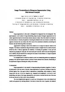
Similarly, the corresponding cloud model for object class 𝐶𝑜 can be also calculated. We take the original image in Figure 1(a) as a typical example, whose ground-truth image and the grayscale histogram are shown in Figures 1(b) and 1(c). We fix the optimal threshold 𝑡 = 214 according to its ground-truth image in Figure 1(b), and then the numerical characters of cloud models for background and object are calculated, respectively, that is, 𝐶𝑏 (60.6, 461.5, 111.7) and 𝐶𝑜 (249.1, 0.2, 91.8). Figure 1(d) demonstrates the joint distribution of cloud drops and its certainty degree. Cloud model has depicted the gray level distribution of the sample image, and it is an approximate normal distribution, or a generalized normal distribution, rather than a normal distribution. Furthermore, the grayscale distributions between background
4
Mathematical Problems in Engineering
(a)
(b)
1 0.03
0.9 0.8 Certainty degree 𝜇
0.025
Frequency
0.02 0.015 0.01
0.7 0.6 0.5 0.4 0.3 0.2
0.005
0.1 0 0
50
100 150 Grayscale
200
250
0
0
50
100 150 Grayscale
200
250
Background Cb
Object Co (c)
(d)
Figure 1: The sample image named irw10-000217: (a) the original image, (b) the ground-truth image, (c) the grayscale histogram, and (d) the cloud models for two classes.
and object must not be similar since the shapes of two cloud models are seriously different from Figure 1(d), as well as the ratio of these numerical characters. We will further analyze the difference in another section below. Once the cloud models are prepared, the remaining is to construct an appropriate criterion for image thresholding. Suppose the cloud model for the background class is 𝐶𝑏 (Ex𝑏 (𝑡), En𝑏 (𝑡), He𝑏 (𝑡)) and that of the object class is 𝐶𝑜 (Ex𝑜 (𝑡), En𝑜 (𝑡), He𝑜 (𝑡)); our criterion is related to the hyper-entropies He𝑏 (𝑡), He𝑜 (𝑡) of cloud models 𝐶𝑏 , 𝐶𝑜 . In an effort to eliminate the above limitation, we propose a novel criterion based on cloud model, which can be formulated as 𝐽 (𝑡) = max (He𝑜 (𝑡) , He𝑏 (𝑡)) .
(13)
Then the optimal threshold 𝑇 can be determined as follows: 𝑇 = arg min {𝐽 (𝑡)} . 𝑡∈[0,𝐿−1]
(14)
The segmented result by the proposed method is shown in Figure 2(a), from which one can observe that the cloud model-based method yields the acceptable performance, and the result image is closed with ground-truth image in Figure 1(b). To view the details, the evolution curve of function values is shown in Figure 2(b). With varied grayscale level, the function value increases steadily and achieves the maximum near 150 and then decreases dramatically. At the optimal gray level, the curve is with the minimal value, followed by a slight growth. It should be noted that the curve reaches max near 150, where the cloud models have little overlap (see Figure 1). In other words, this interval is full of chaos from the perspective of grayscale intensity, and the differences between the hyper-entropy of two cloud models are relatively highest. This means that one class achieves better partition while the other achieves worse. Maybe, these two classes even have similar standard deviation or population size in this condition. Unfortunately, this is not very compatible with the practical features of infrared images. As can be seen from
Mathematical Problems in Engineering
5 2000 1800 1600
Criterion values
1400 1200 1000 800 600 400 200 0
(a)
0
50
100 150 Grayscale
200
250
(b)
Figure 2: The segmented result of sample image by the proposed method: (a) the result image, (b) the cloud model-based function value.
(13) and (14), the new criterion actually attempts to divide an image into two parts with lower and similar hyper-entropy. Therefore, the classes of background and object have the higher intraclass similarity without distractions and certainly the lower interclass similarity. This is intuitively appealing as a good image segment. In ideal cases with two zero hyper-entropies, the two classes will yield bimodal Gaussian distribution, regardless of the population size. For the image in Figure 1(a), the segmented results by four traditional methods are shown in Figure 3, including Otsu, Hou, Li, and Xue. The result images in Figures 3(a), 3(b), and 3(d) by Otsu, Hou, and Xue almost completely misclassify the object pixels, and the Li method exhibits an acceptable result as shown in Figure 3(c), but there is still suffering from undersegmentation; the background pixels are misclassified into object, as labelled by a yellow rectangle. For reference, each evolution curve of function value is listed in Figure 1. The results by Otsu and Xue are totally wrong. Although the Hou method finds a faulty threshold, it is competitive, and its function value is very closed to the real optimal solution. With the modification of the Hou method, result by Li is more qualified, but the final threshold is still imperfect. To make an in-depth analysis on features of the sample image, we plot the histograms with 𝑦-axes on both left and right sides, as shown in Figure 4(a); the grayscale level versus frequency of background with 𝑦-axis is labelled on the left, while frequency of object is on the right. This image appears as a distinct unimodal grayscale distribution, and the peak ratio between the classes of background and object is very startling, which is about 300 : 1, which is high above tolerable ability of the Otsu, Hou, and Xue methods. Thus, the failure by these methods is a natural consequence. This is also a reason leading to the difference between each pair of parameters of cloud models, as mentioned in previous section. To observe whether or not the grayscale distributions of two classes satisfy Gaussian form, we use double Gaussian functions to fit the histograms of background and object,
respectively, and the fitting error rate is plotted in Figure 4(b). The grayscale distribution of background is more likely a Gaussian form, whose fitting error rate is smaller and acceptable. And the distributions are with difference variances, which is not satisfying the assumption of the Li method. Hence, the just passable result is produced by this method. Besides, this is another reason leading to the difference between cloud models. Furthermore, the evolution curves of function values by various methods are listed on semi-logarithmic coordinate, as shown in Figure 4(c). For simplicity, we only plot Xue’s curve with omitting the Otsu method, since these two methods achieve similar results and have no essential difference. Additionally, the Li method searches similar standard deviation, while our method searches similar hyper-entropy; then we plot variance difference and hyper-entropy difference for a clear comparison with a close magnitude. A threshold locating in the interval [180, 225] is more preferable. Li’s rule produces 𝑇 = 171, while ours produces 𝑇 = 213 obtaining a significant improvement. Of course, the pixels with grayscale value in [180, 225] are not very much. Hence, there seems to be so little difference between the visual results of Li and our method. Therefore, we will verify this point using various images and then further investigate the performance on target detection application, as shown in the following section. The quantitative comparison is also listed in Table 1, where ME denotes misclassification error and will be explained in Section 4. Our method yields the preferable result with the lowest misclassified pixels and the smallest ME value, since it can provide a more objective representation and accord with actual information of the image. Additionally, the running times by the methods are listed in Table 1. The proposed method, compared with the related methods, is also a competitive one from the perspective of time performance. 3.3. The Cloud Model-Based Algorithm. The proposed algorithm for cloud model-based infrared image thresholding
6
Mathematical Problems in Engineering 650 600
Criterion values
550 500 450 400 350 300
0
50
100
150
200
250
150 Grayscale
200
250
150
200
250
Grayscale (a)
2500
Criterion values
2000
1500
1000
500
0
50
100
0
50
100
(b)
600
Criterion values
500
400
300
200
100
0
Grayscale (c)
Figure 3: Continued.
Mathematical Problems in Engineering
7 18 17
Criterion values
16 15 14 13 12 11 10
0
50
100
150 Grayscale
200
250
(d)
Figure 3: The segmented results of sample image and the function values by various methods, including (a) Otsu, (b) Hou, (c) Li, and (d) Xue, respectively.
Table 1: Thresholds, misclassified pixels, ME values, and running times obtained by four traditional methods, Otsu, Hou, Li, and Xue, as well as the proposed method. irw10-000217 Threshold Misclassified pixels ME Running times (s)
Otsu 54 51534 0.6711 0.119775
Hou 42 59224 0.7711 0.121873
is as shown in Algorithm 1. The method firstly generates the cloud models corresponding to image background and object, respectively, and defines a novel threshold dependence criterion related with the hyper-entropy of these cloud models and then determines the optimal grayscale threshold by the minimization of this criterion. 3.4. Implementation and Computational Complexity. In Algorithm 1, there is a for loop with 𝐿 iterations, and each execution costs the time 𝑂(𝐿). Theoretically, the time complexity of the proposed algorithm is 𝑂(𝐿2 ). However, the proposed algorithm can be easily implemented by modifying the traditional methods, including Otsu and Hou. The efficient implementations for traditional methods are also applied equally to the cloud model-based technique. By comparison, the additional time cost is required to calculate the entropy of two classes, and calculations of the hyper-entropy only execute a subtraction as (12) showed. In sum, the time complexity of the proposed algorithm with efficient implementation is 𝑂(𝐿), approximately linear in the grayscale level 𝐿 of the original image. For an image with the size of 320 × 240, the time consumption is usually about 0.1 s in our practice.
Method Li 171 207 0.0027 0.122281
Xue 51 53957 0.7026 1.152522
Our method 213 15 0.0001 0.132543
4. Experimental Results 4.1. Experimental Setup. To demonstrate the efficiency of the proposed method, we conduct two groups of experiments, and seven methods are involved into comparison, including Kittler and Illingworth [19], Kapur et al. [20], Ramesh et al. [21], Otsu [7], Hou et al. [8], Li et al. [9], and Xue and Titterington [10]. The parameter setting is very important for performance evaluation. For a fair comparison, all are autoparameters or free parameters, but not from a guess. The latter five methods, including the Otsu, Hou, Li, and Xue method, as well as the proposed method, implemented by us, are based on the counts of the histogram, and the only parameter is the number of the bins when calculating the image histogram; we fixed it as 256, which is a conventional rule, so we can consider them as free parameters. The other three methods, including the Kittler, Kapur, and Ramesh method, are performed by the executable file from the public website maintained by Mehmet Sezgin [5] (http://mehmetsezgin.net/otimec.zip), which we cannot modify; these methods can be considered as autoparameters. The used data includes two groups. The partial data is composed of four images including different objects, and
8
Mathematical Problems in Engineering ×10−4
10
8 0.2
25 Frequency error rate (%)
8 Frequency
6 0.15 4
0.1
2
0.05
0
50
100 150 Grayscale
200
20 6 15 4 10 2
5
0
250
Background Object
50
100 150 Grayscale
200
250
Background Object (a)
(b)
103
T = 42
102 101 100
T = 171 T = 213
T = 51
0 15 30 45 60 75 90 105 120 135 150 165 180 195 210 225 240 255
Criterion values (log)
10
4
Grayscale Median-based deviation Histogram
Hyper-entropy difference Variance sum Variance difference (c)
Figure 4: The analysis of sample image: (a) histograms of background and object, (b) frequency error rate of background and object using Gaussian fitting, and (c) the semi-log plot of function values by various methods.
the original images and ground-truth images are shown in Figure 5, named airplane, person, boat, and star, respectively. The others come from Terravic Motion IR Database and can be registered to download from the website (http://vciplokstate.org/pbvs/bench/). We take four images as examples, named irw101, irw102, irin011, and irin012, respectively. The original images and ground-truth images are listed in Figure 6. Half of them are selected from irw10 with one subject entering the field of view (FOV) from the left, and the remaining are from irin01 with monitoring an indoor hallway. We quantify the performance of these methods by means of misclassification error (ME) [31]. Considering image segmentation as a pixel classification process, the percentage of pixel misclassification is a measure of discrepancy.
ME reflects the percentage of background pixels wrongly assigned to foreground and, conversely, foreground pixels incorrectly assigned to background. For the two-class segmentation problem, it can be expressed as [31] (𝐵 ∩ 𝐵 + 𝐹 ∩ 𝐹 ) ME = 1 − 𝑜 𝑡 𝑜 𝑡 , (𝐵𝑜 + 𝐹𝑜 )
(15)
where background and foreground are denoted by 𝐵𝑜 and 𝐹𝑜 for the ground-truth image and by 𝐵𝑡 and 𝐹𝑡 for the test image. 𝐵𝑜 ∩ 𝐵𝑡 is the number of background pixels rightly assigned to background, and 𝐹𝑜 ∩ 𝐹𝑡 vice versa. ME varies from 0 for a perfectly classified image to 1 for a totally wrongly classified image.
Mathematical Problems in Engineering
9
Input: the original image 𝐼. Output: the optimal threshold 𝑇 and the result image 𝑅. (1) For the original image 𝐼, obtain the initial information, such as the number of pixels 𝑁, the grayscale level 𝐿, and then calculate the histogram ℎ(𝑖). (2) Initialize the parameters, including the optimal criterion value 𝐽𝑚 and the optimal threshold 𝑇. 𝐽𝑚 ← +∞; 𝑇 ← 0. (3) for 𝑡 = 0 to 𝐿 − 1 do (4) Obtain the classes of background and object. 𝐵(𝑡) ← {𝑥 | 0 ≤ 𝐼(𝑥) ≤ 𝑡}; 𝑂(𝑡) ← {𝑥 | 𝑡 < 𝐼(𝑥) ≤ 𝐿 − 1}. (5) if 𝐵(𝑡) = 0 or 𝑂(𝑡) = 0 then (6) Eliminate the extreme cases. 𝐽(𝑡) ← +∞. (7) else (8) Calculate the standard deviations 𝜎𝑏 (𝑡), 𝜎𝑜 (𝑡) of background and object using (3). (9) if 𝜎𝑏 (𝑡) > 0 and 𝜎𝑜 (𝑡) > 0 then (10) Generate the cloud models for background and object using (10)–(12). 𝐶𝑏 ← (Ex𝑏 (𝑡), En𝑏 (𝑡), He𝑏 (𝑡)); 𝐶𝑜 ← (Ex𝑜 (𝑡), En𝑜 (𝑡), He𝑜 (𝑡)). (11) Calculate the criterion value according to (13). 𝐽(𝑡) ← max(He𝑜 (𝑡), He𝑏 (𝑡)). (12) else (13) Eliminate the extreme cases. 𝐽(𝑡) ← +∞. (14) end if (15) end if (16) if 𝐽(𝑡) < 𝐽𝑚 then (17) Swap the global optimum for the current best. 𝐽𝑚 ← 𝐽(𝑡); 𝑇 ← 𝑡. (18) end if (19) end for (20) Segment the image with the above threshold 𝑇, denoted as the result image 𝑅. {1 if 𝐼 (𝑥) > 𝑇 𝑅 (𝑥) = { {0 otherwise (21) return 𝑇, 𝑅. Algorithm 1: Cloud model-based method for infrared image thresholding.
Figure 5: The first group of test images: the first row is the original images and the second is ground-truth images—from left to right, named airplane, person, boat, and star, respectively.
10
Mathematical Problems in Engineering
Figure 6: The second group of test images: the first row is the original images and the second is ground-truth images—from left to right, named irw101, irw102, irin011, and irin012, respectively.
To ensure the highest possible accuracy, the ground truth was created entirely by hand using the GNU image manipulation program (GIMP) (http://www.gimp.org/), and no semiautomatic technique was used. This was also important to avoid potential bias to any algorithmic facet of the procedure used to create it. But it should be noted that creating a 100% pixel accurate ground truth is, in general, impossible, due to the ambiguity in the true positions of the border pixels. 4.2. Comparison on Infrared Image Thresholding. In this group of experiments, we compare the segmentation results on the infrared images. The seven methods are involved into the comparison. The visual comparisons are shown in Figures 7 and 8. Each test image consists of eight components from up to down, the segmentation results obtained by Otsu, Hou, Li, Xue, Kittler, Kapur, Ramesh, and the proposed method, respectively. The airplane image is relatively simple to segment; however Otsu, Hou, Xue, and Kittler cannot present valid results, and other methods provide good results. The quantitative comparisons are listed in Table 2. Results of the boat image demonstrate similar conclusion with the airplane image. For the person image, Li’s result is unsatisfied. For the star image, all these methods yield no good results, but only our segmented image is the closest to ground-truth image. Results of the second group images by various methods show the similar performance. For images irw101 and irw102, our method appears with the best results, followed by the Li method. But there are several misclassified blocks scattered in the background, which should impact the performance of the subsequent steps. For the last two images, our method suffers from oversegmentation, and the person is not that complete, and the other methods yield undersegmentation. In summary, by a visual evaluation, the experimental results of these images indicate the proposed method is effective to yield the approximately ideal results. The visual evaluation is, however, applicationindependent. For a more detailed portrait, quantitative comparisons of segmentation results yielded by various methods are listed in Table 2. The proposed method
outperforms other methods, obtaining the less misclassified pixels and demonstrating the lower ME values. In other words, the proposed method yields better segmentation by a quantitative evaluation. For the comparison purpose, the processing times of the proposed approach and other methods are also listed in Table 2. From this perspective, the proposed method is similar with the traditional Otsu method, as well as the Hou and the Li method, since the main time costs of all these methods lie in the calculation of the histogram and the scan of the gray level one by one. The time performance of these methods depends on the complexity of the histogram, rather than the image size. As a result, the time cost by each method is quite similar, even the different images by the various methods. It is noted that three methods, including the Kittler, the Kapur, and the Ramesh method, are performed by the executable file, as mentioned above. Thus, the running times of these three methods cannot be obtained. Then the processing times of the methods are omitted in Table 2. According to experimental experience, the involved methods belong to 1-D thresholding and very high efficiency, and the average time costs of these methods are all less than 2 s in our experiments. The comparison between the time cost of the existing methods and ours is not strictly necessary. Even so, the comparison on running time in Table 2 still indicates that the proposed method is efficient because our method runs with less time cost, and the segmented results are acceptable. In addition, Figure 9 shows a boxplot diagram that summarizes the misclassification error rate statistics of individual thresholding method applied on all selected images. As can be seen, the lowest median is achieved with our method, followed by the Li method and next the Ramesh method. For reference, the detail views of these three methods are also provided. The proposed method has also the smallest interval within ±1.5 IQR of the first/third quartiles (𝑄1 and 𝑄3). The Hou and Otsu methods provided, overall, less accurate results. These results demonstrate the high level of competitiveness of our method. 4.3. Results of Infrared Image with Noise. To further investigate the performance of the proposed methods under noisy
Mathematical Problems in Engineering
11
Figure 7: The first group of segmentation results applying the proposed method compared to selected algorithms. From left to right, named airplane, person, boat, and star. From up to down, the result images by Otsu, Hou, Li, Xue, Kittler, Kapur, Ramesh, and the proposed method, respectively.
12
Mathematical Problems in Engineering
Figure 8: The second group of segmentation results applying the proposed method compared to selected algorithms. From left to right, named irw101, irw102, irin011, and irin012. From up to down, the result images by Otsu, Hou, Li, Xue, Kittler, Kapur, Ramesh, and the proposed method, respectively.
environment, the irin011 image is involved into comparison. According to Table 2, eight methods gain the closest performance for the clean irin011 image. Hence, the image is used in this subsection. The original image is contaminated by Gaussian noise with zero mean, as well as salt and pepper noise. Each noise tests 20 images; that is, Gaussian noise is with variances in {0.01, 0.02, . . . , 0.20}, and salt and pepper
noise is with intensities in {0.01, 0.02, . . . , 0.20}. Since the noise contamination is a random process, we repeat the process of each variance or intensity 10 times and average the results. The ME values corresponding to various noises are shown in Figure 10. The proposed method performs lower ME values than the other methods for all the Gaussian noise images.
Mathematical Problems in Engineering
13
Table 2: Thresholds (𝑇), misclassified pixels (MP), ME values, and running times (RT) obtained by selected methods and the proposed method. Image Airplane 𝑇 MP ME RT (s) Person 𝑇 MP ME RT (s) Boat 𝑇 MP ME RT (s) Star 𝑇 MP ME RT (s) irw101 𝑇 MP ME RT (s) irw102 𝑇 MP ME RT (s) irin011 𝑇 MP ME RT (s) irin012 𝑇 MP ME RT (s)
Method Xue Kittler
Otsu
Hou
Li
Kapur
Ramesh
Our method
53 18312 0.2794 0.119895
44 23154 0.3533 0.125463
135 242 0.0036 0.121684
45 22666 0.3458 0.843127
34 26473 0.4039 —
117 201 0.0031 —
114 336 0.0051 —
133 234 0.0035 0.131788
108 27227 0.2801 0.119309
116 20663 0.2125 0.127476
160 1097 0.0112 0.121449
111 24365 0.2506 1.464618
154 963 0.0099 —
153 963 0.0099 —
154 963 0.0099 —
225 184 0.0018 0.133256
94 15630 0.5243 0.119085
75 22289 0.7477 0.124232
164 215 0.0072 0.120860
86 18963 0.6361 0.496241
146 895 0.0301 —
130 1652 0.0554 —
151 659 0.0221 —
207 317 0.0106 0.131623
113 47125 0.4224 0.119017
126 56676 0.5081 0.125376
121 54310 0.4868 0.121557
115 48266 0.4326 1.711368
35 32495 0.2912 —
153 76052 0.6817 —
119 58180 0.5215 —
83 14926 0.1337 0.133964
57 50669 0.6597 0.119579
44 59316 0.7723 0.126232
172 41 0.0005 0.121975
54 53397 0.6952 1.152923
103 3252 0.0423 —
153 124 0.0016 —
137 642 0.0083 —
210 4 5.21E − 05 0.133889
56 51369 0.6688 0.119248
44 58720 0.7645 0.125052
169 55 0.0007 0.122033
52 54401 0.7083 1.149296
103 3080 0.0401 —
153 124 0.0016 —
137 626 0.0081 —
212 14 0.0001 0.132815
136 567 0.0073 0.119136
232 849 0.0111 0.125602
192 655 0.0085 0.121678
60 30066 0.3914 1.156888
86 2136 0.0278 —
102 955 0.0124 —
118 955 0.0124 —
217 754 0.0098 0.132685
66 28185 0.3669 0.118951
241 117 0.0015 0.125435
194 179 0.0023 0.121646
64 31137 0.4054 1.165576
0 75017 0.9767 —
119 635 0.0082 —
127 635 0.0082 —
220 109 0.0014 0.135214
The Kapur method ranks the second, followed by the Ramesh method and the Li method with a little difference. The other four methods, including the Otsu, the Hou, the Xue, and the Kittler method, show a poorer performance to Gaussian noise. On the other hand, the proposed method exhibits an acceptable performance under the condition contaminated by the salt and pepper noise, which is similar with the Otsu, the Hou, and the Li method. The Kittler method comes
next, while the Kapur and the Ramesh methods are invalid under this condition. Coincidently, these two methods show a better performance in the above round. Unfortunately, the Xue method is far from satisfactory under the conditions of both Gaussian noise and Salt and pepper noise. In general, the quantitative comparison with various noisy images suggests that our method is more robust to noise, especially under the condition contaminated by the Gaussian noise.
14
Mathematical Problems in Engineering 1
×10−3
0.9
×10 0.02 15 0.015 10 0.01 0.005 5 Ramesh 0
10
0.8
5
Values
0.7 0
0.6
Li
−3
Table 3: The configuration parameters for simulated data. Data set 𝐷1 𝐷2
|𝐵| 64512 65280
|𝑂| 1024 256
𝜇𝑏 90 90
𝜎𝑏2 30 30
𝑀1𝑏 4 4
𝜇𝑜 120 140
𝜎𝑜2 30 30
𝑀1𝑜 4 4
0.5 Ours
0.4
method, and the last is the extension of cloud model and its application.
0.3 0.2 0.1 0 Otsu
Hou
Li
Xue
Kittler Kapur Ramesh Ours
Figure 9: Boxplot of misclassification error rates (ME) by various methods, including Otsu, Hou, Li, Xue, Kittler, Kapur, Ramesh, and the proposed method.
4.4. Application on Infrared Image Target Detection. In this group of experiments, we apply the proposed method into infrared image target detection. By the way, six methods, including Otsu, Hou, Xue, Kittler, Kapur, and Ramesh, have inevitable weakness for infrared images according to the previous section; thus these methods are not included in the comparison. We only compare Li’s results with ours. The infrared image sequence comes from irw10, number 000220 to number 000470. One subject walks across FOV from left to right and is sheltered in two places. The processing steps are (1) segmenting the images by two methods, (2) generating the minimum bounding rectangle of object, and (3) then overlying the original images and converting the result image sequences into videos. The result videos in this subsection are included in the supplementary files (see Appendix B). Our result presents better performance without any preprocessing or postprocessing, although there exist two images with poor segmentation, where the shelter appears. Of course, we must objectively point out that our method may lead to slight oversegmentation in some cases, which does not affect target detection substantially. Our method mainly aims at the infrared image thresholding, and other postprocessing steps can be introduced into our method to improve the performance if involving target detection. The Li method provides just passable results, but it should suffer undersegmentation in most cases and even seriously degrade the performance. By comparison, our cloud model-based method performs a compelling performance in both image thresholding and target detection.
5. Discussions In this section, we discuss four problems: one is the relationship between our method and related methods, as well as the theoretical principle or foundation, next is applicability for infrared images, followed by the limitation of the proposed
5.1. Relations with Other Methods. Type-2 fuzzy set is defined by lower membership function and upper membership function. Similarly, cloud model is approximatively related by lower boundary 𝜇LB (𝑢) = exp(−(𝑢 − Ex)2 /2(En − 3He)2 ) (LB) and upper boundary 𝜇UB (𝑢) = exp(−(𝑢 − Ex)2 /2(En + 3He)2 ) (UB). But the region bounded by LB and UB is uncertainty, which is determined by He. In other words, cloud model has no clear boundary, but it is with a stable tendency (i.e., the expected curve 𝜇𝐸 (𝑢) = exp(−(𝑢 − Ex)2 /2En2 )), as shown in Figure 11. Li’s method is motivated by the isoperimetric graph partitioning [32], in which the intraclass similarities of object and background are measured by the sum of degrees of their corresponding vertices, while the interclass similarity is measured by a cut of the graph. From this perspective, one can also take the hyper-entropy as the intraclass similarity instead of vertices’ degree sum. The standard deviation is a common statistical measure representing degree of deviations between mean and individuals, and He is as the second-order or higher-order standard deviation. Therefore, He is a higherorder statistical measure representing degree of deviations between mean and individuals. Accordingly, He can also be used to measure intraclass similarity of each class in image thresholding. Thus, the cloud model-based method is equivalent to the isoperimetric constant when omitting interclass similarity of object and background, and the proposed criterion is equivalent to Li’s equation in some cases with En𝑏 (𝑡) = 0 and En𝑜 (𝑡) = 0, and they are approximate in many cases with smaller En𝑏 (𝑡) and En𝑜 (𝑡). For an extreme comparison, we randomly build two simulated data sets, denoted by 𝑆1 , 𝑆2 . The data in different sets correspond to pixel intensities in different types of virtual image of two groups (i.e., the background and the objects). The size of image 𝑁 = 256 × 256, and the number of background pixels is denoted by |𝐵|, while that of object is |𝑂| = 𝑁 − |𝐵|. The statistical parameters, including the mean, 𝜇𝑏 , 𝜇𝑜 , the variance, 𝜎𝑏2 , 𝜎𝑜2 , and the first-order central moment, 𝑀1𝑏 , 𝑀1𝑜 , are listed in Table 3. Since intensities are integers in the range [0, 𝐿 − 1], we round the simulated data into [0, 𝐿 − 1]. The segmented results are shown in Figure 12. With a larger entropy of classes (En𝑜 , En𝑏 ≈ 5), the results by our method are clearly different from Li’s results. Our method achieves good results, while Li’s method generates invalid results (completely misclassifying the background or the objects). Li’s method is unexpectedly inferior to the other methods, even though the assumption of the equal size class
Mathematical Problems in Engineering
15
1.0
0.4 0.3
0.6 ME value
ME value
0.8
0.4 0.2
0.2 0.1
0.0
0.0 0.00
0.05
0.10 0.15 Noisy variance
0.20
0.25
0.05
0.10 0.15 Noisy intensity
Otsu Hou Li Xue
Kittler Kapur Ramesh Ours
Otsu Hou Li Xue
0.00
(a)
0.20
0.25
Kittler Kapur Ramesh Ours (b)
Figure 10: The overall results for the irin011 image with noise: (a) total curves for the images corrupted by Gaussian noise of different variances, (b) total curves for the images corrupted by Salt and pepper noise of different intensities.
0.7 0.6
Frequency
0.5 0.4
Determined by He 0.3 0.2 0.1 0 60
80
100
Cloud drops Expectation curve
120 Grayscale
140
160
180
Lower boundary Upper boundary
Figure 11: The comparative schematic diagram.
for these traditional methods (e.g., the Otsu method) is not satisfied. 5.2. Applicability for Infrared Images. We confine the proposed method to infrared image thresholding, and there are two main reasons: (1) Our new criterion actually attempts to divide an image into two parts with lower and similar hyper-entropy, even higher-order entropy. Thus, the proposed method, especially the statistical criterion, is only suitable for a special histogram from the point of view of mathematical statistics, as discussed in the above subsection.
Almost all of infrared images have the statistical properties. Therefore, the proposed method is more suitable for applying to infrared images, since the infrared images have the special features more observably and more directly, especially for those infrared images with small targets. (2) The cloud model-based method is inspired by the Li method, which is specific for infrared images. Hence, the comparison is more meaningful with the same application. Compared with the Li method, our method improves attention to detail in target detection for infrared images. Thus, the proposed method is also positioned in specific for infrared images. Of course, our method can be also applied to the gray level images with similar statistical features, since the method is proposed to process the histogram only, but not the type of images. In fact, the proposed method performed well in the above subsection, in which there are simulated data sets, not infrared images. But we still think one cannot find out other types of images with the special features, which is more suitable than the infrared images. In other words, our method would generally achieve better performance by applying to infrared images rather than gray level images. Theoretically, another statistical criterion can be provided for gray level images which are more appropriate than the infrared images. Unfortunately, this criterion is still open and to be further investigated. Nevertheless, our method does not want to apply to all images. Meanwhile, we cannot do so, since each technique has both strengths and weaknesses. 5.3. The Limitation. In general, our method demonstrates good performance, both efficiency and effectiveness. Nonetheless, each algorithm has its advantages and disadvantages. None is generally applicable to all images; our method is no exception. The proposed method belongs to a special type of statistical approach, and it takes the histogram as the
16
Mathematical Problems in Engineering 3000 2500 2000 1500 1000 500 0
2500 2000 1500 1000 500 0 0
50 100 150 200 250
0
50 100 150 200 250
Figure 12: The results of simulated data applying the proposed method compared to selected algorithms. The simulated images and histograms are in the first row, and result for each image consists of two rows. From left to right, from up to down, the result images by Li, the proposed method, Otsu, Hou, Xue, Kittler, Kapur, and Ramesh, respectively.
fundamental basis; the division of background and object pixels depends on the statistical feature reflected by the image. The proposed cloud model has a certain capacity of processing uncertainty, when a small number of the object pixels are disguised as the background pixels from the point of view of the grayscale values. But it is never omnipotent, and when the statistical features of the object pixels in images were influenced seriously, the proposed method would suffer the oversegmentation. In extreme cases, the results would be unsatisfied, even wrong. For example, the proposed method currently cannot deal with texture; thus it does not work well if involved into the gray level images with texture, which can be easily processed by the other specific methods. In this view, our method is more specified for the infrared images, since it is difficult to reflect the target texture information by infrared images. Additionally, incorporating semantics into image segmentation and scene understanding is recently a new trend. The lack of introducing semantics information
is another limitation of the proposed method, although the statistical method is simple and feasible. 5.4. The Extension. In this paper, the cloud model, 2nd-order essentially, uses three numerical characteristics Ex, En, He to represent the classes of background and objects pixels. Furthermore, cloud model can generate the next-order entropy, which is the higher-order cloud model, if hyperentropy is not enough to support or represent the statistical properties of a given image. Theoretically, the entropy of cloud model has the ability of an infinite extension. Wang et al. [17] have proposed the 𝑝th-order generic normal cloud model, which is expressed by 𝑝 + 1 numerical characteristics. The recursive definition of the 𝑝th-order normal cloud is the popularization of the 2nd-order normal cloud and the normal distribution. The 𝑝th-order normal cloud has the unimodal and long-tail property, and then it is able to represent a power-law distribution [33]. From normal distribution
Mathematical Problems in Engineering to power-law distribution, cloud model has flexibility to represent the classes of background and objects in images. For the application on image thresholding using higherorder cloud model, only one extra step is inserted as preprocessing of the proposed method. A possible way is to search the optimal order 𝑝 from 1 to 𝑝𝑚 (the right bound of order) so as to achieve that 𝑝th-order normal cloud can represent the two classes with the least error, compared with the original histogram. The step is easy to implement, but the searching process of 𝑝 should take the additional time. Theoretically, with a larger 𝑝𝑚 , the representing error is less, and the segmented results are more perfect, while the time cost is more. In practice, how to keep a balance between them is really a challenge. From the perspective of time complexity, we only use 2nd-order cloud model in this paper, which is a special case of the 𝑝th-order normal cloud model.
6. Summary and Conclusion In this paper, a new algorithm for infrared image thresholding has been described. We analyze the rationale of the proposed approach. Cloud model is introduced into the representation of image background and objects, as named by cloud model with three parameters (Ex, En, He). The method possesses only one free parameter, the hyper-entropy He, over which a criterion function is evaluated and the optimal threshold can be determined by optimizing the function value. A comparison with seven other thresholding methods has been presented. The results indicate that the proposed method is effective and efficient and highly competitive with other popular methods. Like any other methods, the proposed method maybe also has limitations and suffers from oversegmentation in some cases, which will be further considered and essentially improved in our future research.
17
[3]
[4]
[5]
[6]
[7]
[8]
[9]
[10]
[11]
[12]
[13]
Competing Interests The authors declare that they have no competing interests.
Acknowledgments This work was partially supported by the National Natural Science Foundation of China under Grant (nos. 61402399, 41501378), by National Key Basic Research and Development Program (no. 2012CB719903), by Foundation for Distinguished Young Teachers in Higher Education of Guangdong, China (no. YQ2014117), and by the Foundation of Humanities and Social Sciences Research in Ministry of Education, China (no. 14YJCZH161).
[14]
[15]
[16]
[17] [18]
References [1] E. Cuevas, A. Gonz´alez, F. Fausto, D. Zald´ıvar, and M. P´erezCisneros, “Multithreshold segmentation by using an algorithm based on the behavior of locust swarms,” Mathematical Problems in Engineering, vol. 2015, Article ID 805357, 25 pages, 2015. [2] A. N. Benaichouche, H. Oulhadj, and P. Siarry, “Improved spatial fuzzy c-means clustering for image segmentation using PSO initialization, Mahalanobis distance and post-segmentation
[19]
[20]
correction,” Digital Signal Processing, vol. 23, no. 5, pp. 1390– 1400, 2013. Y. Zou, H. Liu, and Q. Zhang, “Image bilevel thresholding based on stable transition region set,” Digital Signal Processing, vol. 23, no. 1, pp. 126–141, 2013. Y. Zou, F. Dong, B. Lei, S. Sun, T. Jiang, and P. Chen, “Maximum similarity thresholding,” Digital Signal Processing, vol. 28, no. 1, pp. 120–135, 2014. M. Sezgin and B. Sankur, “Survey over image thresholding techniques and quantitative performance evaluation,” Journal of Electronic Imaging, vol. 13, no. 1, pp. 146–168, 2004. K. Charansiriphaisan, S. Chiewchanwattana, and K. Sunat, “A comparative study of improved artificial bee colony algorithms applied to multilevel image thresholding,” Mathematical Problems in Engineering, vol. 2013, Article ID 927591, 17 pages, 2013. N. Otsu, “A threshold selection method from gray-level histogram,” IEEE Transactions on Systems, Man, and Cybernetics, vol. 9, no. 1, pp. 62–66, 1979. Z. Hou, Q. Hu, and W. L. Nowinski, “On minimum variance thresholding,” Pattern Recognition Letters, vol. 27, no. 14, pp. 1732–1743, 2006. Z. Li, C. Liu, G. Liu, X. Yang, and Y. Cheng, “Statistical thresholding method for infrared images,” Pattern Analysis and Applications, vol. 14, no. 2, pp. 109–126, 2011. J.-H. Xue and D. M. Titterington, “Median-based image thresholding,” Image and Vision Computing, vol. 29, no. 9, pp. 631–637, 2011. T. Wu, J. Xiao, K. Qin, and Y. Chen, “Cloud model-based method for range-constrained thresholding,” Computers & Electrical Engineering, vol. 42, pp. 33–48, 2015. T. Wu and K. Qin, “Comparative study of image thresholding using type-2 fuzzy sets and cloud model,” International Journal of Computational Intelligence Systems, vol. 3, supplement 1, pp. 61–73, 2010. H. Deng, Y. Wei, and M. Tong, “Small target detection based on weighted self-information map,” Infrared Physics and Technology, vol. 60, pp. 197–206, 2013. Z.-J. Feng, X.-L. Zhang, L.-Y. Yuan, and J.-N. Wang, “Infrared target detection and location for visual surveillance using fusion scheme of visible and infrared images,” Mathematical Problems in Engineering, vol. 2013, Article ID 720979, 7 pages, 2013. D. Li, C. Liu, and W. Gan, “A new cognitive model: cloud model,” International Journal of Intelligent Systems, vol. 24, no. 3, pp. 357–375, 2009. D. Li and Y. Du, Artificial Intelligence with Uncertainty, Chapman and Hall/CRC, Boca Raton, Fla, USA, 2007, http://www.crcpress.com/product/isbn/9781584889984. G. Wang, C. Xu, and D. Li, “Generic normal cloud model,” Information Sciences, vol. 280, pp. 1–15, 2014. K. Qin, K. Xu, F. Liu, and D. Li, “Image segmentation based on histogram analysis utilizing the cloud model,” Computers and Mathematics with Applications, vol. 62, no. 7, pp. 2824–2833, 2011. J. Kittler and J. Illingworth, “Minimum error thresholding,” IEEE Transaction on System Man Cybernetics, vol. 19, no. 1, pp. 41–47, 1986. J. Kapur, P. Sahoo, and A. Wong, “A new method for graylevel picture thresholding using the entropy of the histogram,” Computer Graphics and Image Processing, vol. 34, no. 11, pp. 273– 285, 1985.
18 [21] N. Ramesh, J.-H. Yoo, and I. K. Sethi, “Thresholding based on histogram approximation,” IEE Proceedings: Vision, Image and Signal Processing, vol. 142, no. 5, pp. 271–279, 1995. [22] K. Qin, D. Li, T. Wu, Y. Liu, G. Chen, and B. Cao, “Comparative study of type-2 fuzzy sets and cloud model,” in Proceedings of the 5th International Conference on Rough Set and Knowledge Technology (RSKT ’10), pp. 604–611, Springer, Berlin, Heidelberg, 2010. [23] X. Wu, G. Guo, and Z. Bai, “Cloud model-based energy management strategy for parallel hybrid vehicles,” Journal of Control Science and Engineering, vol. 2015, Article ID 141654, 7 pages, 2015. [24] H. Liu, F. Yi, and H. Yang, “Adaptive grouping cloud model shuffled frog leaping algorithm for solving continuous optimization problems,” Computational Intelligence and Neuroscience, vol. 2016, Article ID 5675349, 8 pages, 2016. [25] P. Lv, L. Yuan, and J. Zhang, “Cloud theory-based simulated annealing algorithm and application,” Engineering Applications of Artificial Intelligence, vol. 22, no. 4-5, pp. 742–749, 2009. [26] E. Torabzadeh and M. Zandieh, “Cloud theory-based simulated annealing approach for scheduling in the two-stage assembly flowshop,” Advances in Engineering Software, vol. 41, no. 10-11, pp. 1238–1243, 2010. [27] S. Jia and B. Mao, “Research on CFCM: car following model using cloud model theory,” Journal of Transportation Systems Engineering and Information Technology, vol. 7, no. 6, pp. 67–73, 2007. [28] L. Liao and W. W. Guo, “Incorporating utility and cloud theories for owner evaluation in tendering,” Expert Systems with Applications, vol. 39, no. 5, pp. 5894–5899, 2012. [29] J. M. Mendel, “Type-2 fuzzy sets and systems: an overview,” IEEE Computational Intelligence Magazine, vol. 2, no. 1, pp. 20– 29, 2007. [30] W.-L. Hung and M.-S. Yang, “Similarity measures between type2 fuzzy sets,” International Journal of Uncertainty, Fuzziness and Knowledge-Based Systems, vol. 12, no. 6, pp. 827–841, 2004. [31] A. Z. Arifin and A. Asano, “Image segmentation by histogram thresholding using hierarchical cluster analysis,” Pattern Recognition Letters, vol. 27, no. 13, pp. 1515–1521, 2006. [32] L. Grady and E. L. Schwartz, “Isoperimetric graph partitioning for image segmentation,” IEEE Transactions on Pattern Analysis and Machine Intelligence, vol. 28, no. 3, pp. 469–475, 2006. [33] G.-Y. Wang, C.-L. Xu, Q.-H. Zhang, and X.-R. Wang, “p-order normal cloud model recursive definition and analysis of bidirectional cognitive computing,” Chinese Journal of Computers, vol. 36, no. 11, pp. 2316–2329, 2013.
Mathematical Problems in Engineering
Advances in
Operations Research Hindawi Publishing Corporation http://www.hindawi.com
Volume 2014
Advances in
Decision Sciences Hindawi Publishing Corporation http://www.hindawi.com
Volume 2014
Journal of
Applied Mathematics
Algebra
Hindawi Publishing Corporation http://www.hindawi.com
Hindawi Publishing Corporation http://www.hindawi.com
Volume 2014
Journal of
Probability and Statistics Volume 2014
The Scientific World Journal Hindawi Publishing Corporation http://www.hindawi.com
Hindawi Publishing Corporation http://www.hindawi.com
Volume 2014
International Journal of
Differential Equations Hindawi Publishing Corporation http://www.hindawi.com
Volume 2014
Volume 2014
Submit your manuscripts at http://www.hindawi.com International Journal of
Advances in
Combinatorics Hindawi Publishing Corporation http://www.hindawi.com
Mathematical Physics Hindawi Publishing Corporation http://www.hindawi.com
Volume 2014
Journal of
Complex Analysis Hindawi Publishing Corporation http://www.hindawi.com
Volume 2014
International Journal of Mathematics and Mathematical Sciences
Mathematical Problems in Engineering
Journal of
Mathematics Hindawi Publishing Corporation http://www.hindawi.com
Volume 2014
Hindawi Publishing Corporation http://www.hindawi.com
Volume 2014
Volume 2014
Hindawi Publishing Corporation http://www.hindawi.com
Volume 2014
Discrete Mathematics
Journal of
Volume 2014
Hindawi Publishing Corporation http://www.hindawi.com
Discrete Dynamics in Nature and Society
Journal of
Function Spaces Hindawi Publishing Corporation http://www.hindawi.com
Abstract and Applied Analysis
Volume 2014
Hindawi Publishing Corporation http://www.hindawi.com
Volume 2014
Hindawi Publishing Corporation http://www.hindawi.com
Volume 2014
International Journal of
Journal of
Stochastic Analysis
Optimization
Hindawi Publishing Corporation http://www.hindawi.com
Hindawi Publishing Corporation http://www.hindawi.com
Volume 2014
Volume 2014