clusiVAT: A Mixed Visual/Numerical Clustering Algorithm for Big Data Dheeraj Kumar Marimuthu Palaniswami
Christopher Leckie James C. Bezdek
Sutharshan Rajasegarar
CIS, U. of Melbourne Victoria 3010, Australia
[email protected] [email protected]
EEE, U. of Melbourne Victoria 3010, Australia {dheerajk@student., palani@, sraja@} unimelb.edu.au
AbstractRecent algorithmic and computational improvements have reduced the time it takes to build a minimal spanning tree (MST) for big data sets. In this paper we compare single linkage clustering based on MSTs built with the FilterKruskal method to the proposed clusiVAT algorithm, which is based on sampling the data, imaging the sample to estimate the number of clusters, followed by non-iterative extension of the labels to the rest of the big data with the nearest prototype rule. Numerical experiments with both synthetic and real data confirm the theory that clusiVAT produces true single linkage clusters in compact, separated data. We also show that single linkage fails, while clusiVAT finds high quality partitions that match ground truth labels very well. And clusiVAT is fast: it recovers the preferred c = 3 Gaussian clusters in a mixture of 1 million twodimensional data points with 100% accuracy in 3.1 seconds. Keywords-Cluster Analysis, Pattern Linkage, Big Data, Filter-Kruskal MST.
Recognition,
Single
I. INTRODUCTION AND RELATED WORK Clustering is the problem of partitioning a set of unlabeled objects O = {o1, …, on} into c groups of similar objects, 1 < c < n. Many texts describe various approaches to clustering [1-6]. When oi ∈ O is represented by x i ∈ ℜ p , X = {x1,…,xn} is a feature data representation of O. The k-th component of xi is the kth feature or attribute of oi. When relational values between pairs of objects are available, we have relational data. The relation ρ on O×O is represented by a square matrix Rn×n = [rij], where rij = ρ(oi,oj) is the relationship between oi and oj, 1 ≤ i, j ≤ n. X can be converted into dissimilarity data D n×n = [d ij ] = x i − x j using any norm on ℜ p . Similarity
Timothy C. Havens ECE/CS, Michigan Tech U., Houghton, MI 49931, USA
[email protected]
perhaps first noted in [1]. When every pair of vertices in G is connected, the MST is often called the Euclidean MST (EMST), a somewhat misleading terminology, since the edge weights need not be Euclidean distances (nor even metric distances). Once a MST is begun, SL proceeds by connecting a next closest vertex to the current edge set until the tree is formed. Clusters are found by cutting edges in the tree: cut the largest edge to divide the vertex set into c = 2 connected spanning forests; cut the next largest edge to obtain c = 3 SL clusters, etc. Consequently, SL is at its best when clusters in the data form well separated geometric strings or chains. Conversely, SL becomes increasingly unreliable as the clusters become more and more voluminous and cloud-like. However, there have been many successful applications of SL in various contexts. Lacy and Cole [7] discuss discovery of dark matter haloes in astronomy with SL; Moshtaghi et al. [8] use SL for anomaly detection in wireless sensor networks; Wilbik et al. [9] use SL to cluster segments of time series associated with sensor-based monitoring of elder patients; and of course, the dendrograms that are part and parcel of SL are prominent in many, many applications of numerical taxonomy [10]. So, while SL has very clear limits, it is still worthwhile to find scalable versions of it that efficiently process big data.
data S are always convertible to dissimilarity data D using simple transformations such as D = [1]-S.
How big is "Big Data?". Big Data encompasses four main problems: volume, velocity, variety, and veracity. In this paper, we are focusing on the volume of Big Data, namely the storage limitations of working memory on a computational platform. So, what is the volume of Big Data? Facebook alone processes 500+ terabytes (TB) of data per day. The Library of Congress recently cataloged over 170 billion tweets - every tweet since Twitter started. Is this big? For us, data is big if it cannot be loaded and processed in internal memory.
Single linkage (SL) clustering in dissimilarity data D has been used for nearly a century. Gower and Ross [1] attribute the basic idea underlying SL to Czekanowski [2]. The SL model is intimately related to the minimal spanning tree (MST) of an undirected, weighted graph G(V, E) whose vertex set is V (|V|=n) and edge set is E (|E|=m). The MST problem and an algorithm for solving it were reported in 1926 by Boruvka [3]. The algorithms that are used most often for construction of the MST are Kruskal's 1956 algorithm [4], and Prim's 1957 algorithm [5]. The connection between SL and the MST was
Recent advances in accelerating computation of the MST (and, as a by-product, SL clustering) for big data include the Filter-Kruskal (FK) algorithm [11], and the DualTreeBoruvka (DTB), algorithm of March et al. [12]. The algorithms in [11] and [12] concentrate on fast MSTs, and since they are exact, single linkage partitions can be extracted from their MSTs. The first scalable SL algorithm for big data that we know of is clustering with scalable visual assessment of tendency (clusVAT) algorithm reported by Havens et al. in [13], where it was called sVAT-SL. This scheme is based on sampling
[
]
followed by non-iterative extension to the non-sampled vertices using a nearest prototype classifier. This method produces exact SL partitions for a small subclass of problems, but for the large majority of possible inputs, clusVAT abandons the SL format and strikes out on its own. CPU times are at least as good as those of other internal MST schemes, and this method has a built in visualization mechanism for estimating the "best" number of SL clusters to retain. Most of the fast MST papers do not consider ways and means for deciding which set of SL clusters are most desirable (viz., cluster validation), so this is an added advantage for clusiVAT. But to date, there has been no comparison of clusiVAT to SL clusters built with fast MST schemes. The objective of this note is to compare the quality and speed of clusiVAT partitions to SL partitions of big data extracted from FK MSTs. Next, we give a brief description of the two algorithms. II. THE CLUSIVAT AND FK ALGORITHMS Visual representation of structure in unlabeled dissimilarity data using reordered dissimilarity images (RDIs) began in 1909 [2]. The intensity of each pixel in an RDI corresponds to the dissimilarity between the addressed row and column objects. An RDI is "useful" if it highlights potential clusters as a set of "dark blocks" along its diagonal. Each dark diagonal block represents a group of objects that are fairly similar. Our approach to fast clustering in big data is rooted in a method called visual assessment of clustering tendency (VAT, [14]). VAT reorders an input dissimilarity matrix D→D* using a modification of Prim's algorithm, and displays a grayscale image I(D*). VAT has proven its value in various applications [8, 9], but suffers from size limitations. Hardware and software limit the input data D n = D n×n to n ≈ O(104). Scalable VAT (sVAT) was introduced in [15] to overcome these limitations for big data, represented here by the N × N matrix DN , where N is arbitrarily large. sVAT finds a sample D n ⊂ D N and offers sVAT(D n ) = I(D*n ) as a viewable approximation to the big, intractable and unVATable image VAT(D N ) = I(D *N ) . These algorithms are well documented in the literature. Fig. 1, which replicates Figs. 2, 6 in [15], shows how this works. Figure (1a) is a scatterplot of a small (N = 5,000) set of clusters X drawn from a c=3 component Gaussian mixture. These object data were converted to distance matrix D using the Euclidean norm. Three dark diagonal blocks in the VAT image of XN seen in view 1(b) suggest that c = 3 is a good choice. View 1(c) is the sVAT image of D built from 2% of the data in roughly 0.2% of the time needed for the full image, and this image shows essentially the same thing. Fig. 1(d) shows a similar data set with N=100,000 points. Now D ≈ O(1010), so there is no VAT image, indicated in Fig. 1(e) by ?. Fig. 1(f) is the sVAT image for these data built with 500/100,000=0.5% of the data in a few seconds. This demonstrates the visual basis of clusiVAT and the speed at which it operates on big data. While VAT/sVAT are useful, much sharper images can usually be obtained using recursive improved VAT (iVAT, [16]) and by direct extension, its scalable form siVAT. iVAT is a simple modification of VAT that begins with feature
(a) Object data XN
(b)VAT; N = 5,000
(c) sVAT; n =100
? (d) Object Data Set XN
(e) VAT; N = 100,000
(f) sVAT; n = 500
Fig. 1. VAT and sVAT images of Gaussian Clusters
extraction based on replacing the input distances D = [dij] with geodesic distances D' = [d’ij]. Fig. 2 illustrates the improvement to a VAT assessment image that can be made by this transformation. The data set XBS shown in view 2(a) has five visually apparent clusters. The VAT image of this data built using Euclidean input distances is shown in Fig. 2(b) fails to offer us a very strong suggestion that these data do possess five clusters. Fig. 2(c) is the iVAT image of this data set which clearly suggests, by the five dark blocks along its diagonal, that we should look for c = 5 clusters in the data.
(a) Object data XBS
(b)VAT image
(c) iVAT image
Fig. 2. VAT and iVAT images of a data set XBS with c = 5 clusters c
Let X = U X i be the c clusters in partition U, and let d be i=1
any metric on ℜ p × ℜ p . ∆(X i ) = max{d( x, y) : x, y ∈ X i } is the diameter of Xi. The set distance between Xi and Xj is δ(X i , X j ) = min{d(x, y) : x ∈ X i , y ∈ X j} . This condition triggers the merger of Xi and Xj by agglomerative SL, so this set distance is sometimes called the SL distance. Dunn [17] defined the separation index for U as
Dunn proved that X can be clustered into a compact, separated (CS) c-partition if and only if max{VD(U;X)} > 1. The connection between aligned partitions, single linkage clusters, Dunn's index and iVAT is discussed in [18]. It is shown in [13] that clusVAT (the father of clusiVAT, which
was called sVAT-SL in [13]) produces exact SL clusters for any X or D that can be partitioned into CS clusters. Since the version of iVAT built by recursion in [16] preserves the VAT ordering, siVAT and sVAT share the same theory. When we cannot confirm the CS property for input data, SL replication by sVAT/siVAT is not guaranteed. In this case, clusiVAT becomes a new clustering model and algorithm. How many data sets have CS clusters? Not so many. This important fact restricts data sets for which clusiVAT is exact, but it can be applied to arbitrarily big data, hence its utility. Pseudo code for the algorithms is given in Fig. 3. To save space we indicate "or" by "/" in Fig. 3. Skipping iVAT results in clusVAT; running iVAT results in clusiVAT. Using iVAT upgrades the algorithm and its acronym to clusiVAT. We will discuss only clusiVAT in the remainder of this note.
Filter-Kruskal (FK) [11] alters the qKruskal algorithm [19], which combines Kruskal with Quicksort. qKruskal partitions the edges into light and heavy subsets, recurses on the light edges first, and then on the heavy edges if necessary. FK adds early filtering to qKruskal, sorting out "heavy" edges in components of the current forest that cannot contribute to the MST. FK is the last algorithm in Fig. 3. In the pseudocode, T is a set of already known MST edges, P is the partition of V induced by T. The FK procedure is initialized with T= Ø, U = [1 1 ... 1]. The asymptotic run time complexity of FK for arbitrary big graphs (|V|=N, |E|=M) with random edge weights is O(M+ NlogN•log(M/N)). The complexity of clusiVAT is (i) vectors X N ⊂ ℜ p ⇒ O (max{pc′N, pn2 , (n + c′)2}) ; (ii) dissimilarity data D N ⊂ ℜ NN ⇒ O (max{c′N, (n + c′)2}). clusiVAT does not asymptotically scale linearly with N, because n can be written as a constant multiple of N (however, the constant is usually