Cluster Cores-based Clustering for High Dimensional Data
Recommend Documents
Oracle Data Mining Technologies. 10 Van de Graaff Drive. Burlington, MA 1803, USA. Abstract. Clustering large data sets of high dimensionality has always ...
The PoCluster is organized in DAG with subset relationship .... ever, unlike low dimensional data where each of the attributes is considered equally ..... Given the data matrix D, as defined above, we define a row cluster as a subset of ...... For ex
algorithms [Goldberg, 1989] include a class-related randomized, population- based heuristics search ... When we are searching for the best attribute subset, we must choose the same number of clusters ..... IOS Press, 2002. [Liu and Motoda ...
possible [5, 25, 22, 17]. However, these .... are in s-dim subspace of noise, orthogonal to the r-dim relevant ... rotations such as U and V in PCA, RT R = RT R = Ik .... that qk will be close to the µk centers if they are rea- sonably ... data into
Eastern Virginia Medical School, Norfolk, VA 23507, USA. Received 9 September 2004; revised 10 ... [email protected]. This is an open access article ...
Proceedings of the 30th VLDB Conference,. Toronto, Canada, 2004. 1
Introduction. The problem of data streams has gained importance in recent years
because ...
MAFIA and CBF use histograms to analyze the density of data in each dimension. CLTree uses a decision tree based strategy to find the best cutpoint.
non-distance based clustering algorithm for high dimensional spaces. Based on the ... The problem of clustering data arises in many disciplines and has a wide range of applications. ...... CURE: An efficient clustering algorithm for large ...
other hand high dimensional data is a challenge arena in data clustering e.g. ..... clustering," Computational Statistics and Data Analysis, vol. 52, pp. 502-519 ...
Mar 5, 2012 - to recover the low-dimensional representation of the data [12]. ..... In the context of PCA, the LOO error has often been used to drive model ...
Nov 11, 2013 - MOSCL discovers subspaces in dense regions of data set and produces subspace clusters. ...... ing of large high dimensional sata sets,â in Oracle Data Mining ... and A. Zimek, âDetection and visualization of subspace cluster.
Although naive implementations of clustering are computa- tionally expensive ...
for clustering when the dataset has either (1) a limited num- ber of clusters, (2) a ...
Cluster analysis divides data into groups (clusters) for the purposes of ... terms, is the widely observed phenomenon that data analysis techniques (including.
[email protected]. Abstract ... of cells does not grow dramatically with the dimensionality of datasets. .... Ci1i2..id stands for the cell whose identifier is i1i2..id,.
dimensional data space, and different clusters may exist in different subspaces of different .... (university course implemented while industrial training), we found F1, .... Conference on Knowledge Discovery and. Data. Mining,. Las. Vegas,.
discovers clusters in subspaces spanned by different combi- nations of dimensions via local weightings of features. This approach avoids the risk of loss of ...
Jul 18, 2012 - high-dimensional data are often multifaceted and can be meaningfully clustered in multiple ways. ...... It contains players shooting with unexpectedly high accuracy. ...... 2011CB505101 and HKUST Fok Ying Tung Graduate School. ..... [1
Problem statement: Clustering has a number of techniques that have been developed in statistics, pattern recognition, data mining, and other fields. Subspace ...
tremely high-dimensional data, some variable-reduction method needs to be ..... The usefulness of a given variable to the clustering process can be assessed.
in k-nearest neighbor lists of other points, can be successfully exploited in clus- tering. We validate ... graph clustering, with a number of approaches available.
Dec 28, 2016 - or in widely used statistical data analysis software packages. ... The U-matrix is flat and structures as evident in the 3D view (top) and in the top ...
Cluster Analysis of High-Dimensional Data: A Case Study. Richard Bean1 and Geoff McLachlan1,2. 1. ARC Centre in Bioinformatics, Institute for Molecular ...
[Amaratunga and. Cabrera (2004) and its second edition, Amaratunga et al. ..... John. Wiley & Sons, New York, USA. 2. Amaratunga D. & Cabrera J. (2009).
Cluster Cores-based Clustering for High Dimensional Data
are nearest neighbors. However, recent research shows that clustering by distance similarity is not scalable with the dimensionality of data because it suffers from the socalled curse of dimensionality [13, 12], which says that for moderate-to-high dimensional spaces (tens or hundreds of dimensions), a full-dimensional distance is often irrelevant since the farthest neighbor of a data point is expected to be almost as close as its nearest neighbor [12, 19]. As a result, the effectiveness/accuracy of a distance-based clustering method would decrease significantly with increase of dimensionality. This suggests that ”shortest distances/nearest neighbors” are not a robust criterion in clustering high dimensional data.
In this paper we propose a new approach to clustering high dimensional data based on a novel notion of cluster cores, instead of nearest neighbors. A cluster core is a fairly dense group with a maximal number of pairwise similar/related objects. It represents the core/center of a cluster, as all objects in a cluster are with a great degree attracted to it. As a result, building clusters from cluster cores achieves high accuracy. Other characteristics of our cluster coresbased approach include: (1) It does not incur the curse of dimensionality and is scalable linearly with the dimensionality of data. (2) Outliers are effectively handled with cluster cores. (3) Clusters are efficiently computed by applying existing algorithms in graph theory. (4) It outperforms both in efficiency and in accuracy the well-known clustering algorithm, ROCK.
1.1 Contributions of the Paper To resolve the curse of dimensionality, we propose a new definition of clusters that is based on a novel concept of cluster cores, instead of nearest neighbors. A cluster core is a fairly dense group with a maximal number of pairwise similar objects (neighbors). It represents the core/center of a cluster so that all objects in a cluster are with a great degree attracted to it. This allows us to define a cluster to be an expansion of a cluster core such that every object in the cluster is similar to most of the objects in the core. Instead of using Euclidean or Jaccard distances, we define the similarity of objects by taking into account the meaning (semantics) of individual attributes. In particular, two objects are similar (or neighbors) if a certain number of their attributes take on similar values. Whether two values of an attribute are similar is semantically dependent on applications and is defined by the user. Note that since any two objects are either similar/neighbors or not, the concept of nearest neighbors does not apply in our approach. Our definition of clusters shows several advantages. Firstly, since the similarity of objects is measured semantically w.r.t. the user’s application purposes, the resulting clusters would be more easily understandable by the user. Secondly, a cluster core represents the core/center of a clus-
1 Introduction Clustering is a major technique for data mining, together with association mining and classification [4, 11, 21]. It divides a set of objects (data points) into groups (clusters) such that the objects in a cluster are more similar (or related) to one another than to the objects in other clusters. Although clustering has been extensively studied for many years in statistics, pattern recognition, and machine learning (see [14, 15] for a review), as Agrawal et al [3] point out, emerging data mining applications place many special requirements on clustering techniques, such as scalability with high dimensionality of data. A number of clustering algorithms have been developed over the last decade in the data base/data mining community (e.g., DBSCAN [5], CURE [9], CHAMELEON [17], CLARANS [18], STING [20], and BIRCH [22]). Most of these algorithms rely on a distance function (such as the Euclidean distance or the Jaccard distance that measures the similarity between two objects) such that objects are in the same cluster if they 1
ter, with the property that a unique cluster is defined given a cluster core and that all objects in a cluster are with a great degree attracted to the core. Due to this, the cluster cores-based method achieves high accuracy. Thirdly, since clusters are not defined in terms of nearest neighbors, our method does not incur the curse of dimensionality and is scalable linearly with the dimensionality of data. Finally, outliers are effectively eliminated by cluster cores, as an outlier would be similar to no or just a very few objects in a core.
1.2 Related Work In addition to dimensionality reduction (e.g., the principal component analysis (PCA) [14, 8]) and projective/subspace clustering (e.g., CLIQUE [3], ORCLUS [2] and DOC [19]), more closely related work on resolving the dimensionality curse with high dimensional data includes shared nearest neighbor methods, such as the Jarvis-Patrick method [16], SNN [6], and ROCK [10]. Like our cluster cores-based method, they do not rely on the shortest distance/nearest neighbor criterion. Instead, objects are clustered in terms of how many neighbors they share. A major operation of these methods is to merge small clusters into bigger ones. The key idea behind the Jarvis-Patrick method is that if any two objects share more than T (specified by the user) neighbors, then the two objects and any cluster they are part of can be merged. SNN extends the JarvisPatrick method by posing one stronger constraint: two clusters Ci and Cj could be merged if there are two representative objects, oi ∈ Ci and oj ∈ Cj , which share more than T neighbors. An object A is a representative object if there are more than T1 objects each of which shares more than T neighbors with A. To apply SNN, the user has to specify several thresholds including T and T1 . ROCK is a sophisticated agglomerative (i.e. bottom-up) hierarchical clustering approach. It tries to maximize links (common neighbors) within a cluster while minimizing links between clusters by applying a criterion function such that any two clusters Ci and Cj could be merged if their goodness value g(Ci , Cj ) defined below is the largest: link[Ci , Cj ] (|Ci | + |Cj |)1+2f (θ) − |Ci |1+2f (θ) − |Cj |1+2f (θ) where link[Ci , Cj ] is the number of common neighbors between Ci and Cj , θ is a threshold for two objects to be similar under the Jaccard distance measure (see Equation (2)), and f (θ) is a function with the property that for any cluster Ci , each object in it has approximately |Ci |f (θ) neighbors. The time complexity of ROCK is O(|DB|2 ∗ log|DB| + |DB| ∗ DG ∗ m), where DB is a dataset, and D G and m are respectively the maximum number and average number of neighbors for an object. To apply ROCK, the user needs to
provide a threshold θ and define a function f (θ). However, as the authors admit [10], it may not be easy to decide on an appropriate function f (θ) for different applications. Unlike the above mentioned shared nearest neighbor approaches, our cluster cores-based method does not perform any merge operations. It requires the user to specify only one threshold: the minimum size of a cluster core. We will show that our method outperforms ROCK both in clustering efficiency (see Corollary 4.3) and in accuracy (see experimental results in Section 5).
2 Semantics-based Similarity Let A1 , ..., Ad be d attributes (dimensions) and V1 , ..., Vd be their respective domains (i.e. Ai takes on values from Vi ). Each Vi can be finite or infinite, and the values in Vi can be either numerical (e.g., 25.5 for price) or categorical (e.g., blue for color). A dataset (or database) DB is a finite set of objects (or data points), each o of which is of the form (ido , a1 , ..., ad ) where ido is a natural number representing the unique identity of object o, and ai ∈ Vi or ai = nil. nil is a special symbol not appearing in any Vi , and ai = nil represents that the value of Ai is not present in this object. For convenience of presentation, we assume the name o of an object is the same as its identity number ido . To cluster objects in DB, we first define a measure of similarity. The Euclidean distance and the Jaccard distance are two similarity measures which are most widely used by existing clustering methods. Let o1 = (o1 , a1 , ..., ad ) and o2 = (o2 , b1 , ..., bd ) be two objects. When the ai s and bj s are all numerical values, the Euclidean distance of o1 and o2 is computed using the formula distance(o1 , o2 ) = (
d X
(ak − bk )2 )1/2
(1)
k=1
When the ai s and bj s are categorical values, the Jaccard distance of o1 and o2 is given by distance(o1 , o2 ) = 1 −
Pd 2d
k=1 ak • bk Pd − k=1 ak • bk
(2)
where ak • bk = 1 if ak = bk 6= nil; otherwise ak • bk = 0. The similarity of objects is then measured such that for any objects o1 , o2 and o3 , o1 is more similar (or closer) to o2 than to o3 if distance(o1 , o2 ) < distance(o1 , o3 ). o2 is a nearest neighbor of o1 if distance(o1 , o2 ) ≤ distance(o1 , o3 ) for all o3 ∈ DB − {o1 , o2 }. As we mentioned earlier, clustering by a distance similarity measure like (1) or (2) suffers from the curse of dimensionality. In this section, we introduce a non-distance measure that relies on the semantics of individual attributes.
We begin by defining the similarity of two values of an attribute. For a numerical attribute, two values are considered similar w.r.t. a specific application if their difference is within a scope specified by the user. For a categorical attribute, however, two values are viewed similar if they are in the same class/partition of the domain. The domain is partitioned by the user based on his/her application purposes. Formally, we have Definition 2.1 (Similarity of two numerical values) Let A be an attribute and V be its domain with numerical values. Let ω ≥ 0 be a scope specified by the user. a1 ∈ V and a2 ∈ V are similar if |a1 − a2 | ≤ ω. Definition 2.2 (Similarity of two categorical values) Let A be an attribute and V = V1 ∪ V2 ∪ ... ∪ Vm be its domain of categorical values, with each Vi being a partition w.r.t the user’s application purposes. a1 ∈ V and a2 ∈ V are similar if both are in some Vi . For instance, we may say that two people are similar in age if the difference of their ages is below 10 years, and similar in salary if the difference is not over $500. We may also view two people similar in profession if both of their jobs belong to the group {soldier, police, guard} or the group {teacher, researcher, doctor}. The similarity of attribute values may vary from application to application. As an example, let us consider an attribute, city, with a domain Vcity = {Beijing, Shanghai, Guangzhou, Chongqing, Lasa, Wulumuqi}. For the user of government officials, Vcity would be partitioned into {Beijing, Shanghai, Chongqing} ∪ {Lasa, Wulumuqi} ∪ {Guangzhou}, as Beijing, Shanghai and Chongqing are all municipalities directly under the Chinese Central Government, while Lasa and Wulumuqi are in two autonomous regions of China. However, for the user who is studying the SARS epidemic, Vcity would be partitioned into {Beijing, Guangzhou} ∪ {Shanghai, Chongqing} ∪ {Lasa, Wulumuqi}, as in 2003, Beijing and Guangzhou were two most severe regions in China with the SARS epidemic, Shanghai and Chongqing had just a few cases, and Lasa and Wulumuqi were among the safest zones with no infections. With the similarity measure of attribute values defined above, the user can then measure the similarity of two objects by counting their similar attribute values. If the number of similar attribute values is above a threshold δ, the two objects can be considered similar w.r.t. the user’s application purposes. Here is the formal definition. Definition 2.3 (Similarity of two objects) Let o1 and o2 be two d-dimensional objects and K be a set of key attributes w.r.t. the user’s application purposes. Let δ be a similarity threshold with 0 < δ ≤ |K| ≤ d. o1 and o2 are similar (or neighbors) if they have at least δ attributes in K that take on similar values.
The set of key attributes is specified by the user. Whether an attribute is selected as a key attribute depends on whether it is relevant to the user’s application purposes. In case that the user has difficulty specifying key attributes, all attributes are taken as key attributes. The similarity threshold δ is expected to be specified by the user. It can also be elicited from a dataset by trying several possible choices (at most d alternatives) in clustering/learning experiments. The best similarity threshold is one that leads to a satisfying clustering accuracy (see Section 5). Note that since any two objects are either similar/neighbors or not, the concept of nearest neighbors does not apply in our approach.
3 Cluster Cores and Disjoint Clusters The intuition behind our clustering method is that every cluster is believed to have its own distinct characteristics, which are implicitly present in some objects in a dataset. This suggests that the principal characteristics of a cluster may be represented by a certain number of objects C r such that (1) any two objects in C r are similar and (2) no other objects in the dataset can be added to C r without affecting property (1). Formally, we have Definition 3.1 (Cluster cores) C r ⊆ DB is a cluster core if it satisfies the following three conditions. (1) |C r | ≥ α, where α is a threshold specifying the minimum size of a cluster core. (2) Any two objects in C r are similar w.r.t. the user’s application purposes. (3) There exists no C 0 , with C r ⊂ C 0 ⊆ DB, that satisfies condition (2). C r is a maximum cluster core if it is a cluster core with the maximum cardinality. Note that a cluster core C r is a fairly dense group with a maximal number of pairwise similar/related objects. Due to this, it may well be treated as the core/center of a cluster, as other objects of the cluster not in C r must be attracted with a great degree to C r . Definition 3.2 (Clusters) Let C r ⊆ DB be a cluster core and let θ be a cluster threshold with 0 ≤ θ ≤ 1. C is a cluster if C = {v ∈ DB|v ∈ C r or C r contains at least θ ∗ |C r | objects that are similar to v}. The threshold θ is the support (degree) of an object being attracted to a cluster core. Such a parameter can be learned from a dataset by experiments (see Section 5). Note that a unique cluster is defined given a cluster core. However, a cluster may be derived from different cluster cores, as the core/center of a cluster can be described with different sets of objects that satisfy the three conditions of Definition 3.1. The above definition of cluster cores/clusters allows us to apply existing graph theory to compute them. We first define a similarity graph over a dataset.
Definition 3.3 (Similarity graphs) A similarity graph, SGDB = (V, E), of DB is an undirected graph where V = DB is the set of nodes, and E is the set of edges such that {o1 , o2 } ∈ E if objects o1 and o2 are similar. Example 3.1 Let us consider a sample dataset, DB1 , as shown in Table 1, where nil is replaced by a blank. For simplicity, assume all attributes have a domain {1} with a single partition {1}. Thus, two values, v1 and v2 , of an attribute are similar if v1 = v2 = 1. Let us assume all attributes are key attributes, and choose the similarity threshold δ ≥ 2. The similarity relationship between objects of DB1 is depicted by a similarity graph SGDB1 shown in Figure 1. Table 1. A sample dataset DB1 .
Theorem 3.1 Let C r ⊆ DB with |C r | ≥ α. C r is a cluster core if and only if it is a maximal clique in SGDB . C r is a maximum cluster core if and only if it is a maximum clique in SGDB . Similarly, we have the following result. Theorem 3.2 Let C r ⊆ DB with |C r | ≥ α and let V = {v 6∈ C r |v is a node in SGDB and there are at least θ ∗|C r | nodes in C r that are adjacent to v}. C is a cluster with a cluster core C r if and only if C r is a maximal clique in SGDB and C = C r ∪ V . Example 3.2 In Figure 1, we have four maximal cliques: C1 = {1, 2, 3, 4}, C2 = {4, 5}, C3 = {5, 6, 7} and C4 = {5, 6, 8}. If we choose the least cluster size α = 2, all of the four maximal cliques are cluster cores. Let us choose α = 3 and the cluster threshold θ = 0.6. C1 , C3 and C4 are cluster cores. C1 is also a cluster and {5, 6, 7, 8} is a cluster which can be obtained by expanding either C3 or C4 . From Example 3.2, we see that there may be overlaps among cluster cores and/or clusters. In this paper we are devoted to building disjoint clusters. Definition 3.4 (Disjoint clusters) DC(DB) = {C1 , ..., Cm } is a collection of disjoint clusters of DB if it satisfies the following condition: C1 isSa cluster in DB, and for any i > 1, Ci is a cluster in DB − j=i−1 Cj . j=1
1
2 @
3
@
6
7 @
@ @
4
5
@
@ @
8
Figure 1. A similarity graph SGDB1 . Let G = (V, E) be an undirected graph and V 0 ⊆ V . We denote G(V 0 ) for the subgraph of G induced by V 0 ; namely, G(V 0 ) = (V 0 , E 0 ) such that for any v1 , v2 ∈ V 0 , {v1 , v2 } ∈ E 0 if and only if {v1 , v2 } ∈ E. G is complete if its nodes are pairwise adjacent, i.e. for any two different nodes v1 , v2 ∈ V , {v1 , v2 } ∈ E. A clique C is a subset of V such that G(C) is complete. A maximal clique is a clique that is not a proper subset of any other clique. A maximum clique is a maximal clique that has the maximum cardinality. It turns out that a cluster core in DB corresponds to a maximal clique in SGDB .
Consider Figure 1 again. Let α = 2 and θ = 0.6. We have several collections of disjoint clusters including: DC(DB1 )1 = {{1, 2, 3, 4}, {5, 6, 7, 8}} and DC(DB1 )2 = {{4, 5}, {1, 2, 3}, {6, 7}}. Apparently, we would rather choose DC(DB1 )1 than DC(DB1 )2 . To obtain such optimal ones, we introduce a notion of maximum disjoint clusters. Definition 3.5 (Maximum disjoint clusters) DC(DB) = {C1 , ..., Cm } is a collection of maximum disjoint clusters if it is a collection of disjoint clusters with the property that S each Ci is a cluster with a maximum j=i−1 cluster core in DB − j=1 Cj . Back to the above example, DC(DB1 )1 is a collection of maximum disjoint clusters, but DC(DB1 )2 is not, as {4, 5} is not a maximum cluster core in DB1 .
4 Approximating Maximum Clusters Ideally, we would like to have maximum disjoint clusters. However, this appears to be infeasible for a massive dataset DB, as computing a maximum cluster core over DB amounts to computing a maximum clique over its corresponding similarity graph SGDB (Theorem 3.1). The
maximum clique problem is one of the first problems shown to be N P -complete, which means that, unless P =N P , exact algorithms are guaranteed to return a maximum clique in a time which increases exponentially with the number of nodes in SGDB . In this section, we describe our algorithm for approximating maximum disjoint clusters. We begin with an algorithm for computing a maximal clique. For a node v in a graph G, we use ADG (v) to denote the set of nodes adjacent to v, and refer to |ADG (v)| as the degree of v in G. Algorithm 1: Computing a maximal clique. Input: An undirected graph G = (V, E). Output: A maximal clique C in G. function maximal clique(V, E) returns C 1) C = ∅; 2) V 0 = V ; 3) while (V 0 6= ∅) do begin 4) Select v at random from V 0 ; 5) C = C ∪ {v}; 6) V 0 = ADG(V 0 ) (v) 7) end 8) return C end Since there may be numerous maximal cliques in a graph, Algorithm 1 builds one in a randomized way. Initially, C is an empty clique (line 1). In each cycle of lines 3 - 7, a new node is added to C. After k ≥ 0 cycles, C grows into a clique {v1 , ..., vk }. In the beginning of cycle k+1, V 0 consists of all nodes adjacent to every node in C. Then, vk+1 is randomly selected from V 0 and added to C (lines 4-5). The iteration continues with V 0 = ADG(V 0 ) (vk+1 ) (line 6) until V 0 becomes empty (line 3). Let DG be the maximum degree of nodes in G and let S be the (sorted) set of nodes in G that are adjacent to a node v. The time complexity of line 6 is bounded by O(D G ), as computing ADG(V 0 ) (v) is to compute the intersection of the two sorted sets S and V 0 . Thus we have the following immediate result. Theorem 4.1 Algorithm 1 constructs a maximal clique 2 with the time complexity O(D G ). Algorithm 1 randomly builds a maximal clique. This suggests that a maximum clique could be approximated if we apply Algorithm 1 iteratively for numerous times. Here is such an algorithm (borrowed from Abello et al. [1, 7] with slight modification). Algorithm 2: Approximating a maximum clique. Input: A graph G = (V, E) and an integer maxitr. Output: A maximal clique C r . function maximum clique(V, E, maxitr) returns C r
1) C r = ∅; 2) i = 0; 3) while (i < maxitr) do begin 4) C = maximal clique(V, E); 5) if |C| > |C r | then C r = C; 6) i=i+1 7) end 8) return C r end The parameter maxitr specifies the times of iteration. In general, the bigger maxitr is, the closer the final output C r would be to a maximum clique. In practical applications, it would be enough to do maxitr ≤ D G iterations to obtain a maximal clique quite close to a maximum one. For instance, in Figure 1 choosing maxitr = 2 guarantees to find a maximum clique, where D SGDB1 = 4. By Theorem 3.1, Algorithm 2 approximates a maximum cluster core C r when G is a similarity graph SGDB . Therefore, by Theorem 3.2 an approximated maximum cluster can be built from C r by adding those nodes v such that C r contains at least θ ∗ |C r | nodes adjacent to v. So we are ready to introduce the algorithm for approximating maximum disjoint clusters over a similarity graph. Algorithm 3: Approximating maximum disjoint clusters. Input: SGDB = (V, E), maxitr, α and θ. Output: Q = {C1 , ..., Cm }, a collection of approximated maximum disjoint clusters. function disjoint clusters(V, E, α, θ, maxitr) returns Q 1) Q = ∅; 2) (V 0 , E 0 ) = peel((V, E), α); 3) while (|V 0 | ≥ α) do begin 4) C r = maximum clique(V 0 , E 0 , maxitr); 5) if |C r | < α then break; 6) C = C r ∪ {v ∈ V 0 − C r |C r has at least θ ∗ |C r | nodes adjacent to v}; 7) Add C to the end of Q; 8) V1 = V 0 − C; 9) (V 0 , E 0 ) = peel(SGDB (V1 ), α) 10) end 11) return Q end Given a graph G, the function peel(G, α) updates G into a graph G0 = (V 0 , E 0 ) by recursively removing (labeling with a flag) all nodes whose degrees are below the least size of a cluster core α (lines 2 and 9), as such nodes will not appear in any disjoint clusters. By calling the function maximum clique(V 0 , E 0 , maxitr) (line 4), Algorithm 3 builds a collection of disjoint clusters Q = {C1 , ..., Cm }, where each CS i is an approximation of some maximum clusj=i−1 ter in DB − j=1 Cj .
Theorem 4.2 When Algorithm 3 produces a collection of m disjoint clusters, its time complexity is O(m ∗ maxitr ∗ 2 DG ). Since it costs O(|DB|2 ) in time to construct a similarity graph SGDB from a dataset DB,1 the following result is immediate to Theorem 4.2. Corollary 4.3 The overall time complexity of the cluster 2 cores-based clustering is O(|DB|2 + m ∗ maxitr ∗ DG ). In a massive high dimensional dataset DB, data points would be rather sparse so that D G |DB|. Our experiments show that most of the time is spent in constructing 2 SGDB because |DB|2 m ∗ maxitr ∗ DG . Note that the complexity of our method is below that of ROCK.
5 Experimental Evaluation We have implemented our cluster cores-based clustering method (Algorithms 1-3 together with a procedure for building a similarity graph SGDB ) and made extensive experiments over real-life datasets. Due to the limit of paper pages, in this section we only report experimental results on one dataset: the widely-used Mushroom data from the UCI Machine Learning Repository (we downloaded it from http://www.sgi.com/tech/mlc/db/). The Mushroom dataset consists of 8124 objects with 22 attributes each with a categorical domain. Each object has a class of either edible or poisonous. One major reason for us to choose this dataset is that ROCK [10] has achieved very high accuracy over it, so we can make a comparison with ROCK in clustering accuracy. Our experiments go through the following two steps. Step 1: Learn a similarity threshold δ. In most cases, the user cannot provide a precise similarity threshold used for measuring the similarity of objects. This requires us to be able to learn it directly from a dataset. For a dataset with d dimensions, δ has at most d possible choices. Then, with each δi ≤ d we construct a simi ilarity graph SGδDB and apply Algorithm 3 with θ = 1 to derive a collection of disjoint clusters. Note that since θ = 1, each cluster is itself a cluster core. Next, we compute the clustering precision for each selected δi using the forN mula precision(δi , 1, |DB|) = |DB| , where N is the number of objects sitting in right clusters. Finally, we choose δ = maxδi {precision(δi , 1, |DB|)} as the best threshold since under it the accuracy of a collection of disjoint cluster cores would be maximized. Step 2: Learn a cluster threshold θ given δ. With the similarity threshold δ determined via Step 1, we further elicit a 1 It costs O(d) to compute the similarity of two objects with d dimensions. Since d DB, it is often ignored in most existing approaches.
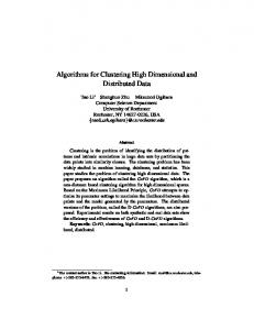
cluster threshold θ from the dataset, aiming to construct a collection of disjoint clusters with high accuracy. With each θi ∈ {0.8, 0.81, ..., 0.99, 1} we apply Algorithm 3 to generate a collection of disjoint clusters and compute its precision using the formula precision(δ, θi , |DB|). The best θ comes from maxθi {precision(δ, θi , |DB|)}. Note that θi begins with 0.8. This value was observed in our experiments. It may vary from application to application. In addition, to obtain clusters with largest possible sizes, one may apply different cluster thresholds: a relatively small one for large cluster cores and a relatively big one for small cluster cores. Again, such cluster thresholds can be observed during the learning process. We performed our experiments on a PC computer with a Pentium 4 2.80GHz CPU and 1GB of RAM. To approximate maximum cluster cores (Algorithm 2), we set maxitr = 10 (i.e. we do 10 times of iteration). In Step 1, different similarity thresholds were tried, with different accuracy results produced as shown in Figure 2. Clearly, δ = 15 is the best for the Mushroom dataset. With this similarity threshold, in Step 2 we applied different cluster thresholds and obtained different accuracy results as shown in Figure 3. We see that the highest accuracy is obtained at θ = 0.88. The sizes of clusters that were produced with δ = 15 and θ = 0.88 are shown in Table 2 (C# stands for the cluster number and the results of ROCK were copied from [10]). Note that our method achieves higher accuracy than ROCK.
Figure 2. Accuracy with varying similarity thresholds. To show that the two thresholds learned via Steps 1 and 2 are the best, we made one more experiment by learning the two parameters together. That is, for each δi ≤ d and θj ∈ {0.8, 0.81, ..., 0.99, 1}, we compute precision(δi , θj , |DB|). If δ and θ selected in Steps 1 and 2 are the best, we expect precision(δ, θ, |DB|) ≈ maxδi ,θj {precision(δj , θj , |DB|)}. Apparently, Figure 4 confirms our expectation. In addition to having high clustering accuracy, our cluster cores-based method can achieve high accuracy when being applied to make classifications. The basic idea is as
Figure 3. Accuracy with varying cluster thresholds given δ = 15.
Figure 4. Accuracy with varying similarity and cluster thresholds.
follows. We first apply Algorithm 3 over a training dataset to learn a similarity threshold δ and generate a collection of disjoint cluster cores with this threshold and θ = 1. Then, we label each cluster core with a class. Next, for each new object o to be classified we count the number Ni of similar objects of o in each cluster core Cir . Finally, we compute i = maxi {Ni /|Cir |} and label o with the class of Cir . We also made experiments for classification on the Mushroom data. The 8,124 objects of the Mushroom dataset have already been divided into a training set (5416 objects) and test set (2,708 objects) on the SGI website (http://www.sgi.com/tech/mlc/db/). The experimental results are shown in Figure 5, where we obtain over 98% of classification accuracy at δ = 15.
6 Conclusions and Future Work We have presented a new clustering approach based on the notion of cluster cores, instead of nearest neighbors. A cluster core represents the core/center of a cluster and thus
using cluster cores to derive clusters achieves high accuracy. Since clusters are not defined in terms of nearest neighbors, our method does not incur the curse of dimensionality and is scalable linearly with the dimensionality of data. Outliers are effectively eliminated by cluster cores, as an outlier would be similar to no or just a very few objects in a cluster core. Although our approach needs three thresholds, α (the minimum size of a cluster core) and δ (the similarity threshold) and θ (the cluster threshold), the last two can well be learned from data. We have shown that our approach outperforms both in efficiency and in accuracy the well-known ROCK algorithm. Like all similarity matrix/graph-based approaches, most of the time of our approach is spent in building a similarity graph. Therefore, as part of future work we are seeking more efficient ways to handle similarity graphs of massive datasets. Moreover, we are going to make detailed comparisons with other closely related approaches such as SNN [6].
ACM SIGMOD Intl. Conf. Management of Data, pp. 73-84, 1998. [10] S. Guha, R. Rastogi and K. Shim, ROCK: A robust clustering algorithm for categorical attributes, in: Proc. ICDM Intl. Conf. on Data Engineering, pp. 512521, 1999. Figure 5. Accuracy of clustering-based classification (Mushroom data).
References [1] J. Abello, P.M. Pardalos and M.G.C. Resende, On maximum cliques problems in very large graphs, in: (J. Abello and J. Vitter, Eds.) DIMACS Series on Discrete Mathematics and Theoretical Computer Science, American Mathematical Society (50): 119-130 (1999). [2] C. C. Aggarwal and P. S. Yu, Finding generalized projected clusters in high dimensional spaces, in: Proc. of ACM SIGMOD Intl. Conf. Management of Data, pp. 70-81, 2000. [3] R. Agrawal, J. Gehrke, D. Gunopolos and P. Raghavan, Automatic subspace clustering of high dimentional data for data mining applications, ACM SIGMOD Intl. Conf. Management of Data, pp. 94-105, 1998. [4] M. R. Anderberg, Cluster Analysis for Applications, Academic Press, New York and London, 1973. [5] M. Ester, H. P. Kriegel, J. Sander and X. Xu, A density-based algorithm for discovering clusters in large spatial databases with noise, in: Proc. 2nd Intl. Conf. Knowledge Discovery and Data Mining, pp. 226-231, 1996.
[11] J. Han and M. Kamber, Data Mining: Concepts and Techniques, Morgan Kaufmann Publishers, 2000. [12] A. Hinneburg, C. C. Aggarwal and D. A. Keim, What is the nearest neighbor in high dimentional spaces? VLDB, pp. 506-515, 2000. [13] A. Hinneburg and D. A. Keim, Optimal gridclustering: towards breaking the curse of dimentionality in high-dimentional clustering? VLDB, pp. 506517, 1999. [14] A. K. Jain and R. C. Dubes, Algorithms for Clustering Data, Prentice-Hall, 1988. [15] A. K. Jain, M. N. Murty and P. J. Flynn, Data clustering: a review, ACM Computing Surveys 31(3): 264323 (1999). [16] R. A. Jarvis and E. A. Patrick, Clustering using a similarity measure based on shared nearest neighbors, IEEE Transactions on Computers C-22(11): 264-323 (1973). [17] G. Karypis, E.-H. Han and V. Kumar, Chameleon: Hierarchical clustering using dynamic modeling, IEEE Computer 32(8): 68-75 (1999). [18] R. T. Ng and J. Han, Efficient and effective clustering methods for spatial data mining, in: Proc. 20th Intl. Conf. Very Large Data Bases, pp. 144-155, 1994. [19] C. M. Procopiuc, M. Jones, P. K. Agarwal and T. M. Murali, A monte carlo algorithm for fast projective clustering, ACM SIGMOD Intl. Conf. Management of Data, pp.418-427, 2002.
[6] L. Ertoz, M. Steinbach and V. Kumar, Finding clusters of different sizes, shapes, and densities in noisy, high dimensional data, in: Proc. 3rd SIAM International Conference on Data Mining San Francisco, CA, USA, 2003
[20] W. Wang, J. Yang and R. Muntz, STING: a statistical information grid approach to spatial aata mining, in: Proc. of the 23rd VLDB Conference, pp. 186-195, 1997.
[7] T.A. Feo and M.G.C. Resende, Greedy randomized adaptive search procedures, J. of Global Optimization (6): 109-133 (1995).
[21] I. H. Witten and E Frank, Data Mining: Practical Machine Learning Tools and Techniques with Java Implementations, Morgan Kaufmann Publishers, 1999.
[8] K. Fukunaga, Introduction to Statistical Pattern Recognition, Academic Press, 1990.
[22] T. Zhang, R. Ramakrishnan and M. Livny, Birch: an efficient data clustering method for very large databases, in: Proc. ACM SIGMOD Intl. Conf. Management of Data, pp.103-114, 1996.
[9] S. Guha, R. Rastogi and K. Shim, CURE: An efficient clustering algorithm for large databases, in: Proc.