Jul 3, 2014 - calculation of the entropy. This can be very well illustrated by the so called. Gibbs paradox. 1.6. The Gibbs paradox. Consider thus the entropy ...
Cluster expansion methods in rigorous statistical mechanics Aldo Procacci July 3, 2014
2
Contents I
Classical Continuous Systems
5
1 Ensembles in Continuous systems 1.1 The Hamiltonian and the equations of motion . 1.2 Gibbsian ensembles . . . . . . . . . . . . . . . 1.3 The Micro-Canonical ensemble . . . . . . . . . 1.4 The entropy is additive. An euristic discussion 1.5 Entropy of the ideal gas . . . . . . . . . . . . . 1.6 The Gibbs paradox . . . . . . . . . . . . . . . 1.7 The Canonical Ensemble . . . . . . . . . . . . 1.8 Canonical Ensemble: Energy fluctuations . . . 1.9 The Grand Canonical Ensemble . . . . . . . . . 1.10 The Thermodynamic limit . . . . . . . . . . . . 1.11 The ideal gas in the Grand Canonical Ensemble
. . . . . . . . . . .
. . . . . . . . . . .
. . . . . . . . . . .
. . . . . . . . . . .
. . . . . . . . . . .
. . . . . . . . . . .
. . . . . . . . . . .
. . . . . . . . . . .
. . . . . . . . . . .
. . . . . . . . . . .
7 7 8 10 12 13 16 18 19 20 22 23
2 The 2.1 2.2 2.3 2.4 2.5 2.6 2.7 2.8 2.9 2.10
Grand Canonical Ensemble Conditions on the potential energy . . . . . Potentials too attractive at short distances . Infrared catastrophe . . . . . . . . . . . . The Ruelle example . . . . . . . . . . . . . Acceptable potentials . . . . . . . . . . . . The infinite volume limit . . . . . . . . . . . Example: finite range potentials . . . . . . Properties the pressure . . . . . . . . . . . . Continuity of the pressure . . . . . . . . . . Analiticity of the pressure . . . . . . . . . .
3 High temperature low density expansion 3.1 The Mayer series . . . . . . . . . . . . . . 3.2 A combinatorial problem . . . . . . . . . . 3.3 The algebraic tree graph identity . . . . . 3.4 The Penrose Identity . . . . . . . . . . . . 3.5 Tree graph stability inequalities . . . . . . 3.6 Tree graph inequalities . . . . . . . . . . . 3.7 The high temperature-low activity phase . 3.8 Examples . . . . . . . . . . . . . . . . . . 3
. . . . . . . .
. . . . . . . . . .
. . . . . . . . . .
. . . . . . . . . .
. . . . . . . . . .
. . . . . . . . . .
. . . . . . . . . .
. . . . . . . . . .
. . . . . . . . . .
. . . . . . . . . .
. . . . . . . . . .
. . . . . . . . . .
. . . . . . . . . .
25 25 28 30 33 35 39 41 44 48 52
. . . . . . . .
. . . . . . . .
. . . . . . . .
. . . . . . . .
. . . . . . . .
. . . . . . . .
. . . . . . . .
. . . . . . . .
. . . . . . . .
. . . . . . . .
. . . . . . . .
. . . . . . . .
57 57 63 65 72 73 75 77 81
4
II
CONTENTS
Lattice systems
83
4 Polymer expansions in the lattice 4.1 Spin systems in a lattice . . . . . . . . . 4.2 Polymer representation of ZΛ (β) . . . . 4.3 The model-independent polymer gas . . 4.4 Mayer series of the abstract polymer gas 4.5 The Koteck´ y-Preiss condition . . . . . . 4.6 An Exercise: counting connected graphs 4.7 The Case of the Lattice gas . . . . . . . 4.8 The bounded spin system case . . . . . 4.9 The unbounded spin system case . . . .
. . . . . . . . .
. . . . . . . . .
. . . . . . . . .
. . . . . . . . .
. . . . . . . . .
. . . . . . . . .
. . . . . . . . .
. . . . . . . . .
. . . . . . . . .
. . . . . . . . .
. . . . . . . . .
. . . . . . . . .
. . . . . . . . .
. . . . . . . . .
85 85 88 90 91 94 97 99 103 105
5 Phase transitions in the Ising model 5.1 Notations . . . . . . . . . . . . . . . 5.2 High temperature expansion . . . . . 5.3 Low temperature expansion . . . . . 5.4 Existence of phase transitions . . . . 5.5 The critical temperature . . . . . . .
. . . . .
. . . . .
. . . . .
. . . . .
. . . . .
. . . . .
. . . . .
. . . . .
. . . . .
. . . . .
. . . . .
. . . . .
. . . . .
. . . . .
107 107 109 115 119 126
. . . . .
. . . . .
Part I
Classical Continuous Systems
5
Chapter 1
Ensembles in Continuous systems
1.1
The Hamiltonian and the equations of motion
Let us consider a system made by a large number N of point particles enclosed in a box Λ ⊂ Rd (we will assume Λ to be cube of size L with volume V ≡ |Λ|) performing a motion according to the laws of classical mechanics. ”Large number of particles” means typically N ≈ 1023 . In this section we will restrict our discussion to systems in three dimensions (i.e. d = 3) composed of identical particles with no internal structure, i.e. just ”point” particles with a given mass m. The position of the ith particle in the box Λ at a given time t is given by a 3 component coordinate vector respect e.g. to some system of orthogonal axis, xi = xi (t) ≡ (xi (t), yi (t), zi (t)). The momenta of the ith particle at time t is also given by a 3-component vector denoted by pi = pi (t) ≡ (pxi (t), pyi (t), pzi (t)). The momenta pi is directly related to the velocity of the particles, i.e. if m is the mass of the particle then i pi = m dx dt . In principle, the laws of mechanics permit to know the evolution of such a system during the time, i.e. these laws should be able to state which positions xi = x(t) and momenta pi = pi (t) the particles in the system will have in the future and had in the past, provided one knows the position of the particles x0i = x(t0 ) and the momenta of p0i = pi (t0 ) at a given time t0 , In fact, the time evolution of such system is described by a real valued function H of particle positions and momentas (hence a function of 6N real variables) called the Hamiltonian. In the case of isolated systems, this function H is assumed to have the form N ∑ p2i H(p1 , p2 , . . . , pN , x1 , . . . , xN ) = + U (x1 , . . . xN ) 2m
(1.1)
i=1
The term
∑N
p2i i=1 2m
is called the (total) kinetic energy of the system, while the 7
8
CHAPTER 1. ENSEMBLES IN CONTINUOUS SYSTEMS
term U (x1 , . . . xN ) is the (total) potential energy. Since we are assuming that particles has to be enclosed in a box Λ we still have to restrict xi ∈ Λ for all i = 1, 2, . . . , N , while no restriction is imposed on pi (i.e. the velocity of particles can be arbitrarily large). Once the of the system is given one could solve the system of 6N differential equations dxi ∂H = dt ∂pi i = 1, 2, . . . , N dpi ∂H = − dt ∂xi
(1.2)
where ∂/∂xi ≡ (∂/∂xi , ∂/∂yi , ∂/∂zi ), and ∂/∂pi ≡ (∂/∂pxi , ∂/∂pyi , ∂/∂pzi ) This is a system of 6N first order differential equations. The solution are 6N functions xi (t), pi (t) if e.g. are known the positions xi (t0 ) and momenta pi (t0 ) at some initial time t = t0 . It is convenient to introduce a 6N -dimensional space ΓN (Λ), called the phase space of the system (with N particles) whose points are determined by the coordinates (q, p) with q = (x1 , . . . , xN ) and p = (p1 , . . . , pN ) (q and p are both 3N vectors!) with the further condition that xi ∈ Λ for all i = 1, 2, . . . , N . A point (q, p) in the phase space of the system is called a microstate of the system. With this notations the evolution of the system during time can be interpreted as the evolution of the a point in the ”plane” q, p (actually a 6N dimension space, the phase space ΓN ). We finally want to remark, by (1.1) that the value of the function H is constant during the time evolution of the system given by (1.2). Namely H(q(t), p(t)) = H(q(0), p(0) (just calculate the total derivative of H respect to the time using equations (1.2)). This constant of motion is called energy of the system and denote with E. Hence E = H(q(0), p(0)) = H(q(t), p(t)). Thus the trajectory of the point q, p in the phase space Γ occurs in the surface H(p, q) = E.
1.2
Gibbsian ensembles
It substantially meaningless to look for the solution of system (1.2). First, there is a technical reason. Namely the system contains an enormous number of equation (≈ 1023 ) which in general are coupled (depending on the structure of U ), so that to find the solution is practically an impossible task. However, even supposing that some very powerful computer would be able to give us the solution, this extremely detailed description (a microscopic description) would not be useful to describe the macroscopic properties of such a system. Macroscopic properties which appear to us as the laws of thermodynamic are due presumably by some mean effects of such large systems and can in general be described in terms of very few parameters, e.g. temperature, volume, pressure, etc.. Hence we have no means and also no desire to know the microscopic state of the system at every instant (i.e. to know the function
1.2.
GIBBSIAN ENSEMBLES
9
(q(t), p(t)). We thus shall adopt a statistical point of view in order to describe the system. We know a priori some macroscopic properties of the system, e.g. an isolated system occupies the volume Λ, has N particles and has a fixed energy E. We further know that macroscopic systems, if not perturbated from the exterior, tends to stay in a situation of macroscopic (or thermodynamic) equilibrium (i.e. a ”static” situation), in which the values of some thermodynamic parameters (e.g. pressure, temperature, etc.) are well defined and fixed. Of course, in a system at the thermodynamic equilibrium, the situation at the microscopic level is desperately far form a static one. Particles in a gas at the equilibrium do in general complicated and crazy motions all the time, nevertheless nothing seems to happens as time goes by at the macroscopic level. So the thermodynamic equilibrium of a system must be the effect os some mean behavior at the microscopic level. This ”static” mean macroscopic behavior of systems composed by a large number of particles must be produced in some way by the microscopic interactions between particle and by the law of mechanics. Adopting the statistical mechanics point of view to describe a macroscopic system at equilibrium means that we renounce to understand how and why a system reach the thermodynamic equilibrium starting from the microscopic level, and we just assume that, at the thermodynamic equilibrium (characterized by some thermodynamic parameters), the system could be find in any microscopic state within a certain suitable set of microstates compatible with the fixed thermodynamic parameters. This is the so called ergodic hypothesis. Namely, all microstates are equivalent. We will also assume that each of this micro-state can occur with a given probability. Of course, in order to have some hope that such a point of view will work, we need to treat really ”macroscopic systems”. So values such N and V must be always though as very large values (i.e. close to ∞). The statistical description of the macroscopic properties of the system at equilibrium (and in particular the law of thermodynamic) is done in two step. 1) Fixing the Gibbsian ensemble (or the space of configurations). We choose a subset Γe of the phase space Γ and we assume that the system can be found in any microstate (q, p) ∈ Γe . This set Γe has to interpreted as the set of all microstates accessible by the system and it is called the Gibbsian ensemble or the space of configurations of the system. Frequently Γe = Γ but, as we will see later, other choices are also possible. So we will simply think not on a single system, but in an infinite number of mental copies of the system Γe ⊂ Γ, one copy for each element of Γe . 2) Fixing the Gibbs measure in the Gibbisan ensemble We choose a function ρ(p, q) in Γe which will represent the probability density in ∫ the Gibbsian ensemble, Namely, ρ(p, q) is a function such that Γe ρ(p, q)dpdq = 1 and dµ(p, q) = ρ(p, q)dpdq represents the probability to find the system in a microstate (or in the configuration) contained in an infinitesimal volume dpdq around the point (p, q) ∈ Γe where dp dq is the usual Lebesgue measure in R6N . The measure µ(p, q) defined in Γe is called the Gibbs measure of the system.
10
CHAPTER 1. ENSEMBLES IN CONTINUOUS SYSTEMS
Once a Gibbsian ensemble and a Gibbs measure are established, one can begin to do statistic in order to describe the macroscopic state of the system. When we look at a macroscopic system described via certain Gibbs ensemble we do not know in which microstate the system is at a given instant. All we know is that its microscopic state must be one of the microstates of the space configuration Γe with probability density given by the Gibbs measure dµ. For example, suppose that f (p, q) is a measurable function respect to the Gibbs measure dµ, such as the energy, the kinetic energy per particle, potential energy etc. Then we can calculate its mean value in the Gibbsian ensemble that we have chosen by the formula: ∫ ⟨f ⟩ = f (p, q)ρ(p, q)dpdq We also recall that the concept of mean relative square fluctuation of f (a.k.a. standard deviation, a.k.a. standard deviation) denoted by σf . This quantity measures how spread is the probability distribution of f (p, q) around its mean value. It is defined as σf
1.3
=
⟨(f − ⟨f ⟩)2 ⟩ ⟨f ⟩2
=
⟨f 2 ⟩ − ⟨f ⟩2 ⟨f ⟩2
(1.3)
The Micro-Canonical ensemble
There are different possible choices for the ensembles, depending on the different macroscopic situation of the system. We start defining the micro-Canonical ensemble which is used to describe perfectly isolated systems. Hence we suppose our system totally isolated from the outside, the N particles are constrained to stay in the box Λ, and they do not exchange energy with the outside, so that the system has a given energy E, occupies a given volume |Λ| and has a fixed number of particles N . Thus, for such a system, we naturally can say that the space of configuration Γmc is the set of points p, q in the phase space with energy between a given value E and E + ∆E (where ∆E can be interpreted as the error we commit measuring the energy E). Γmc = {(p, q) ∈ ΓN (Λ) : E < H(p, q) < E + ∆E,
xi ∈ Λ, ∀i = 1, . . . , N }
The probability measure is chosen in such way that any microstate in the set of configurations above is equally probable, i.e. there is no reason to assign
1.3. THE MICRO-CANONICAL ENSEMBLE
11
different probability to different microstate. This hypothesis is the postulate of equal a priori distribution, which is just a different formulation of the ergodic hypothesis . Hence { [Z(E, Λ, N )]−1 if (q, p) ∈ Γmc ρ(p, q) = 0 otherwise where ∫ Z(E, Λ, N ) = dp dq (1.4) E 0)), and strictly negative around the origin x = 0 (i.e. ∃δ > 0 and b > 0 such that V1bad (|x|) ≤ −b whenever |x| < 2δ). This potential V1bad (|x|) is not stable. In fact if we place N particles in positions x1 , . . . , xN so close one to each other that |xi − xj | < 2δ (i, j = 1, 2, . . . , N ), then U (x1 , . . . , xN ) ≤ −bN (N − 1)/2. First consider a catastrophic situation in which particles collapse in a small region inside Λ. Namely, we calculate, in the Grand Canonical Ensemble with β and µ fixed, the probability to find the system in a micro-state with N = ⟨N ⟩ particles, all located in a small sphere Sδ ⊂ Λ of radius δ (so that they are all at distance less than 2δ). By (2.1) a lower bound for such probability is given by 1 Pbad (N ) = Ξ(β, Λ, λ)
∫
∫ dx1 . . . Sδ
dxN Sδ
λN −βU (x1 ,...,xN ) e ≥ N!
[ ] 1 4 3 N λN +βb N (N −1) 2 ≥ πδ e Ξ(β, Λ, λ) 3 N! Now consider a configuration ”macroscopically correct”, i.e. a micro-state with N particles in positions x1 , . . . xN uniformly spread in all the box Λ, at the density equal to the mean density ρ = ⟨N ⟩/V fixed by the parameters λ and β in the grand canonical ensemble. If the potential V is tempered then it is not difficult to see that for such configurations |U (x1 , . . . , xN )| ≈ CN ρ where ∫ 2C = R3 dx|V (x)|. As a matter of fact, note that, by translational invariance we have that ∑ ∑ |V (|xi − xj |)| = |V (|xj |)| j:j̸=i
j̸=i
Let us now make a partition of the box Λ where particles are confined in small
2.2. POTENTIALS TOO ATTRACTIVE AT SHORT DISTANCES
29
cubes ∆ (with volume |∆|). Hence ∑
∑ ∑
|V (|xj |)| =
∑
|V (|xj |)| ≤
∆ j: xj ∈∆
j: j̸=i
|V (r∆ )|
∑
1
j: xj ∈∆
∆
∑ where ∆ runs over all small cubes and r∆ is the (maximal) distance of the cube ∆ from the origin. Now, since we are assuming that particles are uniformly distributed in Λ and choosing the dimensions of the small cubes sufficiently large in order to still consider this cubes macroscopic, so that the particles in a small cube ∆ are still uniformly distributed with density ρ. Hence ∑ 1 = number of particles in ∆ ≈ ρ|∆| j: xj ∈∆
and
∑
∑
|V (|xi − xj |)| =
j:j̸=i
|V (|xj |)| ≈
∑
|V (r∆ )|ρ∆ ≈
∆
j: j̸=i
∫
∫
≈ ρ
|V (x)|ρdx ≤ ρ
R3
Λ
|V (x)|ρdx
(2.8)
Hence let us consider configurations for which ∑ 1≤i 0 and 3 > ε > 0 and define if |x| ≤ a +∞ (2.9) V2bad (|x|) = −3+ε = −|x| otherwise This potential is a so called hard-core type potential (where the hard core condition is V2bad = + ∞ if |x| ≤ a). It describe a system of interacting hard spheres of radius a. In fact, since V2bad (|x|) is +∞ whenever |x| ≤ r0 , then U (x1 , . . . , xN ) = + ∞ whenever |xi − xj | ≤ a for some i, j, thus the Gibbs factor for such configuration (i.e where some particles are at distances less or equal a) is exp{−βU (x1 , . . . , xN )} = 0 and hence it has zero probability to occur. This means that such system cannot take densities lower than a certain density ρcp called the close-packing density, where particle are as near as possible one to each other compatiblely with the hard core condition. Suppose thus the system in the Grand canonical Ensemble at fixed β and µ, hence at fixed ρ = ⟨N ⟩/V . We choose β and µ in such way that ρ is much smaller that the close-packing density ρcp , i.e. ρ/ρcp ≪ 1. We now compare the probability to find the system in a micro-state near the close-packing situation, e.g. the close-packing configuration dilated of a factor 1 + 2δ (with δ small positive). Each particle can thus move in a small sphere Sδ of radius δ without violating the close-packing configuration. In this set
2.3.
INFRARED CATASTROPHE
31
of configurations the density can vary form the maximum ρcp to a minimum which is at most (1 + 2δ)−3 ρcp . In this case the system does not fill uniformly all the available volume V , it rather occupies a fraction Vcp = N/ρcp of the available volume and leaves a region (with volume V − Vcp = V (ρcp − ρ)/ρ) empty inside Λ. Of course such configurations are non thermodynamics. In these configurations the potential energy U is strongly negative. An upper bound for the value of U for such type of configurations is, by a reasoning similar to that we brought ut to the (2.8): U (x1 , . . . , xN ) ≤ −N [(1 + 2δ)−3 ρcp ]Bε (Vcp ) where, if Λcp denotes the region inside Λ where the N close-packed particles are situated, ∫ Bε (Vcp ) = |x|−3+ε dx x∈Λcp , |x|>a
ε 3
Note that Bε (Vcp ) ∼ Vcp with C constant. Again we bound below the probability to find the system in such bad configurations. ∫ ∫ λN −βU (x1 ,...,xN ) 1 dxN dx1 . . . e ≥ Pbad (N ) = Ξ(β, Λ, λ) Sδ N! Sδ [ ] 1 4 3 N λN +βN (1+2δ)−3 ρcp Bε (Vcp ) ≥ πδ e Ξ(β, Λ, λ) 3 N! An upper bound for ” good” configurations is ∫ ∫ 1 λN −βU (x1 ,...,xN ) Pgood (N ) = e ≤ dx1 . . . dxN Ξ(β, Λ, λ) Λ N! Λ λN +βρN Bε (V ) 1 VN e Ξ(β, Λ, λ) N! Hence the ratio between the probability of bad configurations and good configurations is [ 4 3 ]N +βN (1+2δ)−3 ρ B (V ) cp ε cp πδ e Pbad (N ) ≥ 3 Pgood (N ) V N e+βρN Bε (V ) recalling that V = N/ρ Vcp = N/ρcp ≤
Bε (V ) ∼ CV
ε 3
= CN 3 ρ− 3 ε
ε
we get [
]N
ε
ε
−ε
Bε (Vcp ) ∼ CVcp3 = CN 3 ρcp3 [ ] ε ε 1− ε +βCN 1+ 3 (1+2δ)−3 ρcp 3 −ρ1− 3
Pbad (N ) 4 3 e ≥ πδ ρ Pgood (N ) 3 NN [ ] ε ε 1− Now observe that factor (1 + 2δ)−3 ρcp 3 − ρ1− 3 in the exponential is positive if ρ is suffciently smaller than ρcp and δ sufficiently small. Hence, calling C1 = e
[ ] ε 1− ε +βC (1+2δ)−3 ρcp 3 −ρ1− 3
[ ,
C2 =
4 3 πδ ρ 3
]−1
32
CHAPTER 2. THE GRAND CANONICAL ENSEMBLE
Figure 3. The potential Vbad3 (|x|)
and noting that C1 > 1 we get 1+ ε
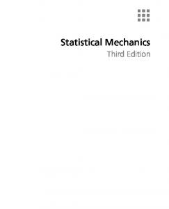
Pbad (N ) C1N 3 ≥ N Pgood (N ) C2 N N It is just a simple exercise to show that this ratio, if C1 > 1 goes to zero as N → ∞ (write e.g. N N = eN ln N ). It is interesting to stress that gravitational interaction behaves at large distances exactly as ∼ |x|−3+ε with ε = 2. Hence we can expect that the matter in the universe do not obey the laws of thermodynamics and in particular it is not distributed as a homogeneous low density gas (an indeed it is really the case!). Consider now a similar case where the pair potential as the same decay as in (2.9), but now is purely repulsive, i.e. suppose if |x| ≤ a +∞ bad V3 = (2.10) = +g|x|−3+ε otherwise This time the bad configurations are those in which particles tend to accumulate at the boundary of Λ in a close packed configuration hence forming a layer. By as argument identical to the one of case 2, supposing ρ < ρcp , one again shows that such configurations are far more probable than ”thermodynamic configurations” (with particles uniformly distributed in Λ). Therefore particles interacting via a potential of type (2.10) will tend to leave the center of the container and accumulate in a layer at the boundary of the container. Again physics gives us an example of potential such as (2.10). That is, the purely repulsive Coulomb potential between charged particles with the same charge. Indeed electrons in excess inside a conductor tends to accumulate at the boundary of the conductor forming layers.
2.4. THE RUELLE EXAMPLE
33
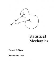
Figure 4. A catastrophic potential. The Ruelle potential
2.4
The Ruelle example
In example 1, V1bad was tempered but not stable. It was a potential strictly negative at the origin. Stability condition is in fact more subtle. Failure of stability can occur also for tempered potential strictly positive in the neighborhood of the origin. We will now consider a very interesting and surprising example of a potential which is strongly positive near the origin, tempered, that nevertheless is a non stable potential. This subtle example, originally due to Ruelle, illustrates very well the intuitive fact that stability condition is there to avoid the collapse of many particles into a bounded region of Rd and it also shows the key role played by the continuum where we have always the possibility to put an arbitrary number of particles in a small region of Rd . Let R > 0 and let δ > 0 11 if |x| < R − δ (2.11) V4bad (x) = −1 if R − 2δ ≤ |x| ≤ R + 2δ 0 otherwise This is clearly a tempered potential (actually it is a finite range potential: particles at distances greater than R + 2δ do not interact at all). But we’ll show that this is a non stable potential by proving that the grand canonical ˜1, . . . , x ˜ n be sites of a partition function diverges for such a potential. Let x face-centered cubic lattice in three dimension with nearest neighborhoods at distance R. We recall that a face-centered cubic lattice is a lattice whose unit cells are cubes, with lattice points at the center of each face of the cube, as well as at the vertices. ˜ n ) = {{i, j} : |˜ ˜ j | = R} the set of nearest neighLet B(˜ x1 , . . . , x xi − x ˜1, . . . , x ˜ n and let Bn = |B(˜ ˜ n )| the cardinality of borhood bonds in x x1 , . . . , x
34
CHAPTER 2. THE GRAND CANONICAL ENSEMBLE
˜1, . . . , x ˜ n are arranged in such way to maximize Bn , this set. Suppose that x hence in a ”close-packed” configuration. We remind that in the face centered ˜1, . . . , x ˜ n to cubic lattice every site has 12 nearest neighborhoods. If we take x be close-packed, then if n is sufficiently large, the number of nearest neighborhoods bond are of the order Bn ∼ 6n. In fact each site is the vertex of 12 nearest neighborhoods bonds, each nearest neighborhood bond is shared between two sites. If n is chosen sufficiently large then it is surely possible to find ˜1, . . . , x ˜ n in such way that a close-packed configuration x Bn >
11 n+ε 2
(2.12)
for some ε > 0. If (2.12) is satisfied, then n ∑ n ∑
˜ j |) = nV (0) + 2Bn V (R) = 11n − 2Bn < −2ε < 0 V (|˜ xi − x
i=1 j = 1
∑ ∑ The function Φ : R6n → R : (y1 , . . . , yn , z1 , . . . , zn ) 7→ ni=1 nj = 1 V (|yi − zj |) ˜n, x ˜1, . . . , x ˜ n ). Moreover, for δ > 0 takes the value −2ε at x ˜ = (˜ x1 , . . . , x chosen to be equal (or smaller) to the one that appears in (2.10) we have that δ ˜1| < , |y1 − x 2
δ ˜n| < , |yn − x 2
...,
implies
n n ∑ ∑
δ ˜1| < , |z1 − x 2
V (|yi − zj |) < −2ε
...
˜n| < |zn − x
δ 2
(2.13)
i=1 j = 1
˜ i | < δ/2} be the open sphere Sδi = {x ∈ R3 : Let now Sδi = {x ∈ R3 : |x − x 3 ˜ i | < δ/2} in R with radius δ/2 and center in x ˜ i and define Λδ = ∪ni = 1 Sδi |x− x (Λδ is of course a subset of R3 ). Let s be a positive integer and define Ms as the following subset of R3sn ˜ i | < δ/2, p = 1, ..., s i = 1, ..., n} Ms = {(x1 , . . . , xsn ) ∈ R3sn : |x(i−1)s+p − x Namely, (x1 , . . . , xsn ) ∈ Ms means that the sn-uple (x1 , . . . , xsn ) is such that the first s variables x1 , . . . , xs of the sn-uple are all inside the sphere Sδ1 , the variables xs+1 , . . . , x2s are all inside the sphere Sδ2 , the variables x2s+1 , . . . , x3s are all inside the sphere Sδ3 , and so on until the last s variables of the sn-uple, which are x(n−1)s+1 , . . . , xsn , and are all inside the sphere Sδn . Now, if (x1 , . . . , xsn ) ∈ Ms , then, sn sn ∑ 1 ∑ ∑ U (x1 , ..., xsn ) = V (|xi − xj |) = V (|xi − xj |) − snV (0) = 2 1≤i0
36
CHAPTER 2. THE GRAND CANONICAL ENSEMBLE
Figure 5. A Lennard-Jones potential
2 - Positive type potentials: ∫ V˜ (k)eik·x d3 k,
V (x) =
V˜ (k) ≥ 0
3 - Lennard-Jones Potentials: V (x) ≥
C1 for x ≤ a, |x|3+ε
|V (x)| ≤
C2 for x > a |x|3+ε
We remark that potentials with hard core (V (x) = + ∞ if |x| ≤ a) can be included in case 3 or in case 1. Let us show that a potential of type 1 is acceptable. It is tempered (i.e. it satisfies (2.7)) by definition and it is stable, since from V (x) ≥ 0 we get U (x1 , . . . , xn ) ≥ 0
∀n, x1 , . . . , xn
hence (2.6) is verified with B = 0. Let us show now that a potential of type 2 is acceptable. We denote by 0 the null vector in R3 . A positive type potential V is stable because ∑
U (x1 , . . . , xn ) =
V (xi − xj ) =
1≤i 0. Therefore, finally Therefore, finally, iterating this formula we get x3
U (x1 , . . . , xn ) ≥ −Cn Case 2) rmin ≥ a/2. In this case we write 1∑ 2 n
U (x1 , . . . , xn ) =
∑
V (xi − xj )
i=1 j∈{1,2,...,n}: j̸=i
∑ and we will get an estimate j∈{1,2,...,n}, j̸=i V (xi − xj ). First note that, since all particles are at distances ≥ a/2 we can bound ∑ j∈{1,2,...,n} j̸=i
V (xi − xj ) ≥ −
∑ j∈{1,2,...,n} j̸=i
C2 |xi − xj |3+ε
We then proceed analogously as before. √ This time, for fixed i, we can draw around each xj a cube Qj with side a/ 48 (such that the maximal diagonal of Qj is a/4) with xj being the vertex farthest away from xi . Since any two points among x1 , . . . , xn are at mutual distances ≥ a/2 the cubes so constructed do not overlap. Moreover if we consider the open sphere Si = {x ∈ R3 : |x − xi | < a4 } and denote by Sic its complementar in R3 , then by construction ∪j̸=i Qj ⊂ Sic . In other words all cubes Qj lay outside the open sphere with center xi and radius a/4. Furthermore we have √ ∫ 1 ( 48)3 1 ≤ d3 x 3+ε 3 3+ε |xi − xj | a |x − x| i Qj
2.6. THE INFINITE VOLUME LIMIT
39
recall in fact that the cube Qj is chosen in such way that |x − xi | ≤ |xi − xj | for all x ∈ Qj . Therefore √ ( 48)3 V (xi − xj ) ≥ − C2 a3 j∈{1,2,...,n} ∑
∑
j̸=i
j∈{1,2,...,n} j̸=i
∫ Qj
1 d3 x ≥ |xi − x|3+ε
√ ∫ ( 48)3 1 d3 x ≥ ≥ − C2 3 3+ε a |x − x| i ∪j Qj √ 3∫ ( 48) 1 ¯a ≥ − C2 d3 x ≥ − K 3 3+ε a |x|≥a/4 |xi − x| where ¯a K Hence
√ ∫ ( 48)3 1 = C2 d3 x 3+ε a3 |x − x| i |x|≥a/4 ∑
¯a V (xi − xj ) ≥ − K
(2.14)
j∈{1,2,...,n} j̸=i, |xi −xj | > a
and U (x1 , . . . , xn ) ≥ −
2.6
¯a K n 2
The infinite volume limit
We will now start to consider the problem of the existence of the thermodynamic limit for the pressure of a system of particles in the grand canonical ensemble interacting via a pair potential stable and tempered. The mathematical problem is to show the existence of the infinite volume pressure defined as βp(β, λ) =
1 ln Ξ(Λ, β, λ) Λ→∞ V (Λ) lim
(2.15)
where V (Λ) is the volume of Λ. First of all we need to give a mathematical meaning to the notation Λ → ∞ in (2.15). We know that Λ is a finite region of R3 and it can tend to infinity (namely its volume tends to infinity) in various way. For instance Λ could be a cylinder of fixed base A and height h and we could let h → ∞. I.e. like a cigar with increasing length. It is obvious that such a system (particularly if A is very small) is not expected to have a thermodynamic behavior even if h → ∞. Thus Λ → ∞ cannot simply be V (Λ) → ∞, since we want to exclude cases like ”the cigar” which is not a scandalous if they do not yield thermodynamic behavior. We need thus that Λ → ∞ roughly in such way that Λ is big in every direction, e.g. a sphere of increasing radius, a cube of increasing size etc. We will review the following definitions
40
CHAPTER 2. THE GRAND CANONICAL ENSEMBLE
Figure 6. A box Λ going to infinity in a ”non-thermodynamic” way
Definition 2.1 Λ is said to go to infinity in the sense of Van Hove if the following occurs. Cover Λ with small cubes of size a and let N+ (Λ, a) the number of cubes with non void intersection with Λ and N− (Λ, a) the number of cubes strictly included in Λ. Then Λ → ∞ in the sense of Van Hove if
N− (Λ, a) → ∞,
and
N+ (Λ, a) →1 N− (Λ, a)
∀a
See figure 7. As an example, it is easy to show that if Λ → ∞ as in the case of the “cigar” seen before, then Λ is not tending to infinity in the sense of Van Hove. Consider thus, for sake of simplicity in the plane, a rectangle R with sizes l fixed and t variable and going to infinity. Let consider squares of size a to cover the rectangle. Then N− (R, a) = thus
l t , aa
N+ (R, a) =
l t t l +2 +2 aa a a
l N− (R, a) = ̸= 1 t→∞ N+ (R, a) l+2 lim
√ On the other hand, let us check that a rectangle of sizes ( t, t) and tends to infinity, as t → ∞, in the sense of Van Hove. As a matter of fact √ √ √ tt tt t t N− (R, a) = , N+ (R, a) = +2 +2 a a a a a a thus
√ N− (R, a) t t √ = 1 lim = lim √ t→∞ N+ (R, a) t→∞ t t + 2t + 2 t
For a given Λ let V (Λ) denote its volume, let Vh (Λ) denotes the volume of the set of points at distance h from the boundary of Λ and let d(Λ) denote the diameter of Λ (i.e. d(Λ) = supx,y∈Λ {|x − y|}) . Definition 2.2 We say that Λ tends to infinity in the sense of Fischer if V (Λ) → ∞ and it exists a positive function π(α) such that limα→0 π(α) = 0 and for a sufficiently small e for all Λ Vαd(Λ) (Λ) ≤ π(α) V (Λ)
2.7. EXAMPLE: FINITE RANGE POTENTIALS
41
Figure 7. A set Λ with N+ = 44 and N− = 20
A rectangle R of sizes f (t), t such that limt→∞ in the sense of Fischer. As a matter of fact
f (t) t
= 0 does not go to infinity
d(R) = [t2 + f 2 (t)]1/2 Vαd(R) (R) = 2α[t2 + f 2 (t)]1/2 [t − 2α[t2 + f 2 (t)]1/2 + f (t)] Vαd(R) (R) 2α[t2 + f 2 (t)]1/2 [t − 2α[t2 + f 2 (t)]1/2 + f (t)] = V (R) tf (t) √ √ 2 2 2αt2 1 + f t2(t) [1 − 2α 1 + f t2(t) + f (t) t ] √ = t t For any fixed α the quantity above can be make large at will, as t → ∞. Thus it is not possible to find any π(α) such that Vαd(R) (R)/V (R) ≤ π(α) for all R (i.e. for all t). On the other hand, the square S of size (t, t) goes to infinity in the sense of Fischer √ √ √ d(S) = 2t, Vαd(R) (R) = 4α 2t[t − α 2t] √ √ √ √ √ Vαd(R) (R) 4α 2 t[t − α 2t] = = 4α 2[1 − α 2] ≤ 4α 2 2 V (R) t √ Hence one can choose π(α) = 4α 2.
2.7
Example: finite range potentials
We will prove in this section the existence of the thermodynamic limit for the function βp(β, λ) defined in (2.15), but we will not treat the general case, namely particles interacting via a pair potential stable and tempered and Λ going to infinity as e.g. Van Hove. We will rather give our proof in a simpler case. Namely, we will assume that particles interact through a stable and tempered
42
CHAPTER 2. THE GRAND CANONICAL ENSEMBLE
˜ n+1 and the cubes Λn , Λ ˜n Figure 8. The cubes Λn+1 , Λ
pair potential V (x) with the further property that it exists r¯ > 0 such that V (x) ≤ 0 if |x| ≥ r¯, i.e. the potential is negative for distances greater than r¯. In order to make things even simpler we will also suppose that Λ is a cube of size L and Λ → ∞ ⇔ L → ∞. We now choose two particular sequences ˜ 1, Λ ˜ 2, . . . , Λ ˜ n , . . . of cubes. Let Λ1 be a cube of size L1 Λ1 , Λ2 , . . . , Λn , . . . and Λ ˜ 1 is a new cube of size L ˜ 1 = L1 + r¯ which consists of with volume V1 while Λ r¯ ˜ Λ1 plus a frame of thickness 2 . We denote V1 it volume (of course V˜1 > V1 ) Λ2 is a cube of size L2 = 2L1 + r¯, thus in Λ2 we can arrange 23 = 8 cubes Λ1 with with frames of thickness r¯/2 in such way that any point in a given cube Λ1 inside Λ2 is at distance greater that r¯ from any point in any other cube Λ1 ˜ 2 is a cube of size 2L ˜ 1 , i.e. is the cube Λ2 plus a frame inside Λ2 . Of course Λ of thickness r¯. See figure 8. ˜ n+1 is a cube of size In general Λn+1 is a cube of size Ln+1 = 2Ln + r¯ and Λ ˜ n+1 = 2L ˜ n = 2Ln + 2¯ L r Note that Vn+1 > 8Vn and V˜n+1 = 8Vn and also ˜ limn→∞ Vn /Vn = 1. We will now show that the sequence of functions Pn (λ, β) = βpn (β, λ) =
1 ln Ξ(β, λ, Λn ) V (Λn )
(2.16)
tends to a limit. Define the sequence P˜n =
1 ln Ξ(β, λ, Λn ) ˜ V (Λn )
(2.17)
We will first show that this sequence converges to a limit. Consider the sequence Ξn = Ξ(β, λ, Λn ). We have ∫ ∞ ∑ λN Ξn+1 = d3 x1 . . . d3 xN e−βU (x1 ,...,xN ) N ! ΛN n+1 N = 0
2.7. EXAMPLE: FINITE RANGE POTENTIALS
43
We now think Λn+1 as the union of 8 cubes Λjn (j = 1, 2, . . . , 8) plus the frames. Obviously if we calculate Ξn+1 eliminating the configurations in which particles can stay in the frames we are underestimating Ξn+1 . I.e. Ξn+1
∫ ∞ ∑ λN > d3 x1 . . . d3 xN e−βU (x1 ,...,xN ) N ! ∪j Λjn N = 0
Thus the N particles are arranged in such way that N1 are in the box Λ1n , N2 are in the box Λ2n ..., and Nn8 are in the box Λ8n . Thus we can rename coordinates x1 , . . . , xN as x11 , . . . x1N1 , . . . , x81 , . . . x8N8 . The interaction between particles in different boxes is surely non positive (since they are at distances greater or equal to r¯) then U (x1 , . . . , xN ) = U (x11 , . . . x1N1 , . . . , x81 , . . . x8N8 ) ≤ ≤ U (x11 , . . . x1N1 ) + . . . + U (x81 . . . x8N8 ) and hence e−βU (x1 ,...,xN ) ≥ e
[ ] −β U (x11 ,...x1N ) + ... + U (x81 ...x8N ) 1
8
The number of ways in which such arrangement can occur is ( )( ) ( ) N N − N1 N − N1 − N2 − . . . − N7 N! ... = N1 N2 N8 N1 ! . . . N8 ! Hence ∑
Ξn+1 >
N1 ,...,N8
∫ ···
N! λN1 +...+N8 N! N1 ! . . . N8 !
∫
Λ8n
d3 x81 . . .
Λ8n
d3 x8N8 e
∫ Λ1n
∫ d3 x11 . . .
−βU (x11 ,...,x1N ) −βU (x21 ,...,x2N ) 1
e
2
Λ1n
...e
d3 x1N1 · · ·
−βU (x81 ,...,x8N ) 8
=
= (Ξn )8 So we have shown that Ξn+1 > (Ξn )8 Hence, since f (x) = ln x is a monotonic increasing function, we also get ln Ξn+1 > ln(Ξn )8 and
1 1 1 ln Ξn+1 > ln(Ξn )8 = ln Ξn ˜ ˜ ˜ V (Λn+1 ) V (Λn+1 ) V (Λn )
So the sequence P˜n is monotonic increasing with n. On the other hand by stability we have that. Ξn =
∫ ∞ ∑ λN d3 x1 . . . d3 xN e−βU (x1 ,...,xN ) ≤ N ! ΛN n
N = 0
44
CHAPTER 2. THE GRAND CANONICAL ENSEMBLE ≤
∫ ∞ ∑ λN d3 x1 . . . d3 xN e+βN = exp λVn eβB N ! ΛN n
N = 0
therefore, ln Ξn ≤ λVn eβB and
1 1 ln Ξn ≤ λVn eβB ≤ λeβB ˜ ˜ Vn Vn This means that the sequence P˜n is monotonic increasing and bounded above. Hence limn→∞ P˜n = P exists. But now P˜n =
Pn = whence lim Pn =
n→∞
V˜n ˜ 1 Ξn = Pn Vn Vn
V˜n ˜ Pn = n→∞ Vn lim
V˜n lim P˜n = P n→∞ Vn n→∞ lim
Therefore we show the existence of the thermodynamic limit for a class of systems interacting via a potential which, beyond being tempered and stable, has the further property to be non positive for |x| ≥ r¯, when Λ goes to infinity along the sequence of cubes Λn . It is not difficult from here to show that the existence of such limit implies also that the limits exists if Λ is a cube which goes at infinity in sense homothetic (i.e. the size Λ → ∞). Actually, the existence of limits can be proved for much more general cases, see e.g. theorem 3.3.12 in [11]
2.8
Properties the pressure
Let us now show some general properties of the limit for the pressure βp(β, λ) in (2.15). The pressure p(β, λ) is a function of two variables λ and β which are the two independent thermodynamic parameters describing the macroscopic equilibrium state in the Grand canonical ensamble. We are interested to study the function βp(β, λ) only for the ”physically” admissible values of λ and β. These physical values are: λ real number in the interval∈ (0, +∞) and β real number in the interval ∈ (0, +∞) (recall definition (1.31)). The Grand canonical partition function Ξ(β, Λ, λ) defined in (2.2) where we are supposing of course that U (x1 , . . . , xN ) is derived from a stable and tempered pair potential has the following structure
Ξ(λ, b, Λ) = 1 + Z1 (Λ, β)λ + =
Z2 (Λ, β) 2 Z3 (Λ, β) 3 λ + λ + ... = 2! 3!
∞ ∑ ZN (Λ, β) N λ N!
N = 0
I.e. is a power series in λ with convergence radius R = ∞ (this is true for any Λ such that V (Λ) < ∞), i.e., Ξ(λ, β, Λ) is analytic as a function of λ in the
2.8. PROPERTIES THE PRESSURE
45
whole complex plane. Hence a fortiori Ξ(λ, b, Λ) is analytic for all λ ∈ (0, +∞). This is true for all Λ such that V (Λ) < ∞ The coefficients ZN (Λ, β) are explicitly given by ∫ ∫ ZN (Λ, β) = dx1 . . . dxN e−βU (x1 ,...,xN ) (2.18) Λ
Λ
They are clearly all positive numbers and due to stability (recall proposition 1) they admit the upper bound ZN (Λ, β) ≤ [V (Λ)]n eN Bβ . Moreover as function of β the coefficients CN (Λ, β) are analytic in β in the whole complex plane and hence a fortiori for all β ∈ (0, ∞). So, Ξ(λ, β, Λ), for all Λ such that V (Λ) < ∞, and for all λ ∈ (0, +∞) is also analytic as a function of β in the whole complex plane. Hence a fortiori Ξ(λ, β, Λ) is analytic for all β ∈ (0, +∞). Now the function ln Ξ(λ, β, Λ) has no reason to continue analytic in λ and β in the whole complex plane, but it is indeed analytic in λ for any λ ∈ (0, +∞) and it is analytic in β for all β ∈ (0, +∞). This is due to the fact that coefficients Cn (Λ, β) are positive numbers. Hence Ξ(λ, b, Λ) has no zeroes in the intervals λ ∈ (0, +∞) and β ∈ (0, +∞). This means that its logarithm is analytic for such intervals. In conclusion we can state that the function βpΛ =
1 ln Ξ(λ, β, Λ) = fΛ (λ, β) V (Λ)
(2.19)
is analytic in λ for all λ ∈ (0, +∞) and it is also analytic in β for all β ∈ (0, +∞), whenever on choose a volume Λ such that V (Λ) < ∞. This fact of course does not imply that also in the limit Λ → ∞ the function βp(λ, β) will stay analytic in the whole physical intervals λ ∈ (0, +∞) and β ∈ (0, +∞). Let us now list some properties of the function βpΛ (β, λ) defined by (2.19). Property 0a. fΛ (λ, β) defined in (2.19) is continuous as a function of λ and all its derivatives are continue as functions of λ in the whole interval λ ∈ (0, +∞) and for all β ∈ (0, +∞) and for all Λ such that V (Λ) < ∞. Property 0b. fΛ (λ, β) defined in (2.19) is continuous as a function of β and all its derivatives are continue as functions of β in the whole interval β ∈ (0, +∞) and for all λ ∈ (0, +∞) and for all Λ such that V (Λ) < ∞. This properties follow trivially from the fact that βpΛ (β, λ) is analytic in λ and β when they vary in the interval (0, +∞). Property 1. fΛ (λ, β) defined in (2.19) is monotonic increasing as a function of λ in the interval λ ∈ (0, +∞), for all β ∈ (0, +∞) and for all Λ such that V (Λ) < ∞ In order to show the property 1 it is sufficient to show that
∂fΛ (λ,β) ∂λ
∂fΛ (λ, β) 1 ∂Ξ(λ, b, Λ)/∂λ ρΛ (λ, β) = = ∂λ V (Λ) Ξ(λ, b, Λ) λ
≥ 0. But (2.20)
46
CHAPTER 2. THE GRAND CANONICAL ENSEMBLE
where ρ(λ, β) = ⟨N ⟩/V (Λ) is the density and ⟨N ⟩Λ (λ, β) is the mean number of particles in the grand canonical ensemble at fixed values of λ, β and Λ. Explicitly ⟨N ⟩Λ (λ, β) is given by ⟨N ⟩Λ (λ, β) =
∑∞
λN N =0 N ! N ZN (Λ, β) ∑ ∞ λN N =0 N ! ZN (Λ, β)
Hence, since ⟨N ⟩ is surely a positive number for λ > 0, we get ∂fΛ (λ, β) >0 ∂λ Property 2. fΛ (λ, β) defined in (2.19) is convex as a function of ln λ in the interval λ ∈ (0, +∞), for all β ∈ (0, +∞) and for all Λ such that V (Λ) < ∞. Moreover the finite volume density ρΛ (λ, β) = ∂(ln∂ λ) fΛ (λ, β) is a monotonic increasing function of ln λ. As a matter of fact ∂ ∂ fΛ (λ, β) = λ fΛ (λ, β) = ρΛ (λ, β) ∂(ln λ) ∂λ Last line follows by (2.20). Moreover ∂2 λ ∂ ∂ ⟨N ⟩ = fΛ (λ, β) = λ ρΛ (λ, β) = ∂(ln λ)2 ∂λ V (Λ) ∂λ ] [∑ ∞ λN ) N Z (Λ, β) 1 ( 2 λ ∂ N N = 0 N! = ⟨N ⟩ − ⟨N ⟩2 = = ∑∞ N λ V (Λ) ∂λ V (Λ) ZN (Λ, β) N = 0 N!
=
⟨(N − ⟨N ⟩)2 ⟩ V (Λ)
where ⟨N ⟩ = 2
(2.21)
∑∞
λN 2 N =0 N ! N ZN (Λ, β) ∑ ∞ λN N =0 N ! ZN (Λ, β)
thus, since the factor ⟨(N − ⟨N ⟩)2 ⟩ is always positive we get ∂2 ∂ fΛ (λ, β) = ρΛ (λ, β) > 0 ∂(ln λ)2 ∂(ln λ) This prove that fΛ (λ, β) is convex in the variable ln λ and that ρΛ (λ, β) is monotonic increasing in ln λ. Property 3. fΛ (λ, β) defined in (2.19) is convex as a function of β in the interval β ∈ (0, +∞), for all λ ∈ (0, +∞) and for all Λ such that V (Λ) < ∞. As a matter of fact ∂ 1 ∂ ⟨−U ⟩ fΛ (λ, β) = ln Ξ(Λ, β, λ) = ∂β V (Λ) ∂β V
2.8. PROPERTIES THE PRESSURE
47
where ∫ ∫ ∞ ∑ 1 λN ⟨−U ⟩ = dx1 . . . dxN [−U (x1 , . . . , xN )]e−βU (x1 ,...,xN ) Ξ(Λ, β, λ) N! Λ Λ N = 0
Deriving one more time respect to β ⟨U 2 ⟩ − ⟨U ⟩2 ∂2 f (λ, β) = Λ ∂β 2 V (Λ) where ∫ ∫ ∞ ∑ 1 λN ⟨U ⟩ = dx1 . . . dxN [U (x1 , . . . , xN )]2 e−βU (x1 ,...,xN ) Ξ(Λ, β, λ) N! Λ Λ 2
N = 0
and since ⟨U 2 ⟩ − ⟨U ⟩2 = ⟨(U − ⟨U ⟩)2 ⟩ ≥ 0 we obtain ∂2 fΛ (λ, β) ≥ 0 ∂β 2 and fΛ (λ, β) is a convex function of β for all Λ such that V (Λ) is finite. Property 4. βp(λ, β) = f (λ, β) = limΛ→∞ βpΛ (β, λ) = limΛ→∞ fΛ (λ, β) is convex and hence continuous as a function of β and λ in the interval β, λ ∈ (0, +∞). This property which is a very important property about the pressure in the thermodynamic limit follows trivially by the fact that the limit of a converging sequence of convex functions is also a convex function and that any convex function defined in an open set is continuous in the same open set. Property 5. It is possible to express, for any Λ finite, the pressure pΛ as a function of ρΛ and β, i.e. pΛ = gΛ (ρΛ , β) moreover the function gΛ (ρΛ , β) is monotonic increasing as a function of ρΛ . The finite volume density is ρΛ = ρΛ (λ, β) = ρΛ (eln λ , β) = FΛ (ln λ, β) Since, by property 3 the function FΛ (x, β) is strictly increasing as a function of x for any Λ finite and any β ∈ (0, +∞), then it admit, as function of x, an inverse, say x = GΛ (ρΛ , β). Hence ln λ = GΛ (ρΛ , β),
λ = eGΛ (ρΛ ,β)
Thus the function g(ρΛ , β) can be indeed constructed and is given explicitly by pΛ = gΛ (ρΛ , λ) =
1 fΛ (eGΛ (ρΛ ,β) , β) β
48
CHAPTER 2. THE GRAND CANONICAL ENSEMBLE
It is now easy to check that this function is monotonic increasing. As a matter of fact ∂ 1 ∂ 1 ∂(ln λ) ∂ pΛ = (βpΛ ) = (βpΛ ) = ∂ρΛ β ∂ρΛ β ∂ρΛ ∂(ln λ) [ ] [ ] 1 ∂ρΛ −1 1 ∂ρΛ −1 = ρΛ = ρΛ λ β ∂(ln λ) β ∂λ recalling now that ρL = ⟨N ⟩/V (Λ) and (2.21) we obtain [ ] ∂ 1 ∂ρΛ −1 1 ⟨N ⟩ p Λ = ρΛ λ = 2 ∂ρΛ β ∂λ β ⟨N ⟩ − ⟨N ⟩2
(2.22)
Formula (2.22) shows that (∂/∂ρΛ )pΛ is always positive. Actually (2.22) tells us also that the value of (∂/∂ρΛ )pΛ is ⟨N ⟩(⟨N 2 ⟩ − ⟨N ⟩2 )−1 . thus if we are able to prove that ⟨N ⟩(⟨N 2 ⟩ − ⟨N ⟩2 )−1 stay bounded away from +∞ for any Λ we can conclude that p(ρ, β) = limΛ→∞ πL (ρΛ β) is continuous a function of the density ρ = limΛ→∞ ρL . Property 6. p = g(ρ, β) is monotonic increasing as a function of ρ (hence monotonic decreasing as a function of ρ−1 ) The monotonicity follows trivially from that fact that pΛ (ρΛ , β) is monotonic increasing for any Λ. Note now that 1 ⟨N ⟩ ∂ pΛ = = CΛ ≥ 0 2 ∂ρΛ β ⟨N ⟩ − ⟨N ⟩2 CΛ is a constant in general depending on Λ.
2.9
(2.23)
Continuity of the pressure
Experimentally the pressure is not only decreasing as a function of ρ−1 but it appears furthermore to have no (jump) discontinuities. A general proof of this fact is still lacking. It has been proven that under suitable conditions on the potential (super-stability) the pressure is indeed continuous as a function of the density (see e.g. Ruelle Comm. Math. Phys. vol. 18, 127-159 (1970)). We prove here this fact in a much simpler case, namely we assume that the pair potential is either hard core, or non negative (i.e. purely repulsive). Our strategy will consist in proving that the constant CΛ in equation (2.23) is bounded uniformly in Λ. This will allow us to conclude that pΛ (ρΛ , β) has a bounded derivative in ρΛ uniformly in Λ, so the limit p(ρ, β) = limΛ→∞ pΛ (ρΛ , β), cannot have vertical jumps as a function of ρ, i.e. p(ρ, β) is continuous as a function of the density. Let us thus prove that ⟨N ⟩ ≤C (2.24) 2 ⟨N ⟩ − ⟨N ⟩2 assuming that the pair potential between particles is hard core or purely repulsive.
2.9. CONTINUITY OF THE PRESSURE
49
Theorem 2.1 Let V be a tempered and stable pair potential. If V is either positive (V ≥ 0) or such that ∃a : V (x) = + ∞ whenever |x| ≤ a (i.e. hard core). Then ⟨N ⟩ ≤ (1 + Dλ) 2 ⟨N ⟩ − ⟨N ⟩2 where D is uniform in Λ. Proof. We will use the following short notations XN = x1 , . . . , xN ,
dXN = dx1 . . . dxN ,
U (XN ) = U (x1 , . . . , xN ), ∫ dx1 . . .
dxN e
Λ
V (xj − x)
j = 1
∫
ZN = ZN (Λ, β) =
N ∑
W (x, XN ) =
∫
−βU (x1 ,...,xN )
dXN e−βU (XN )
= ΛN
Λ
The partition function Ξ(λ, Λ, β) (denoted shortly by Ξ) is thus rewritten ∞ ∑ λN ZN N!
Ξ =
(2.25)
N = 0
With these definitions we have, [∫ ]2 ∫ 2 −βU (XN ) −βW (x,XN ) ZN +1 = dXN e dxe
=
ΛN
[∫ =
dXN e
− β2 U (XN )
ΛN
[∫
∫ dxe
− β2 U (XN ) −βW (x,XN )
e
]2 =
]2 dXN F (XN )G(XN )
= ΛN
where
∫
β
F (XN ) = e− 2 U (XN )
G(XN ) =
Using Schwartz inequality we get [∫ ]2 ∫ dXN F (XN )G(XN ) ≤ ΛN
thus ≤
∫ dXN F 2 (XN )
ΛN
∫
2 ZN +1
∫
dXN e ∫
= Zn ΛN
dXN dxdye−βU (XN ) e−βW (x,XN ) e−βW (y,XN ) =
ΛN
∫ dXN
∫
( ) dye−βU (XN ,x,y) e+βV (x−y) − 1 + 1 =
dx
∫
Λ
= ZN ZN +2 + ZN
Λ
∫
∫
dXN ΛN
dXN G2 (XN ) ΛN
∫
−βU (XN )
ΛN
β
dxe− 2 U (XN ) e−βW (x,XN )
dx Λ
Λ
( ) dye−βU (XN ,x,y) e+βV (x−y) − 1 =
50
CHAPTER 2. THE GRAND CANONICAL ENSEMBLE ∫
∫
= ZN ZN +2 + ZN
∫
dXN ΛN
dxe
−βU (XN ,x)
Λ
( ) dye−βW (XN ,y) 1 − e−βV (x−y)
Λ
Now, since we are assuming V (x) hard core or positive we have { = 1 if V ≥ 0 e−βW (XN ,y) ≤ B(β) = = eβB if V has an hard core a where B is a constant ∝ a−3 (see equation (2.14)). Thus ∫ ∫ ∫ ( ) 2 −βU (XN ,x) ZN +1 ≤ ZN ZN +2 + B(β)ZN dXN dxe dy 1 − e−βV (x−y) ≤ ΛN
Λ
Λ
∫
( ) dy |1 − e−βV (x−y) |
≤ ZN ZN +2 + C(β)ZN ZN +1 Λ
Note now that in the case in which V is positive or have hard core, and also recalling that V must also be tempered, we have ∫ ( ) ∫ −βV (x−y) dy |1 − e | ≤ dx|1 − e−βV (x) | ≤ C(β) < +∞ R3
Λ
and calling D(β) = B(β)C(β) we get finally 2 ZN +1 ≤ ZN ZN +2 + D(β)ZN ZN +1 ⇐⇒
2 ZN +1 ≤ ZN +2 + ZN +1 D(β) (2.26) ZN
Now consider ( 2
(⟨N ⟩[1 + λD(β)])
=
)2 ∞ ∑ λN ZN N [1 + λD(β)] = N! Ξ
N = 0
[ ])2 ∞ ∑ λN ZN λN +1 ZN +1 = + N λD(β) = N! Ξ λN ZN N = 0 ( ∞ ]) 2 ∑ λN ZN [ λ ZN +1 = + N λD(β) N! Ξ ZN (
N = 0
where in the last line we have used ∞ ∑ λN N ZN = N!
N = 0
and by definition (2.25)
∞ ∑ λN +1 ZN +1 N!
N = 0
∞ ∑ λN ZN = 1 N! Ξ
N = 0
Now (
( ∞ )2 [ ])2 ∞ ∑ ∑ λN ZN λZN +1 + N λD(β) = FN · GN N! Ξ ZN
N = 0
N = 0
2.9. CONTINUITY OF THE PRESSURE
51
where ( FN =
λN ZN N! Ξ
)1/2
( GN =
λN ZN N! Ξ
)1/2 [
λZN +1 + N λD(β) ZN
]
using thus again Schwartz inequality we get (
∞ ∑
)2 FN · GN
N = 0
≤(
∞ ∑
N = 0
FN2 )(
∞ ∑
G2N ) =
N = 0
)[ ]2 ∞ ( N ∑ λ ZN ZN +1 = 1× λ + N λD(β) = N! Ξ ZN N = 0
=
]2 )[ ∞ ( N 2 ∑ Z λ 1 λ2 N +1 + 2N λ2 D(β)ZN +1 + ZN N 2 λ2 D2 (β) N! Ξ ZN
N = 0
hence using also (2.26) ) [ ∞ ( N ∑ 1 λ λ2 ZN +2 + (⟨N ⟩[1 + λD(β)])2 ≤ N! Ξ N = 0
]2 + ZN +1 D(β) + 2N D(β)ZN +1 + ZN N 2 D2 (β) Now observe that ) ∞ ( N ∑ λ 1 λ2 ZN +2 = ⟨N (N − 1)⟩ N! Ξ
N = 0
) ∞ ( N ∑ λ 1 λ2 ZN +1 D(β) = λD(β)⟨N ⟩ N! Ξ
N = 0
(
∞ ∑ N = 0
λN 1 N! Ξ
) 2N λ2 D(β)ZN +1 = 2D(β)λ⟨N (N − 1)⟩
) ∞ ( N ∑ λ 1 ZN N 2 λ2 D2 (β) = D2 (β)λ2 ⟨N 2 ⟩ N! Ξ
N = 0
thus (⟨N ⟩[1 + λD(β)])2 ≤ ≤ ⟨N (N − 1)⟩ + λD(β)⟨N ⟩ + 2D(β)λ⟨N (N − 1)⟩ + D2 (β)λ2 ⟨N 2 ⟩ =
= ⟨N 2 ⟩ − ⟨N ⟩ + λD(β)⟨N ⟩ + 2D(β)λ(⟨N 2 ⟩ − ⟨N ⟩) + D2 (β)λ2 ⟨N 2 ⟩ = = ⟨N 2 ⟩(1 + D(β)λ)2 − ⟨N ⟩(1 + λD(β))
52
CHAPTER 2. THE GRAND CANONICAL ENSEMBLE
Thus we are arrived at the inequality ⟨N ⟩2 [1 + λD(β)]2 ≤ ⟨N 2 ⟩(1 + D(β)λ)2 − ⟨N ⟩(1 + λD(β)) i.e. ⟨N ⟩ ≤ (⟨N 2 ⟩ − ⟨N ⟩2 )(1 + D(β)) which is as to say
⟨N ⟩ ≤ 1 + λD(β) − ⟨N ⟩2
⟨N 2 ⟩ and the proof is completed.�
2.10
Analiticity of the pressure
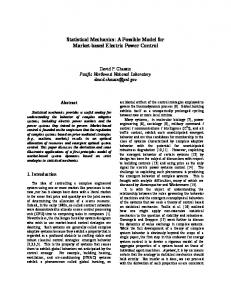
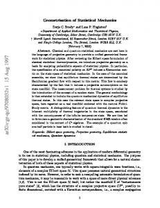
We have seen by property 0a that the pressure at finite volume pΛ (β, λ) is analytic as a function of its parameters β and λ in the whole physical domain λ > 0, β > 0. We can now ask if the infinite volume pressure p(β, λ) is also analytic in its parameters. If this were the case then we would be really in trouble and we should conclude that statistical mechanics is not sufficient to describe the macroscopic behaviour of a system with a large number of particles. As a matter of fact experiments tells us that the physical pressure can indeed be non analytic. For example the graphic of the pressure versus the density at constant temperature (if the temperature is not too high, i.e. not above the critical point) for a real gas is drawn below. When ρ reaches the values ρ0 the gas starts to condensate to its liquid phase and during the whole interval [ρ0 , ρ1 ] the gas performs a phase transitions. i.e. from its gas phase to its liquid phase, at the same pressure p0 . Above ρ1 the system is totally in its liquid phase. The change occurs abruptly and is usually characterized by singular behaviour in thermodynamic functions. Hence, in spite of the fact that pressure is continuous even in the limit, its derivatives may be not continuous in the infinite volume limit. Note that this fact substantially justifies the necessity to take the thermodynamic limit. Until we stay at finite volume, all thermodynamic functions are analytic, hence in order to describe a phenomenon like phase transition we are forced to consider the infinite volume limit. Of course the infinite volume is always taken in such way that ρ = N/V is fixed. We can thus give the following mathematical definition for phase transition Definition 2.3 Any non analytic point of the grand canonical pressure defined in (2.15) occurring for real positive β or λ is called a phase transition point. People believe in general that the pressure p(β, λ) is a piecewise analytic function of its parameters in the physical interval λ > 0 β > 0. Hence it is very important to see which are the values of parameter λ and β for which the pressure is analytic. Guided by the physical intuition low values for λ and β sufficiently low one expects that the pressure is indeed analytic. In fact λ low means that the system is at low density, while β low means that the
2.10. ANALITICITY OF THE PRESSURE
53
Figure 9. Pressure versus density for a physical gas. The gas-liquid phase transition
system is at high temperature (e.g. above the critical point thus so high that the system is always a gas and never condensates). For such values the system is indeed a gas and in general very near to a perfect gas. I.e. for temperature sufficiently high and/or density sufficiently the system is in the gas phase and no phase transition occurs. Hence it should exist a theorem stating that the pressure p(β, λ) is analytic for β and/or λ sufficiently small. We would see later such a theorem. We may ask the following question. We know that p(β, ρ) is continuous while ∂p ∂p e.g. ∂ρ may be not. But if ∂ρ is not continuous in some point it means that at that point ρ0 the function can take two values. So what is the thermodynamic ∂p limit when ρ = ρ0 ? Or, in other words which of the possible values of ∂ρ the system chooses at the thermodynamic limit?. The answer to this question stays in the concept of boundary conditions. Up to now boundary conditions where ”open”, i.e. we were studying a system of particles enclosed in a box Λ supposing that outside Λ there were nothing. In this situation one says that the boundary conditions are open. But of course we could also have done things in a different way, or in more proper words we could have put a different boundary condition . For instance we can put outside Λ n particles at fixed point y1 , . . . , yn . In this case the grand canonical partition function looks as ∫ ∫ ∞ ∑ λN Ξy (β, Λ, λ) = 1 + dx1 . . . dxN e−βU (x1 ,...,xN ) e−βW (x1 ,...,xN ,y1 ,...,yn ) N! Λ Λ N =1 (2.27) where N ∑ n ∑ W (x1 , . . . , xN , y1 , . . . , yn ) = V (xi − yj ) i=1 j=1
54
CHAPTER 2. THE GRAND CANONICAL ENSEMBLE
Figure 10.
Hence the function Ξ(β, Λ, λ) may depend also from boundary conditions. This means that also pΛ the pressure at finite volume depends on boundary conditions. Does the infinite volume pressure depend on boundary conditions? The answer to this question must be no (always guided by physical intuition), at least for not too strange systems and/or not too strange boundary conditions. It is possible to show this quite easily for a finite range ( with range r¯) hard core (with hard core a) potential. I,e particles must stay at distances a or higher and they do not interact if the distance is greater than r¯. In this case particles outside Λ than give contribution to the partition function (2.27) are just in a frame of radius r¯ outside Λ. Supposing that Λ is a cube of size, the volume of this frame is of the order L2 r¯ L. Any particle inside Λ can interact just with particles inside a sphere of radius r¯ centers at the particles position, and due to the hard core condition in this sphere one can arrange at most of the order of (¯ r/a)3 . This means that a particle inside can interact at 3 most with (¯ r/a) particles outside Λ. On the other hand particles inside Λ that can interact with particles outside Λ are also contained in a (internal) frame of size ρ¯, and the maximum number of particles inside Λ(hence contributing to W in (2.27)) is of the order L2 r¯ a3 With this observations it is not difficult to see that |W (x1 , . . . , xN , y1 , . . . , yn )| ≤ Const.
L2 r¯ ( r¯ )3 a3 a
Thus 1 1 L2 r¯ ( r¯ )3 1 ln Ξ (λ, β, λ) = ln Ξ (λ, β, λ) ± Const. υ open L3 L3 L3 a3 a and the factor
L2 r¯ ( r¯ )3 1 Const. L3 a3 a
2.10. ANALITICITY OF THE PRESSURE
55
goes to zero as L → ∞. I.e. the pressure does not depend on boundary conditions. But now in general the derivative of the pressure may depend on boundary condition. This happens precisely when the derivative are not continuous. In such points different boundary condition may force different values of derivatives. Changing boundary condition one can thus change the value on a derivative in a discontinuity point. This can be interpreted as an alternative definition of phase transition. Definition 2.4 A phase transition point is a point in which the value of some derivative of the infinite volume pressure depends on boundary condition even at the thermodynamic limit. Thus when the system is sensible to change of boundary condition even in the infinite volume limit we say that there is a phase transition. By this rough discussion we see that lack of analiticity of the pressure or sensitivity of the system to change in boundary conditions are two ways to characterize a phase transition.
56
CHAPTER 2. THE GRAND CANONICAL ENSEMBLE
Chapter 3
High temperature low density expansion 3.1
The Mayer series
We now come back to the affirmation that a system of particles, interacting via a reasonable potential energy (e.g. defined via a stable and tempered pair potential) should look as a gas at sufficiently low density and/or sufficiently high temperature, hence the pressure of such system should be analytic in the thermodynamic parameters in this region. Since we are consider just the Grand Canonical ensemble, the region of high temperature and low density will be in the case the region of λ small and β small. Let us thus consider again the grand Canonical partition function ∫ ∫ ∞ ∑ λN Ξ(β, Λ, λ) = 1 + dx1 . . . dxN e−βU (x1 ,...,xN ) (3.1) N! Λ Λ N = 1
with
∑
U (x1 , . . . , xN ) =
V (xi − xj )
(3.2)
1≤i