My accompanist at the University is Marijn Huijbregts, who is doing his PhD research on automatic speech recognition. He also created the SHOUT toolkit which ...
Clustered acoustic modelling in speech recognition
!
Door: Begeleiders:
Datum:
Pieter van Veelen Marijn Huijbregts Roeland Ordelman Arjan van Hessen 27 oktober 2007
Preface This report was written as conclusion of my study Computer Science at the University of Twente. It was done internally at the Human Media Interaction chair of the EWI faculty. This research is part of the automatic speech recognition project. My accompanist at the University is Marijn Huijbregts, who is doing his PhD research on automatic speech recognition. He also created the SHOUT toolkit which I used to perform the speech recognition for this project. I would like to thank Marijn for the time, assistance and knowledge during my research. I would also like to thank Roeland Ordelman and Arjan van Hessen for their help and shaping of my assignment. Pieter van Veelen
Summary Speech recognition uses statistical models to compute the most likely spoken sentence from a given audio input. An acoustic model is used for examining the input and a grammar or language model uses knowledge about the language for which sequence of words is most likely to be said. The focus in this research is on the possible ways to improve the acoustic model. An acoustic model is created by taking audio recordings of speech and their text transcriptions, and using software to create statistical knowledge about the sounds that make up each word. This process is called the training of the acoustic model. When an acoustic model is used on another domain (i.e. other speakers or other acoustic environment) than on the domain that it was trained for, it can be enhanced through acoustic model adaptation with the use of adaptation data from the new domain. Different adaptation techniques exist and the effect of the adaptation is influenced by the amount of adaptation data. When the adaptation data consists of a single speaker, a general speakerindependent acoustic model can be transformed into a speaker-dependent acoustic model. When enough adaptation data is available in the new domain for every single speaker, it is possible to create a speaker-dependent acoustic model for every speaker. Because of its focus on one speaker, speaker-dependent systems achieve better results than speaker-independent systems. Thus the logical thing to do seems to always use speaker-dependent models. Unfortunately, there isn’t always enough adaptation data available to create a speaker-dependent model for every speaker in a new task. Another problem could be that creating an acoustic model for every speaker takes up too much processing time. The technique of clustered acoustic modelling can be used as a solution for these problems. With clustered acoustic modelling, all adaptation data is automatically divided into a few clusters, based on properties of the audio data. Hereafter an acoustic model is adapted for every cluster. In this research, the possibilities and performance of clustered acoustic modelling were investigated. The domain for this project was radio broadcasts of Dutch news, a part of the Corpus Gesproken Nederlands (CGN) database. The adaptation method that was used is the SMAPLR adaptation. The first part of this research consisted of tuning some parameters of SMAPLR. First the C factor, a parameter that is used in SMAPLR to control the effect of both the adaptation data and the prior distribution on the adaptation. Next, the minimal amount of data to perform robust model adaptation was determined. The second part is the testing of the clustered acoustic modelling algorithm. Three different scenarios where discussed: 1. Unsupervised clustering and model adaptation 2. Speech recognition with a pre-clustered model 3. Unsupervised adaptation on a pre-clustered model A pre-clustered model is created off-line with the use of supervised adaptation data. The results of the experiments were however rather disappointing. Speech recognition with the clustered models performed worse than recognition with a basic acoustic model. Since the technique of clustering should improve speech recognition in theory (which is confirmed by previous research), we assign this bad results to either unfit data or a software problem. Since the idea of clustered modelling is promising, it is highly recommended to continue research in this area. Especially the results of unsupervised adaptation on a pre-clustered model ought to be interesting. For this reason, this paper is concluded with recommendations for future work on clustered acoustic modelling.
Table of contents Clustered acoustic modelling .............................................................................................................. 1 Preface.................................................................................................................................................... 2 Summary ................................................................................................................................................ 3 Table of contents ................................................................................................................................... 4 1. Introduction........................................................................................................................................ 6 2. Objective............................................................................................................................................. 7 3. Theory................................................................................................................................................. 8 3.1 Speech recognition ........................................................................................................................ 8 3.1.1 Language model...................................................................................................................... 8 3.1.2 Acoustic model ........................................................................................................................ 9 3.1.3 Combining the models .......................................................................................................... 10 3.1.4 Speaker-dependent versus speaker-independent acoustic models ..................................... 11 3.2 Acoustic model adaptation........................................................................................................... 11 3.2.1 Indirect model adaptation ...................................................................................................... 11 3.2.2 Direct model adaptation ........................................................................................................ 12 3.2.3 Combining indirect and direct model adaptation................................................................... 13 3.2.4 Tree-based model adaptation ............................................................................................... 13 3.2.5 SMAPLR adaptation.............................................................................................................. 14 3.2.6 C factor .................................................................................................................................. 15 3.2.7 Number of tree layers............................................................................................................ 16 3.2.8 Supervised versus unsupervised adaptation ........................................................................ 16 3.3 Clustered acoustic modelling ....................................................................................................... 17 3.3.1 Speaker diarization................................................................................................................ 17 3.3.2 Optimal quantity of adaptation data ...................................................................................... 17 3.3.3 Clustering algorithm .............................................................................................................. 18 3.4 Use cases of clustered acoustic models...................................................................................... 18 3.4.1 Basic clustering and adaptation ............................................................................................ 18 3.4.2 Using a pre-clustered acoustic model ................................................................................... 19 4. Experiments ..................................................................................................................................... 22 4.1 Software ....................................................................................................................................... 22 4.2 Domain......................................................................................................................................... 22 4.3 Metrics.......................................................................................................................................... 22 4.4 Tuning the SMAPLR adaptation: optimal amount of adaptation data ......................................... 23 4.4.1 Hypothesis............................................................................................................................. 23 4.4.2 Procedure .............................................................................................................................. 23 4.4.3 Results .................................................................................................................................. 24 4.5 Tuning the SMAPLR adaptation: C factor.................................................................................... 24 4.5.1 Hypothesis............................................................................................................................. 25 4.5.2 Procedure .............................................................................................................................. 25 4.5.3 Results .................................................................................................................................. 25 4.6 Clustered acoustic modelling: baseline experiments................................................................... 25 4.6.1 Hypothesis............................................................................................................................. 26 4.6.2 Procedure .............................................................................................................................. 26 4.6.3 Results .................................................................................................................................. 26 4.7 Unsupervised clustering and adaptation...................................................................................... 26 4.7.1 Hypothesis............................................................................................................................. 26 4.7.2 Procedure .............................................................................................................................. 26 4.7.3 Results .................................................................................................................................. 27 4.8 Speech recognition with a pre-clustered model........................................................................... 27 4.8.1 Hypothesis............................................................................................................................. 27 4.8.2 Procedure .............................................................................................................................. 27 4.8.3 Results .................................................................................................................................. 27 5. Future work ...................................................................................................................................... 29 5.1 Unsupervised adaptation on a pre-clustered model .................................................................... 29 5.1.1 Hypothesis............................................................................................................................. 29 5.1.2 Procedure .............................................................................................................................. 29
5.1.3 Considerations ...................................................................................................................... 29 6. Conclusion ....................................................................................................................................... 30 7. Recommendations .......................................................................................................................... 31 7.1 Unsupervised adaptation on a pre-clustered model .................................................................... 31 7.1.1 Unsupervised clustered adaptation....................................................................................... 31 7.1.2 The adaptation of a pre-clustered model .............................................................................. 31 7.1.3 Re-clustering a pre-clustered model ..................................................................................... 31 7.2 Determining the effect of a maximum tree depth......................................................................... 31 7.3 Pre-clustered model: manually creating clusters ......................................................................... 31 8. References ....................................................................................................................................... 32
1. Introduction Speech recognition is more and more used nowadays, in computer science as well as in every day life. This means that good performance of speech recognition systems becomes more and more valuable. This leads to a lot of research in the speech recognition area. A commonly used speech recognition system processes an acoustic input (spoken words) and gives the most likely spoken sentence as output. The speech recognition uses several components to compute this most likely sentence. Research for improvement is done on all of these components. Two statistical models are used to compute the most likely words that were said from a given audio input. A language model is used to compute the probability of a certain word, based on previous words. For example, the word lamp has a higher probability than the word camp, if the previous words were turn on the. An acoustic model uses knowledge about the acoustic form of words to examine spoken data. The acoustic model has learned this knowledge by looking at training data. When such an acoustic model is used for another task than the domain it was built for, the performance of the speech recognition will decrease. This problem can be avoided by adapting the acoustic model on available adaptation data belonging to the domain of the new task. There are certain options for acoustic model adaptation. The best way is to divide the available adaptation data into different speakers and adapt an acoustic model for every single speaker. These models are called speaker-dependent acoustic models. The disadvantage of this method is that it requires a reasonable amount of adaptation data for every speaker to make the adaptation profitable, which might not be available. This method also takes up a lot of processor time, since the adaptation process is quite lengthy. Another method could be adapting a single acoustic model on all available adaptation data, which makes the model task dependent (or speaker-independent). The disadvantage with this method is that, if the data contains a lot of different speakers, it doesn’t perform quite as well as a collection of speaker-dependent acoustic models. In this research, a possible alternative for speaker-dependent and task dependent acoustic modelling is examined. In stead of adapting a single acoustic model or adapting an acoustic model for every speaker, we will divide the incoming data in different clusters. This division is done on basis of the properties of the audio data. Afterwards, for every cluster a basic acoustic model is adapted on the data belonging to that cluster. This process is called clustered acoustic modelling. The advantages of this method are that every new acoustic model is adapted on a certain minimum amount of adaptation data to make every adaptation profitable, while the total number of clusters (and thus of acoustic models) is controllable.
2. Objective The objective of this research is exploring the possibilities of clustered acoustic modelling. The first step in when applying this technique is, like in speaker-dependent modelling, dividing the adaptation data into different speakers. This is done by a process called speaker diarization, which will be explained in chapter 3. Next, all clusters that contain not enough data to make acoustic adaptation useful are merged with other clusters. This other cluster is selected on the basis of similarity of adaptation data. In order to control the processor time that is needed for adaptation, it is also possible to set the maximum amount of clusters. Since processor time is not an issue for this research however, we will not make use of this option. When all clusters are of appropriate size, the system will then adapt a baseline acoustic model for every cluster on the adaptation data belonging to that cluster. It is obvious that the amount of adaptation data per cluster is an important issue in this research. Because of this, the first step of this project will be defining what the optimal amount of data is to make acoustic model adaptation useful. Next, the result of this will be used to perform clustered acoustic model adaptation. The expectations of this research is, that the speech recognition based on a clustered acoustic model will perform better than the recognition based on a acoustic model that is adapted on all available adaptation data. It is however unlikely that it will perform as well as speech recognition with the use of speaker-dependent acoustic models. The research on clustered acoustic modelling should eventually strive to approach the performance of speaker-dependent modelling.
3. Theory Automatic speech recognition is the process of converting a digitally captured acoustic signal to text. In this chapter, the general working of automatic speech recognition will be explained. Next, the process of acoustic adaptation will be looked at and finally clustered acoustic modelling is discussed.
3.1 Speech recognition When applying automatic speech recognition, the objective is to map an acoustic signal to a set of words. We define the acoustic input as a sequence of observations: O = o1, o2, o3,..., on We will assume that the output of the speech recognition is a sentence, consisting of a sequence of words: W = w1, w2, w3,..., wn Speech recognition uses statistics to compute the best possible outcome. The objective is to find the most likely sentence out of all possible sentences in our language, given a certain acoustic observation. This best outcome can be expressed as follows:
B arg max P(W | O) W
P(W|O) is the probability that a certain sequence of words W was pronounced, given the observation O. This formula arg max P (W | O ) gives us the sentence B, where the probability P(W|O) is maximal. Because the number of all possible sentences in our language is infinite, this formula cannot be computed directly. We use Bayes’ rule to break down the formula:
P( x | y)
P( y | x) P( x) P( y )
Substituting this in our formula:
B arg max W
P(O | W ) P(W ) P(O)
P(O) is the probability of this particular observation. This is however the same value for every possible sentence W. Since we only want to know the sentence with maximal probability, we can simply ignore P(O):
B arg max P(O | W ) P(W ) W
To compute the components of this formula, two statistical models are used. The computation of P(W) is done with a language model and P(O|W) with a acoustic model. These models are explained in the next paragraphs.
3.1.1 Language model Because P(W) is computed using statistical knowledge about the language and is not affected by observations, it is called the prior probability. Since P(W) is the probability that a particular sentence W was spoken, a model is used that is based on the statistical knowledge about the language. We call such a model a language model (LM), or grammar. The most common way to construct a LM is an Ngram LM. This N-gram LM uses the last N-1 words to compute the likelihood of the current word. For
example, a bigram LM uses the previous word to predict the next word and a trigram LM uses the previous 2 words. The construction of such a grammar is done by counting words and its predecessors in large corpora.
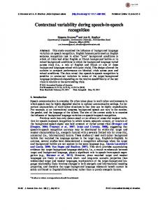
3.1.2 Acoustic model Now we know how to calculate the prior probability P(W), the next step is computing the value for the probability P(O|W). This is the probability that a certain acoustic input O was heard, given that the sentence W was pronounced. The value of this probability can be estimated by making use of an acoustic model (AM). The building blocks of an acoustic model are phones, like n, iy or d (who together form the word need). A typical AM contains about 50 different phones, each of them represented by an acoustic model. These models are usually trained on large amounts of data in order to compute the probability that the relevant phone occurred. Next, the system uses a pronunciation dictionary, or lexicon, to combine phones into words. This is a matter of tying the models for the phones together into a word model, as illustrated in figure 3.2.
n
iy
d
need
Figure 3.2: From phone models to a word model
The same can be done to combine words into sentences. This is illustrated in figure 3.3.
I
need
the
I need the
Figure 3.3: From word models to a sentence
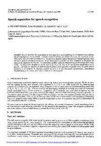
This would mean however that we still need to make a model of an infinite amount of sentences. To overcome this problem, the system creates a pronunciation dictionary which contains most words in our language. An example of such a pronunciation dictionary is illustrated in figure 3.4. When a certain observation is examined, the system walks through the dictionary to map the observation onto a word. To make this process more efficient, words that start with the same phone(s) are put together. This is depicted in figure 3.5. Because of its tree-structure, this pronunciation dictionary is also called a lexical tree.
i
“I”
i
n
iy
d
“need”
n
o
t
“not”
n
o
d
“nod”
th
e
“the”
th
a
n
“than”
th
a
t
“that”
n
th
Figure 3.4: Linear pronunciation dictionary
“I” iy
d
“need”
o
t
“not”
d
“nod”
e
“the”
a
n
“than”
t
“that”
Figure 3.5: Pronunciation dictionary
3.1.3 Combining the models To combine words into sentences, the system simply loops several times through the lexical tree. The lexical tree is used to compute the probability P(O|W). After each loop, the language model is used to compute the probability P(W) for the word that was found. These two probabilities are multiplied with each other to compute the value for P (O | W ) P (W ) . The entire process is illustrated in figure 3.6.
Acoustic model
Speech
Dictionary
Lexical tree
Language model
LM
Text
Figure 3.6: From speech to text
The presence of P(W) in the formula makes it possible to find the correct solution even if the pronunciation or the quality of the data is bad. For example, it could be possible that the first
recognition isn’t correct, but the second one is. This mistake can be corrected with the use of a good language model.
3.1.4 Speaker-dependent versus speaker-independent acoustic models When an acoustic model is trained on data belonging to a single speaker, the model is called a speaker-dependent (SD) model. SD models have the benefit that they perform speech recognition very good for the speaker that they were trained for [5]. Next to their dependency on a single speaker, SD models also have the benefit that they are attuned to the acoustic environment of the training data, like noise or resonance. The counterpart of an SD model is a model that is trained on data that contains multiple speakers. Such a model is called a speaker-independent (SI) model. SI models have the benefit that they are better able then SD models to recognize speech from people whose speech the system has never seen before. SD models usually outperform SI models on a task containing a single speaker (the speaker that the SD model was trained for). SD modelling has its drawbacks however. When it is applied on a task containing multiple speakers, a lot of data has to be available per speaker to train an SD model for every speaker. Such an amount of data might not be available. A solution to this problem is acoustic model adaptation, which will be explained in the next chapter.
3.2 Acoustic model adaptation The model parameters of an acoustic model are set during training. This training process is done on a large amount of data. The performance of speech recognition decreases when recognizing different speakers than the ones in the training data, as was mentioned in the previous chapter. This problem also arises when the acoustic environment changes (e.g. different noise or resonance). To overcome this problem, the acoustic model parameters can be altered by adapting them to new data. This process is called acoustic model adaptation. In the rest of this chapter, we will consider the acoustic model as a set of phones and acoustic adaptation as a transformation of these phones. Adaptation of acoustic models can generally be divided into direct and indirect approaches. These techniques will be explained in the next paragraphs.
3.2.1 Indirect model adaptation Indirect model adaptation techniques generally use a function to transform the parameters of the acoustic model. Since this means that all the model parameters are simultaneously adapted based on the same transformation, this technique is also called global adaptation. Indirect model adaptation is illustrated in figure 3.7 A common implementation of an indirect model adaptation technique is maximum likelihood linear regression (MLLR). In MLLR, the parameters of the transformation function are estimated via maximum likelihood [6]. Indirect MLLR adapts all phones for every transformation, no matter how small the amount of available adaptation data. This makes the method quite efficient when not a lot of adaptation material is available. The downside on MLLR is its poor asymptotic behaviour [6]. This means that the improvement of adaptation quickly becomes almost zero when the amount of adaptation data increases.
Model transformation (e.g. MLLR)
iy
n
d
o iy
n Initial phones
d Adapted phones
o
Figure 3.7: Indirect adaptation (e.g. MLLR adaptation)
3.2.2 Direct model adaptation Different from the indirect adaptation is the direct way for acoustic model adaptation. With direct model adaptation, the new model parameters are often estimated through Bayesian learning . This learning technique is often implemented via maximum a posteriori (MAP) estimation [6]. Direct MAP adaptation uses the information provided by the adaptation data as well as prior knowledge about the model parameters to directly reestimate the relevant model parameters. This means, that only the models that are present in the data are adapted. This process is illustrated in figure 3.8.
iy
n
Initial model
n
iy
d Model transformation (e.g. MAP)
o d
Adapted model
Unadapted model
Figure 3.8 Direct adaptation (e.g. MAP adaptation) Direct model adaptation has the property that every phone is adapted on data that is specific for that phone, meaning that such a phone gets well adapted to the new data. The result of this is that the performance of the adaptation will increase when the amount of adaptation data increases. In that case, the prior knowledge about the model parameters becomes negligible in comparison with the observed data and the model will approach the performance of a speaker-dependent model. The
downside of direct adaptation is that phones that are absent in the adaptation data don’t get adapted at all.
3.2.3 Combining indirect and direct model adaptation As we have seen, both indirect and direct model adaptation techniques have their benefits and drawbacks. Researchers have been focussing on combining these two methods [6], [10]. Another field of research tries to provide additional information to influence the adaptation. An example of this can already be found in MAP adaptation, which uses prior knowledge about the transformation parameters to constraint the estimation based on the adaptation data. Another way of providing additional information, is structuring the model transformations in a tree. This technique is applied in the structured version of the MAP algorithm (structural maximum a posteriori linear regression, or SMAPLR), which is explained in the next chapter.
3.2.4 Tree-based model adaptation We have seen that in standard MAP adaptation every phone is adapted on phone specific data. When there is no adaptation data available for a certain phone (which can be the case if the amount of adaptation data is limited), the phone doesn’t get adapted. Structural maximum a posteriori linear regression (SMAPLR) is organized in such a way to overcome this problem [7]. In global adaptation techniques, like MLLR adaptation, all phones are adapted using the same transformation function. This leads to a very general adaptation, with little gain if the amount of adaptation data is large [6]. This process can be improved by dividing the phones into different clusters[7]. A cluster should then contain phones that are acoustically close to each other, since it seems reasonable that these phones share the same transformation. This principle can be implemented in a tree. The root node contains all phones in the language. The phones are further split down the tree, until each leave contains a single phone. An example of this is illustrated in figure 3.9, where every circle is a node in the tree.
iy
iy
n
iy
d
o
o
n
iy
n
d
d
Figure 3.9 Tree-based division of phones During adaptation, all data is spread over the nodes of this tree. To guarantee useful adaptation, a predefined threshold is used to define what is called a cut. The cut is a set of nodes, such that every subtree contains a (predefined) minimum amount of adaptation data. The transformation parameter for every phone in the original tree is than based on the adaptation data of the closest node in the cut. An example can be seen in figure 3.10. This method is called tree-based MLLR adaptation.
iy
n
iy
d
o
Cut
o
iy
n
iy
d
n
d
Figure 3.10 Tree-based MLLR adaptation, containing a cut of nodes For every node: B arg max P (O | W ) W
The performance of this technique is very dependent on the selection of the threshold. If it is too small, phones might get adapted on a too small amount of data, which could lead to overfitting to the data. On the other hand, a large value for the threshold could lead to a limited amount of different transformations, which constrains the effect of the adaptation. In MAP adaptation, a prior density is added to the transformation to constrain the adaptation. This principle can also be applied to treebased adaptation. In each node in the cut, a prior density is available to constrain the adaptation in that node. This takes care for a more reliable estimation of the transformation parameters. To do this, the maximum likelihood function from the structured MLLR method is replaced with a maximum a posteriori estimation. This is called the MAPLR algorithm, [11]. Applying MAPLR instead of MLLR, we get tree-based MAPLR, which is illustrated in figure 3.11. P(W)
P(W)
iy
iy
n
iy
d
o
Cut
o
n
iy
n
d
d
Figure 3.11 Tree-based MAPLR with prior density for every node in the cut For every node: B arg max P (O | W ) P (W ) W
The advantage of tree-based MAPLR over tree-based MLLR is that in case of a limited amount of adaptation data, the estimation of the transformation parameters are mainly influenced by the prior distribution in each node. This prevents overfitting to the adaptation data.
3.2.5 SMAPLR adaptation An important issue with tree-based MAPLR is the estimation of the prior distribution. How should this value be computed? A solution in [11] suggests that the prior distributions can directly be derived from
the speaker-independent models. Although this method performs better than MLLR adaptation and reduces the dependency on the amount of adaptation data, it is a rather rude method, which doesn’t benefit from the tree-structure [7]. A more dynamic way is proposed in [7], where the tree-structure is also used to share prior information among different nodes. This method makes use of Bayesian statistics. Let’s say that the tree contains a node N with prior distribution P(Wn) and adaptation data On. The posterior distribution of the phones in N can be written down as P(Wn|On). The prior distribution of a child node C of node N is defined by the posterior distribution of node N. This means that P(Cn) = P(Wn|On). This process is illustrated in figure 3.12. P(W)
P(W)
iy
iy
n
iy
d
o
Cut
o
n
iy
n
d
d
Figure 3.12 Tree-based SMAPLR For every node in the cut: Bi arg max P (Oi | Wi ) P (Wi ) W
with
P (Wi ) P (O j | W j ) , where j is the parent node of i
The initial prior distribution (i.e. the prior distribution for the root node, P(W1)) is defined as the identity matrix. Such a dependency between nodes provides a reliable way to compute transformation parameters. If the amount of data is limited, posterior distributions are still reliable enough near the top of the tree, where the most adaptation data is. This reliable posterior distribution is passed as prior distribution down the tree. On lower nodes, this prior distribution is scarcely modified because of the small amount of adaptation data, which make the posterior distribution on lower nodes still reliable. This prevents overfitting to small amounts of adaptation data. However, if the amount of adaptation is large, the prior distributions will get more adapted down the tree to the local adaptation data, which provides for more refined local transformations.
3.2.6 C factor In order to control the role that the prior distribution and the adaptation play in computing the posterior distribution for a certain node in the tree, the prior density is scaled by a scalar coefficient C. This is done in such a way that if the factor C increases the influence of the prior distribution increases. But if C decreases, the influence of the prior distribution decreases and the transformation parameters depend mostly on the adaptation data. This leads to the expectation that SMAPLR adaptation on a large amount of data performs best with a low C factor and vice versa. This is confirmed in [7]. Because of rather significant differences in performance with varying C factor (up to 6% in [7]), tuning the value when setting up a speech recognition system with SMAPLR adaptation is important. The higher nodes in the tree contain more adaptation data than lower nodes. Because of this, the adaptation in higher nodes can depend more on adaptation data and less on the prior distribution. The value of the C factor should thus be low on higher nodes (C equals the aforementioned tuned value at the root node) and high on lower nodes (C approaches 1 at the leaves).
3.2.7 Number of tree layers To compute the value of the C factor for the lower nodes, a certain formula is used. For the software used in this research, this formula is defined as follows:
C _ factor (1.0 initial _ c) * (layer 1) (max_ tree _ depth 1) 0.01 With initial_c is the in chapter 3.2.6 mentioned tuned value, layer is the current layer in the tree and max_tree_depth is the maximum number of layers in the tree. This last value has therefore to be set. Previous researchers in the field of structural model adaptation don’t mention the number of layers in the tree. It is either not mentioned at all (e.g. in [7]), or the number of layers in the tree is mentioned, but not why that particular tree depth was chosen (e.g. in [1], where a tree of 5 layers is used and [12] with a maximum of 8 layers). This means that the effect of the number of layers is unknown, so it could prove to be useful to test this value, in order to improve the SMAPLR adaptation.
3.2.8 Supervised versus unsupervised adaptation A workflow diagram of a general acoustic model adaptation method is illustrated in figure 3.13.
Reference text
Alignment text & audio
Audio
Aligned data
Adaptation
Adapted AM
Basic AM
Figure 3.13 Supervised AM adaptation diagram For such an adaptation, a reference of the text in the adaptation data is needed. This reference contains the words that were actually said. Because this reference is manually created, this type of adaptation is called supervised adaptation. The first process, Align text on audio, maps the reference text on the audio in order to determine what was exactly said. In practice, such a reference file is not available most of the time, which makes supervised adaptation not possible. The solution here is to perform speech recognition with the use of the old acoustic model and use the outcome of this as a reference file. This process is called unsupervised adaptation. This is illustrated in figure 3.14.
Reference text
Aligned data
Alignment text & audio
Audio
Adaptation
Adapted AM
Basic AM
Speech recognition Figure 3.14 Unsupervised AM adaptation diagram In this case, the reference file lacks the quality of the manually made reference, so the performance of unsupervised adaptation is less that of supervised adaptation [6]. Keeping in mind that manual references are often not available, unsupervised adaptation is a frequently used process.
3.3 Clustered acoustic modelling As we saw in the previous chapter, speaker-dependent models outperform speaker-independent models for single-speaker tasks. Speaker-dependent models require however a large amount of training data. A compromise between a speaker-independent model and for every speaker a speakerdependent model is making use of a clustered acoustic model. This means that the there are multiple acoustic models, each focusing on a group of speakers (this is called a cluster). To do this, a speaker clustering algorithm is used to divide the speakers into clusters of speakers. Next, each cluster gets its own acoustic model. There are two ways to do this. First, every acoustic model can be trained from scratch. This requires however a lot of training data per cluster, which might not be available [5]. Because of that, the second possibility is more practical: using a general speaker-independent model and adapting it for every cluster on the available adaptation data [7]. First, there will be a short explanation about how the speakers are divided into clusters. After that follows a more detailed description of the clustering algorithm.
3.3.1 Speaker diarization Speaker diarization is the technique of automatically dividing some acoustic data into different speakers. This technique exists of two steps. The first step is speech activity detection (SAD), to define where speech actually occurs. Next, a speaker diarization algorithm is used to divide the data into different speakers. When applying clustered acoustic modelling, speaker diarization can be used to divide the data into different clusters.
3.3.2 Optimal quantity of adaptation data The performance of acoustic model adaptation is strongly related to the available amount of adaptation data. The question that comes to mind is: how much adaptation data is at least needed, and at which point does more available data means almost no further gain in performance? Previous research in this area is hard to interpret for new projects. It mostly comes as a by-product when evaluating an adaptation technique. Researchers test their speech recognition system and their adaptation technique on a specific domain. However, the performance of their recognition and the gain of their adaptation, and therefore the gain for different amounts of available adaptation data, is very domain-specific.
When testing a new adaptation technique, researchers simply want to compare their technique against other techniques. The measurement of the amount of adaptation data remains mostly unclear and is often expressed in terms like ‘number of utterances’ or ‘minutes per speaker’, without any further explanation (see for example [6] and [7]). Because of the absence of a clear guideline in the literature, it is recommended to test the optimal quantity of adaptation data when starting a new research regarding acoustic model adaptation. When applying clustered acoustic model adaptation, it is important to determine this minimal amount of adaptation to ensure that every cluster gets adapted on a minimum amount of data.
3.3.3 Clustering algorithm As we saw, speaker diarization can be used to divide adaptation data into different speakers. When this is finished, an acoustic model can be trained for every speaker. A problem arises when a speaker occurs with not enough adaptation data (see chapter 3.3.2) to make acoustic model adaptation useful. To overcome this problem, the speakers are combined into clusters, all with a preset minimum amount of data. When the amount of data of a certain speaker is smaller than the minimum amount of data to assure useful adaptation, the data of this speaker will be merged with another speaker, forming a cluster. This other speaker is chosen on basis of similarity of data. This process is continued until every cluster contains a minimum amount of data, which assures that our rule about the minimum amount of adaptation data from chapter 3.3.2 applies for every cluster. This process is illustrated in figure 3.15.
Speech activity detection
Speaker diariztion
Merge small clusters
Merge clusters if too many
Figure 3.15 Clustering algorithm diagram
It is also possible to use a fixed number of clusters in the system. This means that program keeps merging the two most likely clusters, until this fixed number of clusters is reached. This can be useful when enough adaptation data is at hand and you want to create a general model for recognizing unknown new data. This will be further elaborated in the next chapter.
3.4 Use cases of clustered acoustic models Clustered acoustic modelling can be used in many different scenarios. A few of these use cases will be discussed in this chapter.
3.4.1 Basic clustering and adaptation The first question that comes to mind when making use of clustered acoustic models is: what is the actual benefit of this technique? This can be tested easily by performing clustered model adaptation on an existing acoustic model. The performance of this clustered model should then be higher than the performance of the original non-clustered acoustic model. The entire process is illustrated in figure 3.16. 3.16a shows the process of creating a clustered and adapted AM, while 3.16b shows the speech recognition process with this model. The Cluster Info, Clustered AM and (incoming) audio are the same for both figures. The decode action involves a speech recognition task.
Speaker diarization
Cluster info
Decode
Audio
Recognition
Unsupervised clustered adaptation
Basic AM
Clustered AM
Figure 3.16a Clustering and adaptation diagram
Clustered AM
Audio
Decode
Recognition
Cluster info Figure 3.16b Speech recognition with a clustered AM
The first step here is performing speech recognition on the data with the use of a base acoustic model, which produces a recognition. Next, the incoming audio is divided into different clusters through speaker diarization. Then the base acoustic model is being adapted for every cluster, which produces a clustered acoustic model. The aforementioned speech recognition is used as reference for this acoustic model adaptation. Finally, the clustered acoustic model is used to perform another recognition of the data.
3.4.2 Using a pre-clustered acoustic model Another possible use of clustered acoustic models involves an acoustic model that is beforehand clustered. This means that the clustering is performed with the use of training data instead of new task data. This process is depicted in figures 3.17 and 3.18.
Training Data
Speaker diarization
Supervised clustered adaptation
Cluster info
Basic AM
Reference file
Preclustered AM Figure 3.17 Off-line creation of a pre-clustered AM
Here, the basic acoustic model is used to create off-line a clustered acoustic model (figure 3.17). The adaptation of this model is supervised, with the use of a reference file. The first step on-line is determining which cluster has to be used for which segment of the incoming audio through speaker diarization. The clustered model is then used to perform speech recognition on the (figure 3.18). The data that is used for this process is the same as the data that was used for the original training of the acoustic model. This method has some advantages over the one described in the previous chapter. First of all, the clustering is done off-line, which means a faster process online (only one decode action). Another advantage is that the adaptation of the different clusters is now supervised, which makes the adaptation more reliable (see chapter 3.2.8).
Speaker diarization
Audio
Cluster info
Decode
Recognition
Preclustered AM Figure 3.18 Speech recognition with a pre-clustered AM In this case, the speech recognition is done with the use of a general clustered acoustic model. The next logical step in clustered modelling is adapting the pre-clustered model to the incoming data. Here, the first step is again creating a pre-clustered acoustic model, as seen in figure 3.17. Next, this clustered acoustic model is adapted to the incoming audio data (figure 3.19). Finally, this adapted acoustic model is used for the speech recognition task (figure 3.20). The same information from the speaker diarization action in figure 3.19 is used to assign every piece of data into the right cluster for decoding.
Speaker diarization
Audio
Cluster info
Decode
Unsupervised clustered adaptation
Recognition
Preclustered AM
Adapted Clustered AM
Figure 3.19 Adapting a pre-clustered AM When adapting the pre-clustered acoustic model, the first step is to divide the data into the different clusters. After that, every cluster is adapted on its assigned data. The possibility exists that a cluster ends up with a too small amount of adaptation data, as was discussed in chapter 3.3.2. When this is the case, the data of this cluster should be passed to the nearest cluster. This prevents bad adaptation. Audio
Adapted clustered AM
Decode
Recognition
Cluster info Figure 3.20 Speech recognition with an adapted clustered acoustic model
4. Experiments In this chapter, the experiments that were performed for this research will be discussed. The objective of this project, as posed in chapter 2, was used to formulate hypotheses regarding two research problems. The first problem handles the fine-tuning of the SMAPLR adaptation technique, which was used in this research. The second problem, expressed into multiple hypotheses, tests the technique of acoustic modelling based on speaker clustering. The hypotheses are tested by means of experiments. For every experiment, the used datasets, procedure and results are discussed here. The tuning of SMAPLR adaptation is further explained in chapter 4.4 (minimal amount of adaptation data), 4.5 (C factor) and 4.6 (tree depth). Chapters 4.6 to 4.9 contain the use cases that were tested for clustered model adaptation, as explained in chapter 3.4. First, a brief introduction to the software that was used, the domain on which the experiments were performed and the metrics on which the experiment results were evaluated.
4.1 Software The software package that was used to perform the large vocabulary continuous speech recognition for this research is called SHOUT. SHOUT is a speech recognition toolkit developed at the University of Twente. SHOUT uses the SMAPLR acoustic model adaptation technique, which is discussed in chapter 3.3. SHOUT also supports speaker clustering. The clustering is performed at adaptation time, making the adaptation as follows:
The adaptation data is examined and divided into clusters. The data that will be used for these experiments is already divided into small data files, each containing an utterance of a single speaker. Because of this, each data file will be examined and assigned to a certain cluster. The acoustic model that is going to be adapted, is used to align the acoustic data onto its transcription During the actual adaptation, the system recognizes that the adaptation data is divided in clusters and trains an acoustic model for every cluster. These models are stored in one file, a clustered acoustic model
When speech recognition is performed with the use of such a clustered acoustic model, the recognizer automatically divides the task data into the present clusters. The data is then recognized with use of the acoustic model that belongs to its cluster. A detailed description of SHOUT can be found at [9]. Below is a list of the components that were used for the speech recognition and adaptation. All are part of the automatic speech recognition package, developed by the University of Twente. Acoustic model: Language model: Lexicon:
ut-bn2005_02.am.bin 65k.news.lm.bin 65k.news.dct.bin
4.2 Domain The domain on which the experiments are executed is the “Corpus Gesproken Nederlands” (CGN), a large vocabulary corpus of spoken Dutch sentences. The component of CGN that will be used is the recording of Dutch newscasts. The newscasts are divided in a training set, a develop set and an evaluation set. The training of the acoustic model that is used in this project was done with the training set. The develop set is used to perform our experiments and will be divided into an adaptation part and a test part. The evaluation set is not used during this research. For every experiment, the datasets that will be used are described further on in this chapter.
4.3 Metrics To test the performance of a speech recognition system, we simply let it execute a speech recognition task and look at the results. The data which is used for this task cannot be part of the data on which the model was trained or adapted, to assure valid results. We do however have a reference of the task data. The reference text is a transcription of the words that were spoken. This allows us to compare the recognized text with the reference text.
The tool that we use for this comparison is called sclite. This program computes the percentage of words that was incorrectly recognized. This value is called the Word Error Rate, shortly WER. More information about sclite can be found at [8].
4.4 Tuning the SMAPLR adaptation: optimal amount of adaptation data The first experiment handles the testing of the optimal amount of data to make acoustic model adaptation worthwhile. Worthwhile is a somewhat vague term, which we’ll try to explain. The expectation about acoustic model adaptation is that the performance will keep increasing as the amount of adaptation data increases. When testing this adapted acoustic model, its WER will then converge to a certain value. This value differs per task, dependent on matters as acoustic environment, quality of the data and the pronunciation of the speakers. In the context of clustered model adaptation, we want to keep the minimal amount of data per cluster low, which allows us to create as many clusters as possible. The goal of this experiment is thus to find a compromise between good adaptation and little adaptation data. Further experiments on acoustic model adaptation on this domain can be done with supervised adaptation as well as unsupervised adaptation. Because of this, we are going to perform this experiment with both supervised and unsupervised adaptation.
4.4.1 Hypothesis The expected behaviour of acoustic model adaptation on different amounts of data is sketched in figure 4.1. This behaviour is based on every research on acoustic model adaptation [1] [2] [6] [7] [10]. We will define the optimal amount of adaptation data at the point marked with X. This point has the advantage over point Y, because the gain in performance is still worthwhile. The performance at point Z may be slightly better than the performance at point x, but the difference is just minimal and not in the same order of magnitude as the difference in amount of adaptation data. The expectation is that the supervised adaptation performs better than unsupervised adaptation, but both their curves should look like the curve in figure 4.1.
W E R
x
Amount of adaptation data
Figure 4.1 Expected behaviour of acoustic model adaptation for different amounts of data
4.4.2 Procedure As was said in chapter 4.2, we are using the develop set of the newscasts component of the CGN data. This test was divided into two parts: a part for adaptation (75% of the data) and a part for testing (25%). After this, the data is further (manually) divided into different speakers. For every speaker, a WER is determined using a non-adapted acoustical model. This is our baseline WER, to which we will compare the WER we obtain after acoustic model adaptation.
After the baseline experiment, the same acoustic model is adapted on different amounts of data (varying from very little data to all available data). This is done for three different speakers. The experiments are done for supervised and unsupervised adaptation, both times on the same data.
4.4.3 Results The baseline experiments (with the use of an unadapted acoustic model) for the three speakers in this experiment produced the following results: Speaker 02001 02008 02009
Sentences WER 200 29,2% 200 22,6% 184 24,0% Tabel 4.1 Baseline WER
Table 4.2, 4.3 and 4.4 contain the speech recognition results with use of an acoustic model after supervised adaptation with different amounts of data. # sentences WER 3 28,7% 20 26,9% 50 27,0% 75 26,2% 100 25,9% 300 25,1% Tabel 4.2 Speaker 02001
# sentences WER 3 22,3% 20 20,3% 50 20,7% 75 20,3% 100 20,6% 300 20,3% Tabel 4.3 Speaker 02008
# sentences WER 3 28,7% 20 21,8% 50 19,8% 75 20,2% 100 21,7% 184 22,1% Tabel 4.4 Speaker 02009
The results are basically what we expected. The only discrepancy is the increasing performance word error rate for speaker 02009 with a larger amount of adaptation data. This could be attributed to adaptation data of less quality in later sentences. Tables 4.5, 4.6 and 4.7 show the results on the same data, but now after unsupervised adaptation.
# sentences WER 3 29,7% 20 27,1% 50 26,6% 75 26,2% 100 26,1% 300 26,3% Tabel 4.5 Speaker 02001
# sentences WER 3 50,2% 20 23,0% 50 21,9% 75 21,3% 100 21,2% 300 21,8% Tabel 4.6 Speaker 02008
# sentences WER 3 27,7% 20 22,1% 50 21,6% 75 21,5% 100 21,6% 184 21,3% Tabel 4.7 Speaker 02009
The results of unsupervised adaptation follow about the same pattern as unsupervised adaptation, albeit that supervised adaptation performs on average better. Due to the reasons explained in chapter 4.4.1, we have defined the optimal amount of adaptation data at 90 sentences. The difference between 75 or 100 sentences is almost negligible, so an amount of 90 sentences seems like a reasonable amount.
4.5 Tuning the SMAPLR adaptation: C factor The C factor is an important setting for SMAPLR adaptation, because it controls the influence of both the prior distribution and the adaptation data on the adaptation parameters. When there is a lot of adaptation data available, the influence of the prior distribution should be lower, in order to make the must use out of the large amount of adaptation data. On the other hand, with a small amount of adaptation data, the prior distribution should be of more importance to prevent overfitting and adaptation on bad data. In this experiment, we will test the effect of the C factor for different amounts of adaptation data. The results will be used to determine the optimal value for the C factor for further experiments.
4.5.1 Hypothesis Since this experiment is executed in order to tune the value of the C factor, not much can be said about the actual resulting value. However, it will be interesting to see if the results of the adaptation behaves as expected, when changing the value of the C factor The expectations are that a lower C factor will perform better on a small amount of adaptation data (due to an increased influence of the prior distribution) and will perform worse on bigger amounts of adaptation data than adaptation with an increased C factor.
4.5.2 Procedure The C factor tuning is a very straight-forward experiment. The basic acoustic model will be adapted with the SMAPLR algorithm for different amounts of adaptation data. After each adaptation a WER will be determined via speech recognition. This process will be executed for three different values for the C factor. We will start with a C factor of 0,01 (adopted from [7]). Next, we will try a value of 0,1 and 0,001. If a C factor of 0,1 performs better than 0,01, we will continue experiments with higher values for the C factor. If 0,001 performs better than 0,01, we will try experiments with lower values. As was mentioned in chapter 3.2.6, the value of the C factor is automatically adapted through the layers of the tree. The C factor that will be tested here is the value for the root node. The value will get higher for lower nodes, until it reaches 1 in the leaves of the tree. The experiments will be done on data for speaker 02001 from the CGN database. They will be executed for 3, 20, 50, 100 and 300 sentences.
4.5.3 Results The results of speech recognition on models adapted with different C factors are shown in tables 4.8 to 4.10. # sentences WER 3 28,7% 20 26,9% 50 27,0% 100 25,9% 300 25,1% Table 4.8 C = 0,01
# sentences WER 3 28,7% 20 29,2% 50 27,6% 100 25,8% 300 25,3% Table 4.9 C = 0,1
# sentences WER 3 29,7% 20 27,7% 50 27,6% 100 27,3% 300 26,2% Table 4.10 C = 0,001
As can be seen, the adaptation performs best with a C factor of 0,01. Striking in this case is that a lower C factor of 0,001 performs worse on a very small amount of adaptation data (3 sentences). The expectation was that a lower C factor should perform better in this case. This unexpected behaviour could be a result of bad data. Another explanation could be that the quality of the data is in fact very good, which results in a rather good adaptation with a higher C factor. The lower C factor (0,001) gives more weight to the prior information and less to the data, which results in a worse adaptation. The behaviour of the higher C factor (0,1) is rather what was expected. When the amount of adaptation data increases, the results get better than the results of lower C factors. It even performs better on 100 sentences. The fact that is doesn’t perform worse on 3 sentences could again be that these sentences where of good quality, as was explained above. This idea is confirmed in the fact that the speech recognition is better on 3 sentences than on 20 sentences.
4.6 Clustered acoustic modelling: baseline experiments Before performing the experiments regarding clustered model adaptation, we have to execute two baseline experiments in order to give value to later results. First we will perform speech recognition on incoming data, making use of a basic, non-clustered, acoustic model. Next, we will perform unsupervised adaptation on this acoustic model, with the use of the same incoming data. We will also perform speech recognition on the data with this adapted acoustic model.
4.6.1 Hypothesis The expectations for these two baseline experiments are very obvious. The recognition on the adapted acoustic model should outperform the recognition with the non-adapted model. If this hypothesis fails, it could only mean that the amount of data was too small or the data was very bad.
4.6.2 Procedure The procedure for this experiment is almost similar as described in 5.4.2. We are going to use 200 sentences of two different speakers from the CGN corpus: Speaker Adaptation Recognition ID sentences sentences 02001 800 200 02008 800 200 Table 4.11 Division of the data First, speech recognition will be performed on the recognition sentences for both speakers using the basic acoustic model. Second, this acoustic model will be adapted to the adaptation data for every speaker, after which again speech recognition will be performed. Note that the data for these experiments is somewhat different than the data used for experiments in chapter 4.4, whit slightly different baseline results.
4.6.3 Results The results of the baseline experiments are shown in table 4.12 (without adaptation) and 4.13 (with adaptation). Speaker ID WER 02001 29,2% 02008 21,1% Table 4.12 Recognition with a basic AM
Speaker ID WER 02001 27,6% 02008 19,5% Table 4.13 Recognition with an adapted AM
These values will be used to examine the results of further experiments.
4.7 Unsupervised clustering and adaptation The first experiment with the use of a clustered acoustic model is explained in chapter 3.4.1. The incoming data is used for creating a clustered acoustic model. This model is adapted with unsupervised SMAPLR adaptation. Further, speech recognition with this clustered model is performed on the same incoming data.
4.7.1 Hypothesis The result of the speech recognition of this experiment should outperform the baseline experiment without acoustic model adaptation as well as the baseline experiment with acoustic model adaptation. It will be further interesting to compare the performance with the experiments in chapter 4.8 and 4.9.
4.7.2 Procedure The dataset used for the experiment is of course the same as in the baseline experiments: 200 sentences of 2 different speakers. The flowchart of this procedure is depicted in figure 3.14. The following steps have to be taken: 1. Perform speech recognition on the data with a basic acoustic model 2. Divide the data into clusters through speaker diarization 3. Perform clustered adaptation on the basic acoustic model with the recognition from step 1 as reference and the diarization of step 2 for defining the different clusters 4. Perform speech recognition on the data with the clustered acoustic model The SHOUT toolkit performs steps 2 and 3 automatically, resulting in a clustered acoustic model. This model is then used to perform speech recognition on the data (i.e. the same data that was used for the clustering and adaptation). For step 4, the data is again divided over the different clusters. This should be the same division as was determined in step 1, since both times the same algorithm is used.
4.7.3 Results The final WERs after speech recognition can be seen in table 4.14. Speaker ID WER 02001 30,3% 02008 23,5% Table 4.14 Recognition after clustered adaptation The speech recognition was in this case slightly worse than recognition with the basic acoustic model. This problem will be discusses in the next chapter.
4.8 Speech recognition with a pre-clustered model The next step in this research on clustered model adaptation holds the use of a pre-clustered model. For this experiment a pre-clustered acoustic model will be created off-line, which means that clustering and supervised adaptation will be performed on the basic acoustic model. After this, speech recognition will be performed with this model on incoming audio. The entire process is illustrated in figure 3.17 and 3.18.
4.8.1 Hypothesis For this experiment, we are mostly interested in the performance in comparison with the baseline experiment in chapter 4.6 and the clustering experiment in chapter 4.7. Should the use of a preclustered acoustic model perform better than the experiments with an on-line created clustered model, then the use of such a pre-clustered model would is a good step forward in this area of speech recognition. Future research should then explore its possibilities and possible improvements.
4.8.2 Procedure For this experiment, we make use of the same data as was shown in table 4.11. The adaptation data is used for supervised clustering and adaptation. The actions for this procedure are as follows: Off-line: 1. Divide the adaptation set into clusters through speaker diarization 2. Perform clustered supervised adaptation on the basic acoustic model with the diarization of step 1 for defining the different clusters On-line: 3. Divide the adaptation set into clusters through speaker diarization over the different clusters of the in step 2 created clustered acoustic model 4. Perform speech recognition on the data
4.8.3 Results The results of this experiment can be seen in table 4.15. These results are obviously not what we hoped for, since they are a lot worse than our baseline experiments. Speaker ID WER 02001 41,8% 02008 28,2% Table 4.15 Recognition after clustered adaptation The reason of this disappointing outcome is hard to explain. The adaptation technique is the same as was used in 4.4, so we assume that the adaptation isn’t the problem. Another possibility is bad clustering, for example with (most) clusters containing data of both speakers and mixing them up. The division of the adaptation data over the different clusters is shown in table 4.16. Cluster ID SPK06
Speaker (# segments) 02001 (8) 02008 (303) SPK07 02008 (496) SPK11 02001 (791) 02008 (1) Tabel 4.16 Division of adaptation data over the clusters
This seems a healthy clustering, since all clusters contain mostly data of a single speaker. The data of speaker 02008 is apparently divided over 2 clusters, while speaker 02001 has its own cluster. The division of the recognition data is shown in table 4.17. Cluster ID CDM00 CDM01
Speaker (# segments) 02008 (69) 02001 (50) 02008 (131) CDM02 02001 (150) Tabel 4.17 Division of recognition data over the clusters This table shows a flaw for cluster CDM01, which contains a large amount of sentences from both speakers. This could well be the reason of the bad results.
5. Future work Due to the reasons explained in chapter 4.8.3, the experiments for this research came to an end at this point. Another problem arose when the clustering method was executed for a larger amount of data. This led to a crash of the system due to a shortage of memory. When the circumstances are better for performing (off-line) clustered model adaptation, it is recommended to continue research in this area. An interesting experiment (which was the aimed conclusion of this project) will be explained in the next paragraph.
5.1 Unsupervised adaptation on a pre-clustered model For this experiment a pre-clustered acoustic model will be created off-line (see figure 3.17), which means that clustering and supervised adaptation will be performed on the basic acoustic model. After this, the clustered model is again adapted, now unsupervised on the incoming audio (figure 3.19). Finally, speech recognition will be performed on the incoming audio with the adapted pre-clustered model (figure 3.20).
5.1.1 Hypothesis The expectation for this experiment is that it performs better than the experiment discussed in chapter 4.8, since the clustered model is again adapted on the incoming data.
5.1.2 Procedure To compare the results with previous experiments, the same data as in the other experiments has to be used (see table 4.11). First, an off-line clustered acoustic model is created: 1. Divide the adaptation set into clusters through speaker diarization 2. Perform clustered supervised adaptation on the basic acoustic model with the diarization of step 1 for defining the different clusters On-line the following steps are taken: 3. Perform speech recognition on the data with the clustered acoustic model from step 2 4. Divide the data into clusters through speaker diarization 5. Perform clustered adaptation on the clustered acoustic model with the recognition from step 3 as reference and the diarization of step 4 for mapping every sentence into an existing cluster 6. Perform speech recognition on the data with the clustered acoustic model
5.1.3 Considerations The adaptation of a pre-clustered acoustic model has to be done with care. As was mentioned in chapter 3.4.2, the amount of data that is assigned to every cluster should not be too small, in order to prevent bad adaptation. When a cluster ends up with too little data however, a possible solution to this problem is moving this data to the nearest cluster, until all clusters contain enough data. After this, adaptation can be executed for all clusters. Another possibility is not only moving this data to another cluster, but merging the model parameters from the acoustic models belonging to these clusters to create a new acoustic model. This model can then be adapted on the data of the initial clusters. A third solution is to not perform model adaptation for clusters with small amounts of data, but to keep the original acoustic model for that cluster to perform speech recognition. When the incoming data consists of just a single speaker, it is well possible that all data is assigned to a single cluster. This would mean that the clustering was rather pointless. In this case, the acoustic model of the only used cluster could on its turn again be clustered and adapted on the new data. Before applying this, it has to be made sure that unsupervised clustering and adaptation (see chapter 4.7) performs better than unsupervised adaptation without clustering. The process of re-clustering a cluster leads to the idea of performing this process for every cluster, after the incoming data is divided. When a cluster contains enough data, clustering and unsupervised adaptation could be applied. In this case it also has to be certain that unsupervised clustering and adaptation is preferable over unsupervised adaptation without clustering.
6. Conclusion 6.1 Tuning the SMAPLR adaptation parameters The first part of this project, determining and tuning the parameters of the SMAPLR adaptation technique, turned out to be very useful. The influence of the C factor and the optimal amount of data for adaptation can not be neglected. A different C factor can affect the performance of speech recognition up to 2,6%, which is a rather significant gain. Regarding the optimal amount of adaptation data, it is clear that the performance of speech recognition increases while the amount of adaptation data increases. In SMAPLR adaptation, the adaptation data is divided over a tree. The more nodes that are used in the tree, the more precise the adaptation becomes. Therefore, each node should contain as little data as possible, to fill as much nodes as possible. For this reason, a balance has to be found between as many nodes as possible, but still enough data per node.
6.2 Clustered acoustic modelling The general conclusion at the end of this research is that the technique of clustered acoustic modelling is very promising, but the actual performance is still unclear and needs a lot of further testing. Three different uses of clustered modelling were constructed. It still needs to be determined which of these methods gives the best results. In order to make a beginning with the continuation of this research, a step-by-step plan for future work is provided.
7. Recommendations As was discussed in chapter 5, the research in the area of clustered acoustic modelling is not at all completed and further experimenting is strongly recommended. The most important recommendations for continuation are discussed in chapter 5.1.3. The discussion here is summarized in the next paragraph. After that, some other recommendations for further research are discussed.
7.1 Unsupervised adaptation on a pre-clustered model The process of unsupervised adaptation on a pre-clustered model is discussed in chapter 5. Here, a summary of the recommended steps to be taken in future research is given:
7.1.1 Unsupervised clustered adaptation First of all, the performance of unsupervised clustered adaptation has to be tested. It is important for further research if this method outperforms unsupervised adaptation without clustering.
7.1.2 The adaptation of a pre-clustered model The adaptation of a pre-clustered model can be done in different ways. Just adapting every cluster to its assigned incoming data might not always be the best way, since a cluster might contain a too small amount of data. Three possible solutions to this problem are: Move data from too small clusters to the nearest cluster. When every cluster contains enough data, adaptation is performed on the clusters. Merge acoustic models from small clusters. In stead of just throwing a small cluster away, it might also be possible to merge its acoustic models with the acoustic model of the nearest cluster. Don’t adapt small clusters. The third option is to not adapt a cluster which contains too little data. This way, the original clustering is still used, all data is recognized with an acoustic model belonging to the cluster it was assigned to and all model adaptations are robust. These three possibilities should be tested in order to determine the best method.
7.1.3 Re-clustering a pre-clustered model When the incoming data is divided over the different clusters, the task at hand for every cluster is really just a new task with a certain amount of unknown incoming data and an acoustic model. So, when clustered acoustic modelling is the best solution to perform speech recognition on the original task, than clustered acoustic modelling is also the best solution to perform this smaller task for every single cluster. Therefore, the logical next step is re-clustering every cluster on its assigned data. This process is explained in chapter 4.7. This is of course only useful for tasks with a large amount of data. It would also take up a lot of processing time, since a lot of model adaptation has to be performed.
7.2 Determining the effect of a maximum tree depth The value for the maximum tree depth in the SMAPLR adaptation algorithm is used to compute the C factor (see chapter 3.2.7). However, the effect of the value for the maximum tree depth is yet unknown. It might influence the performance (adaptation benefit as well as speed) of the SMAPLR adaptation, so it deserves some research to determine the optimal value.
7.3 Pre-clustered model: manually creating clusters A pre-clustered acoustic model was used for some of the experiments in this research. This model is created automatically, by providing the system with a basic acoustic model and a certain amount of data. The data is divided into clusters and for every cluster the basic acoustic model is adapted. It might however be interesting to perform the division by hand. Possible ways of separating the data is by gender, by tone pitch or by some environmental property.
8. References [1] [2] [3] [4] [5] [6]
[7] [8] [9] [10] [11]
[12]
Sinoda & Lee, Unsupervised adaptation using structural Bayes approach, Proceedings of IEEE workshop on speech recognition and understanding, 1997 Nguyen & Xiang, Light supervision in acoustic model training, ICASSP 2004 Liu & Kubala, Online speaker clustering, ICASSP 2003 Nguyen, Matsoukas, Davenport, Kubala, Schwartz & Makhoul, Progress in transcription of broadcast News using Byblos, ICASSP 2002 Xiang, Nguyen, Matsoukas & Schwartz, Cluster-dependent acoustic modelling, ICASSP 2005, pages 677-680 O. Siohan, C. Chesta, and C.-H. Lee, Joint Maximum a Posteriori Adaptation of Transformation and HMM Parameters, IEEE Trans. on Speech & Audio Proc. Vol. 9, No. 4, pages 417-428, 2001 O. Siohan, T.A. Myrvoll, and C.-H. Lee, Structural maximum a posteriori linear regression for fast HMM adaptation, 2000 http://www.nist.gov/speech/tools/index.htm http://wwwhome.cs.utwente.nl/~huijbreg/shout/ Digilakis & Neumeyer, Speaker adaptation using combined transformation and Bayesian methods, IEEE trans. Speech audio processing vol. 4, July 1996 Chesta, Siohan & Lee, Maximum a posteriori linear regression for hidden Markov model adaptation, proceedings of European conference on speech communication and technology vol. 1 pages 211-214, 1999 Thiele & Bippus, A comparative study of model-based adaptation techniques for a compact speech recognizer, Automatic speech recognition and understanding workshop, 2001