Clustering in Dynamic Causal Networks as a Measure of Systemic Risk on the Euro Zone Monica Billio, Lorenzo Frattarolo, Hayette Gatfaoui, Philippe de Peretti
SYRTO WORKING PAPER SERIES Working paper n. 3 | 2016
This project has received funding from the European Union’s Seventh Framework Programme for research, technological development and demonstration under grant agreement n° 320270. This documents reflects only the author's view. The European Union is not liable for any use that may be made of the information contained therein.
Clustering in Dynamic Causal Networks as a Measure of Systemic Risk on the Euro Zone Monica Billio∗, Lorenzo Fratarollo†, Hayette Gatfaoui,‡ Philippe de Peretti§ February 16, 2016
Abstract In this paper, we analyze the dynamic relationships between ten stock exchanges of the euro zone using Granger causal networks. Using returns for which we allow the variance to follow a Markov-Switching GARCH or a Changing-Point GARCH, we first show that over di§erent periods, the topology of the network is highly unstable. In particular, over very recent years, dynamic relationships vanish. Then, expanding on this idea, we analyze patterns of information transmission. Using rolling windows to analyze the topologies of the network in terms of clustering, we show that the nodes’ state changes continually, and that the system exhibits a high degree of flickering in information transmission. During periods of flickering, the system also exhibits desynchronization in the information transmission process. These periods do precede tipping points or phase transitions on the market, especially before the global financial crisis, and can thus be used as early warnings of phase transitions. To our knowledge, this is the first time that flickering clusters are identified on financial markets, and that flickering is related to phase transitions. Keywords: Causal Network ; Topology ; Custering , Flickering ; Desynchronisation ; Phase transitions. ∗ Department of Economics, University Ca’ Foscari of Venice, Fondamenta San Giobbe 873, 30121, Venice, Italy. † Department of Economics, University Ca’ Foscari of Venice, Fondamenta San Giobbe 873, 30121, Venice, Italy. ‡ IESEG School of Management (LEM-CNRS), Socle de la Grande Arche, 1 Parvis de la Défense, 92044 Paris La Défense and Centre d’Economie de la Sorbonne, University Paris 1 Panthéon-Sorbonne,
[email protected],
[email protected]. § Corresponding author, Centre d’Economie de la Sorbonne, University Paris 1 PanthéonSorbonne, 106-112 Boulevard de l’Hôpital, 75013 Paris. Tel: 00 33 1 44 07 87 63,
[email protected].
1
1
Introduction
Systemic risk has received a great deal of attention over these recent years. Even if there is no unique definition of systemic risk, as emphasized by Bisias et al. (2012), the concept of systemic risk is clearly related to connectedness, contagion, and therefore di§usion of exogenous and/or endogenous shocks within and/or across financial sectors. One natural way to study systemic risk is to start from a network representation, and next to focus on its topology. Studies based on the topology such as Allen and Gale (2000) or Acemoglu et al. (2013) show that highly interconnected networks (i.e. networks with high degrees) are more resilient to small shocks but not to large shocks. Billio et al. (2012) use causal networks and also focus on the degrees (i.e. the total number of connections). They show that increased degrees have predictive contents concerning financial crises. Battiston et al. (2013) focus on the frailty of nodes, and study cascading dynamics such as Motter and Lai (2002) do. In such models, the focus is set on the impact of the failure of one node or several nodes on the whole system. Furthermore, Hackett et al. (2011) and Payne et al. (2009) emphasize the importance of networks’ topology while studying clustered and degree-correlated networks respectively. The scope of this paper is twofold. Focusing on ten stock exchanges within the Euro zone, we first study the di§usion dynamics of shocks. Then, we suggest early warnings of phase transitions or tipping points while focusing on a particular information returned by the topology of networks. It is worth emphasizing that we consider financial networks as being possibly critically self-organized (Bak et al., 1987, Bianconi and Marsili, 2004). In particular, local interrelations between the system’s components build up a coordinated system or network. Such self-organised network/system will turn into a critical behavior (i.e. tipping point and phase transition) without the e§ect of external forces or drivers. In this light, we target to identify phase transition indicators. We adopt a two-step methodology. We first build dynamic causal networks, as suggested by Billio et al. (2012) but we use a di§erent methodology. Our network’s identification relies on a functional connectivity analysis, and more specifically, on a di§erent class of Granger non-causality tests. Indeed, we implement time series tests under the independence test framework (see Hong 1996, Duchesne and Roy, 2001, Koch and Yang, 1986 or El Himdi and Roy (1997), Pham et al. (2001) or Hallin and Saidi (2001) among others). Such tests are performed on normalized innovations of Generalized Auto-Regressive Conditional Heteroskedasticity (GARCH), Markov-Switching GARCH or Changing-Point GARCH models (Bauwens et al. 2014). Independence tests for time series are very versatile tests that allow for analyzing instantaneous correlations, but also non-causality for a given number of lags, or at a given lag. They also allow for building directed and undirected networks, as well as weighted and binary networks. Functional connectivity is very appealing since it allows for capturing the complex interplay between nodes such as feedbacks and spillover e§ects. Also, despite its apparent simplicity, it has been shown by Zhou et al. (2014) in integrate-and-fire neuronal systems (see also Winterhalder et al., 2005) that 2
Granger non-causality is able to capture some non-linear relationships. After networks’ identification, we propose a period-specific analysis of the contagion process within the network while discriminating between crisis and non-crisis periods. Then, we describe dynamically the network’s topology while focusing on the short-term dynamic di§usion process of information/shocks. Using rolling windows, we apply clustering measures (Faggiolo, 2007). In particular, we focus on specific patterns or motifs of information di§usion within the network (i.e. information flow’s spreading). Considering the daily stock index returns of ten stock exchanges within the Euro zone from 1994 to 2014, our findings are fourfold. First, with respect to period-specific analysis, correlations prevail over the data sample while being time-dependent. Such correlations increase up to the period following the crisis, and then start decreasing. Besides, the number of causal relationships as well as their strength increases up to the crisis period but disappears just after the crisis period. Over the remaining sample history, there exist very few and very weak causal relationships. Second, according to rolling window-based analysis, long periods of clustering precede flickering periods, which are suddenly followed by an abrupt clustering phenomenon (i.e. tipping point) for all stock exchanges. Such sudden phenomenon indicates a simultaneous phase transition of all stock markets (i.e. synchronized clusters). Third, flickering periods highlight times when stock exchanges exhibit desynchronized information flow processes. In particular, one year before the global financial crisis period, Euro zone stock exchanges exhibit clusters’ desynchronization. Fourth, the end-of-crisis period exhibits an exceptional and specific clustering phenomenon, which is followed by the sudden disappearance of clusters. To our knowledge, we are the first to study clustering, or equivalently, information di§usion patterns within causal networks. This paper is structured as follows. Section 2 introduces the econometric methodology. As a preliminary analysis, section 3 filters the data under consideration while using the Bauwens et al. (2014) methodology. Then, section 4 implements period-specific independence and non-causality tests on filtered data. As an extension, section 5 focuses on an early warning indicator of crisis. Finally, section 6 concludes.
2
Econometric methodology (1)0
(2)0
(N )0
Let r = {(rt , rt , ..., rt )0 , t 2 Z} be a set of N log-returns of a main index of a stock-exchange, observed over T periods. Assume that each component of r admits a Generalized Auto-Regressive Conditional Heteroskedastic process
3
(GARCH) representation (Bollerslev, 1986): q p P (i) (i) (i) (i) (i) (i) rt − ρl rt−l − c = ht ϵt l=1 q (i) (i) (i) θt = ht ϵt (i) ht (i) ϵt
= !
(i)
+
(1) (2)
(i)2 α(i) θt−1
+
(i) β (i) ht−1
∼ iid(0, 1)
(3) (4)
Moreover, as T becomes large, consider that returns might also exhibit breaks in their volatility process. Then, define a more realistic Data Generating Process (DGP) as: q p P (i) (i) (i) (i) (i) rt − ρl rt−l − c(i) = ht ϵt (5) l=1 q (i) (i) (i) θt = ht ϵt (6) (i)
(i)2
(i)
ht
(i) (i) = ! (i) st + αst θ t−1 + β st ht−1
(7)
(i) ϵt
∼ iid(0, 1)
(8)
Equation (7) allows the parameters in the variance equation to switch from one value to another. We focus on two kinds of switching processes: i) Switching processes with recurrent states, i.e. Markov-Switching (MS-) GARCH (see Francq and Zakoian, 2008), ii) Switching processes with non-recurrent states, i.e. Change-Point (CP-) GARCH (He and Maheu, 2010). Let ST = {s1 , s2 , ..., sT }0 , the latent process {st } is a first-order Markovian process with transition matrix either defined by: 0 1 PK p11 p12 p13 p1K 1 − j=1 p1j P K B p p22 p23 p2K 1 − j=1 p2j C B C 21 B C PS = B C, PK B C @ pK1 pK2 pK3 pKK 1 − j=1 pKj A PK pK+1,1 pK+1,2 pK+1,3 pK+1,K 1 − j=1 pK+1j where pij = P [st = j|st−1 = i], or by: 0 p11 1 − p11 0 B 0 p 1 − p22 22 B PC = B B @ 0 0 0 0 0 0
0 0
0 0
pKK 0
1 − pKK 1
1
C C C. C A
where PS corresponds to a Markov switching process with K +1 regimes, and PC describes a change-point process with K breaks. Then, define the estimated (i) (i) (i) normalized return b η t = (b ht )−1/2bϵt , i = 1, 2, ..., N. 4
Next, we build binary and weighted undirected networks (BUN, WUN) as well as binary and weighted directed networks (BDN, WDN). A binary network is described by a graph G = (N, A), where N is the number of nodes, here the number of stocks, and A = {aij } is the N × N adjacency matrix. For binary networks, nodes i and j are connected by an edge if aij = 1. For a graph G = (N, A), define the indegree, outdegree and total degree for node i as: X din = aji = (A0 )i 1 (9) i j6=i
dout i
=
X
aij = (A)i 1
(10)
j6=i
dtot i
out = din = (A0 + A)i 1 i + di
(11)
where A0 is the transpose of A. Also of interest are the bilateral edges between i and j, i.e. aij = 1 and aji = 1: X d$ aij aji = A2ii (12) i = j6=i
The weighted networks parallel the binary one. They are defined by the graph G = (N, W) where W = {wij } is a matrix of weights ranging from 0 to 1. Then, replacing in (9) to (11) A by W one can focus on the strength of a node, and the strength of the net. To build BUN, WUN, BDN and WDN, i.e. to recover the topology of the network, we use non-correlation, or independence tests for time series. These tests are very versatile and are based on normalized residuals cross-correlations of models (1) or (5). They encompass several tests: i) Non-significance of a crosscorrelation at a lag k = 0 or k 2 ±{1, M }, ii) Portmanteau test to check for overall independence, i.e. non-significance of all leads and lags, iii) Portmanteau tests to check for non-causality in the Granger sense. Independence tests for time series have been introduced by Haugh (1976). They have been extended by Hong (1996), Duchesne and Roy (2003) or Koch and Yang (1986), this latter also taking into account patterns in cross-correlations. El Himdi and Roy (1997), Pham et al. (2001) or Hallin and Saidi (2001) among other present multivariate extensions. Also, El Himdi et al. (2003) propose a nonparametric test. In this paper we have used the El Himdi and Roy (1997), Hallin and Saidi (2001) and El Himdi et al. (2003) approaches, as well as several refinements1 . Having obtained very similar results, in the sequel, only the ones based on the El Himdi and Roy (1997) methodology are presented. (1) (1) (2) (2) (N ) (N ) b = {((b Let η ht )−1/2bϵt )0 , ((b ht )−1/2bϵt )0 , ..., ((b ht )−1/2bϵt )0 , t 2 Z} be normalized residuals of econometric models, univariate or multivariate, and let (1) (1) (2) b t = {b b (2) = {b η η t , t 2 Z} and η η t , t 2 Z} with values in Rd1 and Rd2 be (hh) b . Define the covariances and cross-covariances Cηb (0) and two subsets of η 1 In particular, instead of cross correlations, we have also used partial cross-correlations and then used a LR test. All codes available at
[email protected]
5
(12)
Cηb (k) as:
(hh)
Cηb (12) Cηb (k)
=
(0) = T −1
(
T X i=1
(h) (h)0
bt η bt η
PT (1) (2)0 bt η b t−k T −1 i=1 η P (1) (2)0 T bt η b t−k T −1 i=1 η
, h = 1, 2
(13)
0≤k ≤T −1 1 − T ≤ k ≤ 0.
(14)
the correlations and cross-correlations are defined as: (hh)
and:
(hh)
(hh)
(15)
Rηb (k) = {diag Cηb (0)}−1/2 Cηb (k){diag Cηb (0)}−1/2
(16)
(0) = {diag Cηb
(12)
(11)
(0)}−1/2 Cηb
(hh)
(0)}−1/2
Rηb
(12)
(0){diag Cηb
(22)
Then the null of non-correlation or independence can be tested using the portmanteau statistic: , -0 , -−1 , M P T (12) (22) (11) (12) QM = T vec Rηb (k) Rηb (0) ⊗ Rηb (0) vec Rηb (k) k=−M T − |k| (17) Under the null of non-significance of cross correlations at all leads and lags, QM is distributed as a Chi-square with (2M + 1)d1d2 degrees of freedom. Using the above statistic,Granger non-causality tests are easy to derive by summing over {1, M } or {−M, −1}. For instance, testing for Granger noncausality from X(2) to X(1) (X(2) ; X(1) ) amounts to computing the test statistic: -0 , -−1 , M P T , (12) (22) (11) (12) Q+ = T vec R (k) R (0) ⊗ R (0) vec R (k) M b b b b η η η η k=1 T − k (18) Similarly, to test for non-causality from X(1) to X(2) (X(1) ; X(2) ), one is to use: -0 , -−1 , , −M P T (12) (22) (11) (12) Q− vec Rηb (k) Rηb (0) ⊗ Rηb (0) vec Rηb (k) M =T k=−1 T − |k| (19) Under the null, both tests (18) and (19) are chi-square distributed with M d1d2 degrees of freedom. All above tests are portmanteau tests. It is also useful to look at the significance of an individual lead/lag. A natural test statistic is given by: , -0 , -−1 , T (12) (22) (11) (12) Q(k) = T vec Rηb (k) Rηb (0) ⊗ Rηb (0) vec Rηb (k) T − |k| (20) which is also chi-square distributed with d1d2 degrees of freedom. In this paper, to build BUN and WUN we use (17) with k = 0 and M = 7 and (20) with k = 0. Therefore, an edge exists between two nodes, if the test is rejected at the 5% threshold. For BDN and WDN we use (18), (19) and (20) b. with k 6= 0, M = 7 (and M = 1 for 20), and this for each pair of the set η 6
3
GARCH estimations and data orthogonalization Table 1: Description and statistical properties of index returns
Country France Netherland Greece Belgium Germany Italy Spain Ireland Portugal U.K. USA
Index CAC40 AEX ASE BEL20 DAX FTSEMIB IBEX ISEQ PSI UKX
Mean 0.0002 0.0001 0.00003 0.0001 0.0002 0.00005 0.0002 0.0001 0.00005 0.0002
Variance 0.0002 0.0002 0.0003 0.0001 0.0002 0.0002 0.0002 0.0002 0.0001 0.0001
Skew. 0.05 -0.10 -0.02 0.05 -0.05 -0.12 0.00 -0.61 -0.27 -0.10
Kurt. 4.29 5.50 3.11 5.63 3.83 3.88 4.19 7.19 7.02 5.81
ARCH(4) 469.06 (0) 634.78 (0) 337.43 (0) 555.97 (0) 524.29 (0) 512.71 (0) 482.80 (0) 526.78 (0) 301.96 (0) 634.65 (0)
SP500
0.0002
0.0001
-0.20
6.58
745.58 (0)
Note: P-values are given between parentheses. ARCH-LM test is performed at lag 4.
Table (1) displays reference stock market indices as well as related ARCHLM test statistics for the ten countries under consideration as well as U.S.A. (i.e. SP500 index return). The analysis is based on daily data spanning from January 1998 to May 2014. Except for one return series, all series exhibit nonnull skewness and excess kurtosis. Moreover, as expected, all series exhibit second-order dependence. To test for breaks in the volatility processes and, if any, to discriminate between recurrent (MS-GARCH) and non-recurrent (CP-GARCH) processes, and to find the corresponding number of states or breaks, we follow Bauwens and al. (2014) and adopt a Bayesian approach that combines sequential Monte Carlo (SMC) and Markov Chain Monte Carlo (MCMC) methods. For each model, we perform 10,000 particle Gibbs iterations. After convergence in the Geweke sense (Geweke, 1992), we then compute the marginal likelihood by bridge sampling (1,000 iterations). The number of particles is set to 150 for changing point models, and 250 for Markov Switching models. Finally, we the model for which marginal likelihood is maximal. Table (2) displays the results of the Bauwens et al. (2014) Bayesian procedure. Results support a no-break model for AEX and a two-break model (i.e. three non-recurrent states) for ASE. All other series exhibit a recurrent twostate Markov-Switching process (high and low volatility regimes). Note that for SP500, our results are closely related to the ones of Bauwens et al. (2014). For AEX, we will then use normalized residuals of the GARCH(1,1) model, and for all other series, normalized residuals of the MS- or CP-GARCH(1,1) will 7
Table 2: Definition and statistical properties of returns
AEX AEX ASE ASE BEL20 BEL20 CAC40 CAC40 DAX DAX FTSEMIB FTSEMIB IBEX IBEX ISEQ ISEQ PSI PSI UKX UKX SP500 SP500
MS-GARCH CP-GARCH MS-GARCH CP-GARCH MS-GARCH CP-GARCH MS-GARCH CP-GARCH MS-GARCH CP-GARCH MS-GARCH CP-GARCH MS-GARCH CP-GARCH MS-GARCH CP-GARCH MS-GARCH CP-GARCH MS-GARCH CP-GARCH MS-GARCH CP-GARCH
1 -6293.57 -6293.57 -7484.95 -7484.96 -5855.88 -5855.88 -6575.57 -6575.58 -6672.93 -6672.93 -6587.34 -6587.34 -6678.06 -6678.15 -6155.85 -6155.83 -5749.94 -5749.93 -5692.76 -5692.75 -5775.66 -5775.66
Regimes 2 -6294.14 -6298.78 -7440.39 -7464.58 -5845.54 -5856.19 -6570.94 -6579.27 -6671.32 -6677.58 -6579.35 -6586.1 -6669.91 -6679.26 -6141.69 -6155.25 -5728.98 -5747.45 -5691.33 -5691.44 -5765.51 -5777.91
3 -6296.68 -6297.46 -7462.49 -7433.67 -5859.66 -5855.08 -6576.87 -6579.17 -6680.63 -6681.49 -6587.89 -6579.63 -6675.54 -6673.07 -6157.37 -6155.85 -5750.49 -5732.02 -5698.55 -5694.12 -5776.65 -5771.92
4
5
-6302.92
-6307.9
-7437.97
-7437.66
-5854.99
-5857.82
-6576.07
-6582.44
-6684.95
-6688.8
-6579.42
-6589.55
-6675.38
-6681.4
-6145.67
-6156.4
-5736.89
-5731.67
-5697.48
-5698.27
-5767.62
-5768.15
be considered. To illustrate the modeling framework, Figure (1) presents the square returns of SP500 and corresponding unconditional variance. The break dates are clearly well captured by the methodology. Once data are filtered by the proper Data Generating Process, an other issue need to be addressed. To build networks, we use non-correlation and noncausality tests between each pair of nodes. Nevertheless, it is well known that in bivariate systems, non-causality and non-correlation tests might be biased due to the omitted variable problem (see Triacca, 1998). To tackle this issue, we consider the SP500 index as a central variable. We then adopt the Duchesne and Nkwimi (2013) methodology to orthogonalize series with respect to the causal structure of an other series. The orthogonalization method is a two-step proce(i) (bench) T dure. First, compute the cross-correlations between {b η t }Tt=1 and {b ηt }t=1 (bench) T where {b ηt }t=1 stands for the normalized residuals of SP500. For each k 2 {0, M }, compute statistics (20) and keep all significant lags. Then, regress 8
Figure 1: Unconditional variance for a two-regime MS-GARCH process for the SP500 index.
9
(i)
(bench)
{b η t }Tt=1 on the significant lags of {b ηt }Tt=1 and keep the corresponding (i) T residuals {b "t }t=1 . Doing this for each considered series i = 1, 2, ..., N , we can (1)0 (2)0 (N )0 build a set of N orthogonalized series b " = {(b "t , b "t , ..., b "t )0 , t 2 Z} with regard to the SP500. In the sequel, all tests are implemented on this set.
4
Period-based analysis
We first perform our analysis over 6 di§erent periods given by Table (3). As mentioned above, three kinds of networks can be built: i) Networks where nodes are connected if the null of independence is rejected at 5%, ii) Networks where nodes are connected if non-causality is rejected at 5%, also called functional connectivity, iii) Networks where nodes are connected if for a given lead/lag the null of the significance of the individual cross-correlation is rejected. Table 3: Periods of the analysis
1 2 3 4 5 6
Name Dot.com bubble Pre-crisis Crisis Post-crisis Sovereign debt crisis Post-sovereign debt crisis
Dates 07JAN98-09OCT02 10OCT02-02JUL07 03JUL07-01MAY09 02MAY09-30APR10 01MAY10-31MAR13 01APR13-20MAY14
Results are summarized by both heatmaps and networks. To build heatmaps, we use both total degrees (11) and weights. To compute weights ranging from 0 to 1 for a single node, and as all tests of connectivity are based on sums of individual (squared) cross-correlations or on individual cross-correlations at a given lag, we proceed as follows. For independence and non-causality tests and for each period, we divide statistics by the maximal value obtained over one period. For individual lags, we just take the absolute value of cross-correlations. Figure (2) displays the heatmaps resulting from independence tests. In particular, two di§erent tests are performed, namely instantaneous non-correlation and non-causality (K = 7) tests. Focusing on degrees (upper panel), all stock exchanges are highly interconnected over the first 5 periods whereas, over the last period, Greece disconnects from the network of Euro zone stock exchanges. Moreover, the total degree slightly decreases (i.e. less interconnections and less strength) for all stock markets except for Ireland and Portugal. Turning to the strength (lower panel), which ranges from 0 to 9, the main striking feature is the abrupt change in the strength of dependence among stock exchanges after the post-crisis period. During the crisis, the strength of the network increases, remains high during the post-crisis period, and then seems to vanish. As a result, the closer we get to the crisis period, the more mutually dependent stock 10
Figure 2: Independance tests. Total degrees and total strength of the network. exchanges become due to the increasing strength of their network. All stock exchanges being connected during the crisis, connections’ strength reaches its highest level by that time. However, some stock exchanges start disconnecting after the crisis period. Furthermore, Greece exhibits a weak connection though its strong connection to the Euro zone network of stock exchanges. Thus, even if the Greek stock exchange is risky, its has a reduced impact on the other Euro zone stock exchanges. Figures (3) and (4) provide a deeper analysis of the Euro zone network of stock exchanges while focusing solely on either non-correlation or non-causality tests. Focusing on non-correlation tests, Figure (3) provides a similar information as previous heatmaps because Euro zone stock exchanges are highly correlated. Specifically, all stock exchanges are strongly interrelated, and strength begins to increase before the Global Financial Crisis, being maximal during and just after the Global Financial Crisis. Such clustering phenomenon emphasizes the strong simultaneous and joint reaction of stock exchanges. However, there is an abrupt downturn in the network’s strength after the post-crisis period so that some stock exchanges start disconnecting. As regards non-causality tests (K = 7), Figure (4) provides key informations about both the reception (i.e. incoming information) and transmission (i.e. outgoing information) of financial and economic shocks across stock market places. Before the Global Financial Crisis, the degrees of the network are quite high up to the post-crisis period, and then vanish. A similar result appears 11
Figure 3: Instantaneous correlations. Total degrees and total strength of the network. when one focuses on the strength of the network, and at the end of sample (period 6) only three stock exchanges are weakly interconnected from a causal point of view. Such feature suggests the absence of dynamic interrelations over the recent periods, and thus a low risk of contagion (i.e. almost non-existing spillover and no feedback e§ects). The networks representations corresponding to heatmaps in figure (4) are illustrated by figures (5), (6) and (7). Corresponding networks representations are provided for the six periods covering the data sample (see Table (3). Such figures emphasize the evolution of the dynamic causal network of Euro zone stock exchanges over time. Specifically, the network’s density increases up to the crisis period, diminishes during the post-crisis period, starts increasing during the sovereign debt crisis period, and then strongly drops over the post-sovereign debt crisis period. Over the last period of the sample, there are very few causal relationships between Euro zone stock exchanges. Moreover, previous figures display incoming and outgoing connections between the network’s nodes (i.e. between stock exchanges). Thus, we observe clearly the directional propagation of shocks across stock market places over time.
12
Figure 4: Causality. Total degrees and total strength of the network.
13
14 Figure 5: Network representation for periods 1 and 2.
Period 1
Period 2
15 Figure 6: Network representation for periods 3 and 4.
Period 3
Period 4
16 Figure 7: Network representation for periods 3 and 4.
Period 3
Period 4
5
Flickering in information transmission Table 4: Patterns of triangles and clustering coe¢cients (CC) Patterns Cycle Middleman In Out Total
CCs for BDNs (A)3 = din doutii−d$ i i i (AA0 A)ii = din out −d$ d i i i (A0 A2 )ii CiIn = din in i (di −1) (A2 A0 )ii CiOut = dout (dout −1) i i (A+A0 )3ii D Ci = 2T D i
CiCyc CiM id
CCs for WDNs CiCyc CiM id
= =
CiIn = CiOut = CiD =
(W )3ii out −d$ din d i i i (W W 0 W )ii out −d$ din d i i i (W 0 W 2 )ii in in di (di −1) (W 2 W 0 )ii dout (dout −1) i i (W +W 0 )3ii 2TiD
One major result of the previous section is that the topology of the network changes from one period to another. Since we consider a causal network, which is founded on the innovations of return series, this implies that information transmission channels within the network are unstable over time. It is therefore of interest to focus on such instability in order to: i) Check if we can detect tipping points, which correspond to sudden shifts in a complex system, and match with the di§erent phases of the financial market as reported in Table (3), ii) Determine early warnings, which precede these tipping points. To study the topology of the network, we focus on clustering measures such as the ones defined by Faggiolo (2007), namely specific (triangular) patterns or motifs. Table (4) introduces the definitions of four types of clusters as well as total clustering for BDNs or WDNs. Using a six-month rolling window, we then re-build causal networks based on test statistic (20) in the very short term (i.e. at ±1 day), and for each window, we compute the indicators given in Table (4). Results, are displayed in Figure (8). Focusing on degrees, we plot the heatmap of total clustering (upper panel), which ranges from 0 to 1. We also report an indicator of crisis (grey) and non crisis (white) periods according to Table (3), such indicator being labelled ’Regimes’. The lower panel plots the density of the network over time. Recall that clustering is defined as a signal, which is either transmitted from a node (i.e. cycle, middleman, out patterns), or received by a node (i.e. in pattern). Thus, all complex interactions are well captured by the various clustering coe¢cients under consideration. The heatmap of total clustering unveils key information. Starting from the Dot.com bubble, each return series, except for Greece, does exhibit very large periods of clustering with variable intensities. Then, around March 2001, clustering abruptly stops, and the system turns into a flickering period so that some nodes alternate between clustering and non-clustering states. During such periods, each node flickers between being in and out the information di§usion process. At the same time, periods of clustering become shorter. In other words, the network’s nodes continually become active or inactive, emphasizing 17
that we have an ever-changing network (Odum and Barret, 2005). This rapid alternation of states does precede a phase transition, the market entering the pre-crisis period. The beginning of the transition is characterized by a sudden rise of clustering for all stock exchanges at nearly the same time. Such feature matches with the dates of the di§erent market phases reported in Table (3). Obviously, flickering precedes a phase transition and acts as an early warning of a forthcoming crisis. Use of the flickering phenomenon as an early warning signal has been reported in complex systems, especially in ecology (e.g. Dakos et al., 2013) as well as in climatology (Livina et al., 2010). Interestingly, Dakos et al. (2013) noticed the possibility to observe flickering between basins of attraction a long time before bifurcation points within stochastic systems. To our knowledge, this is the first time that flickering in information di§usion is studied, exhibited and described in financial systems. Focusing on the pre-crisis period, similar patterns are found across two distinct phases. From the beginning of the pre-crisis period to early 2005, the whole system exhibits a high degree of clustering, especially after 2004. Then, abruptly in early 2005, the system starts to flicker, alternating between clustering and non clustering states. To some extent, such feature is reflected in the density of the network in early 2006. Hence, compared to Billio et al. (2012), the relevant information, may not be the increase in degrees before a financial crisis, but rather the flickering in degrees, which occurs after their increase (e.g. during the pre-crisis). In addition to rapid flickering, before a tipping point occurs, the infusion di§usion process, which is analyzed as a signal, becomes totally desynchronized between nodes (or maybe extremely noisy). To handle such pattern, we compute a dummy variable taking a unit value if the node enters total clustering, and 0 otherwise. Then, we divide the pre-crisis period into four equal sub-samples, and compute the Jaccard similarity coe¢cient over each sub-sample to capture the transition from synchronous clusters to asynchronous clusters. The Jaccard similarity coe¢cient is indeed a pairwise correlation index between previous binary dummy variables, which checks for the similarity in the date of appearance of clusters. Corresponding results are displayed in figure (10). The darker the color, the more synchronous the clusters become. Synchronization is strong over the first two sub-periods, and then vanishes with the exception of some countries. Indeed, over the second sub-sample, most clusters are synchronous within the network, except for Portugal. However, over the third sub-sample, the network starts desynchronizing but still exhibits two synchronous cores. The first core consists of Germany, Italy and Netherlands while the second core consists of France and UK. Finally, over the last sub-sample, most of the pairwise correlations vanish, indicating therefore a disconnection in the information transmission patterns. However, the network still exhibits a synchronous core, which is composed of Germany, Italy, France and UK. Such feature suggests that, just before the global financial crisis, we have a core network that remains weakly synchronized, and a periphery network, that is fully desynchronized. In particular, shocks are continually di§used and absorbed within the network a 18
Figure 8: Total clustering of the causal directed network (upper graph), and density of the network (lower graph). long time before the crisis occurs. All the system’s components (i.e. stock exchanges) interact in a synchronous manner. Di§erently, just before the crisis, shocks are di§used and absorbed in a discontinuous and asynchronous manner by network’s components. More specifically, information di§usion patterns become intermittent (i.e. flickering phenomenon), which announces a forthcoming phase transition (i.e. a crisis). Moreover, the flickering phenomenon appears approximately one year before the crisis. As a consequence, we have an advanced indicator of crisis, or equivalently, we detect an early warning signal. Focusing on the Global Financial Crisis, we notice that such period begins with an abrupt change in clustering for the whole system. Thus, our methodology’s added-values are twofold. First, we are able to detect forthcoming crises. Second, we are able to date crises’ beginnings and ends.
6
Conclusion and discussion
In this paper, we have analyzed the dynamic relationships among ten European stock exchanges. We have based our analysis on networks where two nodes are connected by functional connectivity. Instantaneous correlations have also been considered. Our major findings are fourfold. First, the network of Euro zone 19
cycles
9 .pdf
Figure 9: All cycles. stock exchanges is unstable over time so that the number of connections and their related strength are highly time-varying. Second, there are strikingly very few causal relationships at the end of our data sample (i.e. post-sovereign debt crisis period), indicating that contagion over these recent years seem to be low. Third, we characterize the dynamic causal network of Euro zone stock exchanges over time. We indeed emphasize the directional propagation of shocks across stock market places (i.e. dynamic information di§usion process with spillover and feedback e§ects). In this light, the network’s density provides information about potential contagion within the network of stock exchanges. Such information is of huge significance to the regulatory authority (e.g. monitoring and marking-to-market processes, assessment of risk exposures, gauging contagion risk). Fourth, expanding on the time-varying nature of the topology, we have analyzed the evolution of information di§usion patterns for all stocks within the system. We have shown that most markets exhibit flickering information clusters with a high degree of desynchronization before a transition phase occurs. We are then able to date crisis periods, but also to provide early warnings of tipping points. To our knowledge, this is the first time that flickering in clusters are identified in complex financial systems. The ability to extract early warnings about forthcoming crises is useful to regulators in order to take preventive measures and mitigate contagion risk. Such tool could e¢ciently help regulators undertake their monitoring and supervisory activities. There is an avenue for future research within this area. One would consist in
20
Figure 10: Jaccard similarity coe¢cients for four di§erent (pre-crisis) subperiods.
21
enlarging our dataset to include CDS as well as bonds. An other direction could be to study cascading errors, and then relating our network to the riskiness of nodes. Acknowledgement 1 The research leading to these results has received funding from the European Union Seventh Framework Programme (FP7-SSH/20072013) under grant agreement n 320270 SYRTO.
References [1] Acemoglu, D., Ozdaglar, A., and A. Tahbaz-Salehi (2012): Systemic risk and financial stability in financial networks, NBER Working Paper No. 18727. [2] Allen, F. and D. Gale (2000), Financial Contagion, Journal of Political Economy 108, 1-33. [3] Bak, P., Tang, C. and K. Wiesenfeld (1987): Self-organized criticality: An explanation of the 1/f noise, Phys. Rev. Lett. 59, 381-384. [4] Battiston, S., Bersini, H., Caldarelli, G., Pirotte, H. and T. Roukny (2013) Default Cascades in Complex Networks: Topology and Systemic Risk, Nature, Scientific Reports 3, Article number: 2759. [5] Bauwens, L., Dufays, L. and J.V.K. Rombouts (2014): Marginal likelihood for Markov-switching and change-point GARCH models, Journal of Econometrics 178, 508-522. [6] Bianconi, G. and M. Marsili (2004): Clogging and self-organized criticality in complex networks, Phys. Rev. E 70. [7] Billio, M., Getmansky, M., Lo, A.W. and L. Pelizzon (2012): Econometric measures of connectedness and systemic risk in the finance and insurance sector, Journal of Financial Economics 104, 535-559. [8] Bisias, D., Flood, M., Lo, A.W. and S. Valavanis: A survey of systemic risk analytics, O¢ce of Financial Research, Working paper #0001 [9] Haugh, L.D. (1976): Checking the independence of two covariancestationary time series: A univariate residual cross-correlation residual approach, Journal of the American Statistical American association 71, 378385. [10] Hong, Y. (1996): Testing for independence between two covariance stationary time series, Biometrika 83, 615-625.
22
[11] Dakos, V., Van Nes, E.,H. and M. Sche§er (2013): Flickering as an early warning signal, Theoretical Ecology 6, pp 309-317 [12] Duchesne, P. and R. Roy (2003): Robust tests of independence between two time series, Statistica Sinica 13, 827-852. [13] Duchesne, P. and H. Nkwimi (2013): On testing for causality in variance between two multivariate time series, Journal of Statistical Computation and Simulation 83, 2064-2092. [14] El Himdi, K. and R. Roy (1997): Tests for non-correlation of two multivariate ARMA time series. Canadian Journal of Statistics 25, 233-256. [15] El Himdi, K., Roy, R. and P. Duchesne (2003): Tests for non-correlation of two multivariate time series: a nonparametric approach, Research Report CRM-2912. [16] Faggiolo, G. (2007): Clustering in complex directed networks, Phys. Rev. E 76. [17] Geweke, J. (1992): Evaluating the accuracy of sampling-based approaches to the calculation of posterior moments, Bayesian Statistics 4, 169-193. [18] Hackett, A., Gleeson, J.-P and S. Melnik (2011): How clustering a§ects the bond percolation threshold in complex networks, Physical Review E 83. [19] Hallin, M. and A. Saidi (2005): Testing independence and causality between multivariate ARMA time series, Journal of Time Series 26, 521-276 [20] Koch, P. and S. Yang (1986): A method for testing the independence between two time series that accounts for a potential pattern in the crosscorrelation function, Journal of the American Statistical Analysis 81, 533544. [21] Livina, V. N., Kwasniok, F., and Lenton, T. M., Potential analysis reveals changing number of climate states during the last 60 kyr. Clim. Past 6 (1), 77 (2010). [22] Motter, A. and Y.-C. Lai (2002): Cascade-based attacks on complex networks, Physics Review 66, 1-4. [23] Odum, E. P., and G. W. Barret (2005): Fundamentals of Ecology. Thomson Brooks/Cole, Belmont, California. [24] Payne, Joshua, L., Dodds, P.S. and M.J. Eppstein (2009): Information Cascades on Degree-Correlated Random Networks, Physical Review E , 80. [25] Pham, D.T. and Roy, R and L. Cédras et al. (2003): Tests for noncorrelation of two co-integrated ARMA time series, Journal of Time Series Analysis 24, 553-577. 23
[26] Triacca, U (1998), Non-causality: The role of the omitted variables, Economics Letters 60, 317-320. [27] Winterhalder, M., Schelter, B., Hesse, W., Schwab, K., Leistritz, L., Klan, D., Bauer, R., Timmer, J., Witte, H. (2005): Comparison of linear signal processing techniques to infer directed interactions in multivariate neural systems, Signal Process 85, 2137—2160. [28] Zhou, D., Xiao, Y., Zhang, Y., Xu, Z. and D. Cai (2014): Granger Causality Network Reconstruction of Conductance-Based Integrate-and-Fire Neuronal Systems, PLoS ONE 9 doi:10.1371/journal.pone.0087636.
24