Clustering in Evolutionary Algorithms to Efficiently Compute ...

Clustering in Evolutionary Algorithms to Efficiently Compute Simultaneously Local and Global Minima D.K. Tasoulis, V.P. Plagianakos, and M.N. Vrahatis Department of Mathematics, University of Patras, GR–26110 Patras, Greece University of Patras Artificial Intelligence Research Center E–mail: {dtas,vpp,vrahatis}@math.upatras.gr Abstract- In this paper a new clustering operator for Evolutionary Algorithms is proposed. The operator incorporates the unsupervised k–windows clustering algorithm, utilizing already computed pieces of information regarding the search space in an attempt to discover regions containing groups of individuals located close to different minimizers. Consequently, the search is confined inside these regions and a large number of global and local minima of the objective function can be efficiently computed. Extensive experiments shown that the proposed approach is effective and reliable, and greatly accelerates the convergence speed of the considered algorithms.

1 Introduction Evolutionary Algorithms (EAs) refer to problem solving optimization algorithms which employ computational models of evolutionary processes. A variety of evolutionary algorithms have been proposed. The major ones include: Genetic Algorithms [11, 13], Evolutionary Programming [9, 10], Evolution Strategies [25, 27], Genetic Programming [16], and the Differential Evolution algorithm [31]. All these algorithms share the common conceptual base of simulating the evolution of the individuals that form the population using a predefined set of operators. Commonly two kinds of operators are used: the selection and the search operators. The most widely used search operators are mutation and recombination. The selection operator mainly depends on the perceived measure of the fitness of each individual and enforces the natural selection and the survival of the fittest. The recombination and the mutation operators stochastically perturb the individuals providing efficient exploration of the search space. This perturbation is primarily controlled by the user defined recombination and mutation rates. Although simplistic from a biologist’s point of view, these algorithms are sufficiently complex to provide robust and powerful search mechanisms and have shown their strength in solving hard optimization problems. For the rest of the paper we consider the minimization problem of finding global minima of a continuous nonlinear, (possibly) nondifferentiable, multimodal objective function f . More specifically, our goal is to locate global minimizers x∗t of the real–valued objective function f : E → R: f (x∗t ) 6 f (x),

∀ x ∈ E,

where t = 1, 2, . . . , and the compact set E ⊆ Rn is a n– dimensional scaled translation of the unit hypercube.

In this paper, we propose a new clustering operator for EAs and we aim to study the above minimization problem focusing on the well–known Differential Evolution (DE) algorithm. DE utilizes mutations and recombinations as search mechanisms and selection to direct the search towards the most promising area of the solution space. It uses a non uniform mutation operator that can take child parameters from a particular parent more often than it does from others. DE has been applied to a large number of different optimization tasks. It has successfully solved many artificial benchmark problems [30], as well as hard real–world problems (see for example [6, 14, 26, 28]). In [15] DE has been applied to train neural networks and in [20, 21] we have proposed a method that made possible the efficient training of neural networks having arbitrary as well as constrained integer weights. The DE algorithm has also been implemented on parallel and distributed computers [7, 22]. Although DE is capable of optimizing difficult multimodal objective functions, the choice of the appropriate mutation operator depends on the problem at hand and in general is a nontrivial task that demands experimentation. In the literature numerous mutation operators have been proposed for DE [8, 31], having various effects on its exploration and exploitation dynamics. In this paper, we study the performance of some of the most commonly used mutation operators and propose a novel clustering operator that incorporates clustering techniques to accelerate the convergence of the algorithm. In general, clustering can be defined as the process of partitioning a set of patterns into disjoint and homogeneous meaningful groups, called clusters. In our cases the clusters discovered are regions of E containing a minimum of the objective function f . The key features of the proposed operator is that it utilizes already computed pieces of information regarding the search space and that it efficiently computes a large number of minima of the objective function in the process of finding the global ones. To achieve its design goals, the new operator utilizes the recently proposed unsupervised k–windows clustering algorithm [3, 4, 32, 36]. Historically, clustering techniques were originally conceived by Aristotle and Theophrastos in the fourth century B.C. and later during the 18th century were studied by Linnaeus [17]. However, their first comprehensive foundations were published in 1939 [41]. Clustering is considered fundamental in knowledge acquisition and has been applied in numerous fields including, statistical data analysis [1], compression and vector quantization [24], image analysis, etc. In addition to the ongoing research aiming at the study of new clustering algorithms, a large amount of research

has already been attributed to the development of clustering methods trying specifically to tackle global optimization problems. The starting point was T¨orn’s work [39, 40]. Timmer in [37] considered several clustering methods and a book that tries to cover this field was published in 1989 [38]. Nevertheless, to the best of our knowledge, although novel efficient global optimization and clustering algorithms are being constantly proposed, not much work has been performed to identify the applicability and the performance of their synergy. The rest of the paper is organized as follows. In Section 2 the Differential Evolution algorithm is outlined and a comparative study of different mutation operators is performed. In Section 3 the k–windows clustering algorithm is briefly described. In Section 4 the new DE operator is proposed and Section 5 is devoted to the presentation and the discussion of the experimental results. The paper ends with concluding remarks and some pointers for future work.

2 The Differential Evolutionary Algorithm Differential Evolution [31] is a minimization method, capable of handling nondifferentiable, nonlinear and multimodal objective functions. To fulfill this requirement, DE has been designed as a stochastic parallel direct search method, which utilizes concepts borrowed from the broad class of evolutionary algorithms. The method typically requires few, easily chosen, control parameters. Experimental results have shown that DE has good convergence properties and outperforms other well known evolutionary algorithms [29, 31]. DE is a population–based stochastic algorithm that exploits a population of potential solutions, individuals, to effectively probe the search space. The population of the individuals is randomly initialized in the optimization domain with NP, n–dimensional vectors, following a uniform probability distribution and is evolved over time in order to explore the search space and locate the minima of the objective function. NP is fixed throughout the training process. At each iteration, called generation, new vectors are generated by the combination of vectors randomly chosen from the current population. This operation in our context can be referred to as mutation. The outcoming vectors are then mixed with another predetermined vector – the target vector – and this operation can be called as recombination. This operation yields the so–called trial vector. The trial vector is accepted for the next generation if and only if it yields a reduction in the value of the objective function f . Otherwise, target vector is retained in the next generation. This last operator can be referred to as selection. 2.1 Search Operators Here, we briefly describe the search operators that were studied in this paper. The search operators efficiently shuffle information among the individuals, enabling the search for an optimum to focus on the most promising regions of the solution space. The first operator considered is the mutation. Specifically, for each individual xig , i = 1, . . . ,NP,

where g denotes the current generation, a new individual i vg+1 (mutant vector) is generated according to one of the following equations: i r2 vg+1 = xbest + µ(xr1 g g − xg ), i vg+1 i vg+1 i vg+1 i vg+1

=

= = =

r2 r3 xr1 g + µ(xg − xg ), r2 − xig ) + µ(xr1 xig + µ(xbest g g − xg ), r2 r3 r4 xbest + µ(xr1 g − xg ) + µ(xg − xg ), g r4 r5 r2 r3 xr1 g + µ(xg − xg ) + µ(xg − xg ),

(1) (2) (3) (4) (5)

where xbest is the best member of the previous generation; g µ > 0 is a real parameter, called mutation constant, which controls the amplification of the difference between two individuals so as to avoid the stagnation of the search process; and r1 , r2 , r3 , r4 , r5 ∈ {1, 2, . . . , i − 1, i + 1, . . . , NP }, are random integers mutually different and not equal to the running index i. Trying to rationalize the above equations, we observe that Equation (2) is similar to the crossover operator used by some Genetic Algorithms and Equation (1) derives from it, when the best member of the previous generation is employed. Equations (3), (4) and (5) are modifications obtained by the combination of Equations (1) and (2). It is clear that more such relations can be generated using the above ones as building blocks. For example, the recently proposed trigonometric mutation operator [8] performs mutations with probability τµ according to the following equation: i r2 r3 r1 r2 vg+1 = (xr1 g + xg + xg )/3 + (p2 − p1 )(xg − xg )+

r3 r3 r1 + (p3 − p2 )(xr2 g − xg ) + (p1 − p3 )(xg − xg ), (6)

and with probability (1 − τµ ) mutations according to Equation (2), where τµ is a user defined parameter. The values of pm , m = {1, 2, 3} and p0 are obtained through the following equations: 0 p1 = f (xr1 g ) /p , 0 r2 p2 = f (xg ) /p , 0 p3 = f (xr3 g ) /p , and r2 r3 p0 = f (xr1 g ) + f (xg ) + f (xg ) .

For the rest of the paper, we call DE1 the differential evolution algorithm that uses Equation (1) as the mutation operator, DE2 the algorithm that uses Equation (2), and so on. The recombination operator is subsequently applied to further increase the diversity of the mutant individuals. To this end, the resulting individuals are combined with other predetermined individuals, called the target individuals. Specifically, for each component l (l = 1, 2, . . . , n) i , we randomly choose a real of the mutant individual vg+1 number r in the interval [0, 1]. Then, we compare this number with the recombination constant, ρ. If r 6 ρ, then we select, as the l–th component of the trial individual uig+1 , i the l–th component of the mutant individual vg+1 . Otheri wise, the l–th component of the target vector xg+1 becomes the l–th component of the trial vector. This operation yields

the trial individual. Finally, the trial individual is accepted for the next generation only if it reduces the value of the objective function.

the other hand, since DE2 utilizes three randomly chosen individuals for the computation of the mutant one, its exploration capability is greatly enhanced. However, it exhibits lower convergence speed.

2.2 Exploration vs. Exploitation The main problem when applying Evolutionary Algorithms is to find a set of control parameters which optimally balances the exploration and the exploitation capabilities of the algorithm. There is always a trade off between the efficient exploration of the search space and its effective exploitation. For example, if the recombination and mutation rates are too high, much of the space will be explored, but there is a high probability of losing good solutions. In extreme cases the algorithm has difficulty to converge to the global minimum due to insufficient exploitation of the search space. Fortunately, the convergence properties of the DE typically do not heavily depend on its control parameters. However, since not all search operators have the same impact on the exploration of the search space, the choice of the optimal mutation operator can be troublesome. To illustrate this we utilize the following simple multimodal 2–dimensional function: f (x1 , x2 ) = sin(x1 )2 + sin(x2 )2 , where (x1 , x2 ) ∈ R2 . This function has an infinite number of global minima in R2 , with function value equal to zero, at the points (κπ, λπ), where κ, λ ∈ Z. In the hypercube [−5, 5]2 the function f has 9 global minima. In Figure 1 a surface plot of the function f is exhibited.

4

4

2

2

0

0

-2

-2

-4

-4

-4

-2

0

2

4

4

4

2

2

0

0

-2

-2

-4

-4

-2

0

2

4

-4

-2

0

2

4

-4

-4

-2

0

2

4

Figure 2: DE1 population after 1, 5, 10, and 20 generations

4

4

2

2

0

0

-2

-2

-4

-4

-4

-2

0

2

4

4

4

2

2

0

0

-2

-2

-4

-4

-2

0

2

4

-4

-2

0

2

4

-4

-4

-2

0

2

4

Figure 3: DE2 population after 1, 5, 10, and 20 generations

2 1.5 4

1 0.5 0

2 0

-4 -2

-2

0 2

-4 4

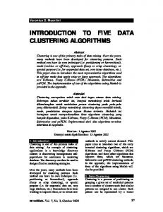
Figure 1: 3–D Plot of the sin(x1 )2 + sin(x2 )2 function The six DE variants described above are applied to compute the global minima of the objective function f . Experimental results indicate that DE1 exhibits very fast convergence to one of the global minima of f . On the contrary, DE2 explores a large portion of the search space before converging to a solution. This fact is illustrated in Figures 2 and 3, where (for visualization purposes) a population consisting of 1000 individuals is plotted after 1, 5, 10, 20 generations of DE1 and DE2 , respectively. A closer look at Equations (1) and (2) reveals that DE1 uses the best individual as a starting point for the computation of the mutant vector, thus constantly pushing the population closer to the location of the best computed point. On

The performance of algorithms DE3 and DE4 resembles that of DE1 , due to the use of the best individual. However, DE3 and DE4 exhibited better exploration than DE1 , since they also incorporate randomly selected individuals. Algorithms DE5 and DE6 use only randomly selected individuals resulting in maximum exploration and the individuals of their populations are simultaneously attracted by more than one minimizers. In Figure 4 the population of the DE6 algorithm at different generations is plotted. Figures 3 and 4 show that some mutation operators have the tendency to concentrate subsets of the population in the region of attraction of different minimizers of the objective function. This observation motivated the incorporation of a clustering algorithm to identify such subsets. Experiments indicate that the k–windows clustering algorithm discovers boxes capturing subpopulations of individuals located in the region of a minimizer. Consequently, the subpopulations are confined to search within each box. Thus, the optimization of the objective function proceeds without affecting the dynamics of the DE algorithm. This process gives all the minima existing in regions that the DE algorithm explored before the use of the clustering operator. It is obvious that DE

4

4

2

2

0

0

-2

-2

-4

-4

-4

-2

0

2

4

4

4

2

2

0

0

-2

-2

-4

-4

-2

0

2

4

-4

-2

0

2

4

-4

-4

-2

0

2

4

Figure 4: DE6 population after 1, 5, 10, and 20 generations algorithm must adequately explore the search space prior to the call of the clustering operator. In the next section, for completeness purposes, we give a brief description of the k–windows clustering algorithm.

3 The Unsupervised k–windows Clustering Algorithm The recently proposed k–windows clustering algorithm uses a windowing technique to discover the clusters present in an n–dimensional dataset. More specifically, assuming that the dataset lies in n dimensions, the algorithm initializes a number of n–dimensional windows (boxes) over the dataset. Subsequently, it iteratively perturbs these windows using the movement and enlargement procedures, in order to capture within each window patterns that belong to a single cluster. The movement and enlargement procedures are guided by the points that lie within each window. As soon as the movement and enlargement procedures do not significantly increase the number of points within each window they terminate. The final set of windows defines the clustering result of the algorithm. A fundamental issue in cluster analysis, independent of the particular clustering technique applied, is the determination of the number of clusters present in a dataset. For instance well–known and widely used iterative techniques, such as the k–means algorithm [12] as well as the fuzzy c– means algorithm [5], require from the user to specify the number of clusters present in the data prior to the execution of the algorithm. On the other hand, the unsupervised k– windows algorithm is capable to determine the number of clusters through a generalization of the original algorithm. The unsupervised version of the k–windows algorithm was used in this paper, since the number of minima of an objective function is, in general, unknown. For a comprehensive description of the algorithm and an investigation of its capability to automatically identify the number of clusters present in a dataset, refer to [3, 4, 32, 36]. It must be noted that no objective function evaluations are necessary during the operation of the k–windows clustering algorithm. The computationally demanding step of

the k–windows clustering algorithm is the determination of the points that lie in a specific window. This is the well studied orthogonal range search problem [23]. Numerous Computational Geometry techniques have been proposed [2, 23] to address this problem. All these techniques employ a preprocessing stage at which they construct a data structure that stores the patterns. This data structure allows them to answer range queries fast. For applications of very high dimensionality, data structures like the Multidimensional Binary Tree [23] are more suitable. On the other hand, for low dimensional data with a large number of points the approach of [2] seems more attractive. The k–windows clustering algorithm has been successfully applied in numerous applications including bioinformatics [33, 34], medical diagnosis [18, 35], and time series prediction [19].

4 The Proposed Clustering Operator In this section, the clustering operator is described. The proposed operator utilizes the unsupervised k–windows algorithm and is called only once, after a user–defined number of generations. In practice, a small number of generations is sufficient for the DE algorithm to explore the search space. Afterwards, the clusters of individuals are determined and subpopulations are confined within each region. Each subpopulation has NP/β individuals, where β is the number of clusters found. If a region contains more individuals, the clustering operator selects the best NP/β. On the other hand, if less individuals exist the clustering operator initializes new ones. The result of the algorithm is the location of many minima in a single run, including the global one. The modified DE algorithm using the clustering operator is outlined in Algorithm 1. D IFFERENTIAL E VOLUTION A LGORITHM M ODEL 0: Initialize the population of NP individuals 1: Evaluate the fitness of each individual 2: Repeat 3: For i = 1 to NP 4: Mutation(xig ) → Mutantig 5: Recombination(Mutantig) → Trialig 6: If f(Trialig ) 6 f (xig ), 7: accept Trialig for the next generation 8: EndFor 9: Until the search space is sufficiently explored 10: Find β clusters using the clustering operator 11: For j = 1 to β 12: Confine NP/β individuals within each cluster 13: Use the DE algorithm to compute the minimum 14: EndFor 15: Return all the computed minima Algorithm 1: The proposed algorithm in pseudocode. To better utilize the proposed approach it is advisable to start the DE algorithm using a mutation operator that permits adequate exploration of the search space (for example DE2 or DE6 ). Once the clusters around the minima have been determined, one can switch to a mutation operator that

has faster convergence speed (for example DE1 ). Note that instead of using again the DE algorithm in Steps 12 and 13 of Algorithm 1, any other minimization algorithm (even not an evolutionary one) can be employed. For very hard optimization problems, when the objective function is defined in many dimensions and possesses multitudes of local and global minima, the clustering operator could be called more than once. The same might be true for real–life optimization tasks, where the function value of the global minimum is unknown. Each consecutive call of the clustering operator will result in more promising subregions of the original search space and will save unneeded objective function evaluations, since the subpopulations will stay focused on regions containing desirable minima. For all the experiments conducted in this paper, one call of the clustering operator was sufficient for the algorithm to locate the global, as well as, many local minima. To determine the applicability and the efficiency of the proposed clustering operator we incorporated it to the DE algorithm and applied the new method to the multimodal test function f , defined in Section 2.2, which posses 9 global minima in the hypercube [−5, 5]2 . The result of the application of the clustering operator on the function f is illustrated in Figure 5. 6

4

DE1 DE2 DE3 DE4 DE5 DE6

Original DE Algorithm DE with k–win Min Mean Max Min Mean Max 54 110.2 203 1 17.5 66 57 119.1 294 1 1.0 1 60 133.0 239 1 1.1 7 52 114.9 212 1 1.0 1 49 106.7 245 1 1.0 1 62 111.4 221 1 1.0 1

Table 1: Restarts needed to locate all the minimizers of f individuals was used and the mutation and recombination constants had values µ = 0.6 and ρ = 0.8, respectively. The algorithm was terminated when the global minimum was located. The proposed clustering operator was called only once for the optimization of each of the four test function considered below, after 20, 20, 10, and 200 generations, respectively. For each test function used, we present a table (Tables 2– 5) summarizing the average results for the 100 runs. The first column of the table indicates the name of the algorithm and the second column the average number of generations needed for the algorithm to locate the global minimum without the use of the clustering operator. The third and fourth columns give the average number of minima discovered (including the global one) and the corresponding average generations needed for the DE algorithm to locate the global minimum using the clustering operator.

2

5.1 The Levy No. 5 Test Function

0

The first test function considered is the Levy No. 5:

-2

f1 (~x) = σ1 σ2 + (x1 + 1.42513)2 + (x2 + 0.80032)2

-4

-6 -6

-4

-2

0

2

4

6

where xi ∈ [−10, 10], i = 1, 2, and σ1 and σ2 are given by:

Figure 5: Clusters and global minimizers discovered in f It must be noted that a number of independent experiments of the original DE algorithm gives no guarantee that all global minimizers will be detected, since the algorithm has no memory; no information concerning previously detected minimizers is kept. We performed 100 independent simulations, using each one of the six different mutation operators described above and Table 1 exhibits the average number of restarts needed for the DE algorithms to locate all the global minimizers of f . The modified algorithm that uses the clustering operator in most cases managed to find all the minimizers of f in a single execution.

5 Experimental Results We implemented and tested the proposed clustering operator on a number of hard optimization tasks and it exhibited stable and robust performance. In this section we report the experimental results from 4 well–known minimization test functions. For each mutation operator we performed 100 independent experiments. A population consisting of 200

σ1 = σ2 =

5 X

i=1 5 X

i cos[(i + 1)x1 + i], j cos[(j + 1)x2 + j].

j=1

There exist about 760 local minima and one global minimum with function value f1∗ = −176.1375 located at ~x∗ = (−1.3068, −1.4248). The large number of local optimizers makes it extremely difficult for any method to locate the global minimizer.

DE1 DE2 DE3 DE4 DE5 DE6

w/o k-win operator with k-win operator Generations Minima located Generations 33.21 5.97 34.36 70.66 20.52 54.26 64.09 11.96 39.77 65.11 20.22 50.25 133.01 22.70 70.85 64.89 19.20 50.24 Table 2: Average results for the Levy function

The experimental results exhibited in Table 2 indicate that generally the use of the clustering operator enhances the performance of the DE algorithms. In detail, there is an average acceleration of the algorithm’s convergence speed ranging from 30% to 80%. Additionally, as many as 20 minima (including the global one) were simultaneously computed. The only exception is DE1 where a slight increase in the generations is observed (3%), but the modified algorithm locates the global as well as 5 local minima. To better demonstrate the ability of the proposed approach to locate many minima at once, independent runs were conducted with the number of individuals in the population gradually increasing from 200 to 2000. In general, a larger population explores better the search space and more regions containing minima are located by the k–windows operator. In Figure 6 we exhibit the detailed results. The algorithm DE1 locates on average 10 minima regardless of the size of its populations. On the contrary, the rest of the algorithms locate more minima as their population is increased. DE5 exhibited the best performance finding simultaneously up to 85 minima.

DE1 DE2 DE3 DE4 DE5 DE6

w/o k-win operator with k-win operator Generations Minima located Generations 20.93 1.00 26.34 61.67 17.19 45.72 80.11 11.23 34.88 47.17 13.89 42.64 98.69 19.43 54.74 55.26 15.72 44.28

Table 3: Average results for the Rastrigin function 5.3 The Shekel’s Foxholes Test Function This is a 2–dimensional test function given by the following equation: 1 f3 (~x) = , 0.002 + ψ(~x) where xi ∈ [−65.536, 65.536], i = 1, 2 and ψ(~x) =

24 X l=0

90 80

Minima Discovered

70

1+l+

i=1 (xi

− ali )6

.

The parameters for this function are:

Strategy 1 Strategy 2 Strategy 3 Strategy 4 Strategy 5 Strategy 6

ak1

60

ak2

50

= {−32, −16, 0, 16, 32}, where k = {0, 1, 2, 3, 4} and ak1 = ak mod 5,1 = {−32, −16, 0, 16, 32}, where

k = {0, 5, 10, 15, 20} and ak2 = ak+m,2 , m = {1, 2, 3, 4}.

40 30 20 10 0 200

1 P2

400

600

800

1000 1200 Population Size

1400

1600

1800

2000

Figure 6: The effect of the population size on the number of located minima for the Levy test function

The global minimum of f1 (−32, −32) = 0.998004. This is a relatively easy test function and was included in the experiments in order to investigate the performance of the clustering operator when applied to problems for which the DE algorithm requires a relatively small number of generations to locate the global minimizer.

5.2 The Rastrigin Test Function The Rastrigin test function is a typical example of a non– linear multimodal function. This function was first proposed by Rastrigin as a 2–dimensional function [38] and is a fairly difficult problem due to its large number of local minima. It is given by the following equation: f2 (~x) =

2 X i=1

x2i − cos(18xi )




where xi ∈ [−1, 1], i = 1, 2. There exist 49 local minima. Table 3 summarizes the average results from the 100 experiments. The results for the Rastrigin function are similar to the results for the Levy function. Faster convergence is exhibited for all the DE algorithms (except DE1 ). The average increase in convergence speed was from 10% to 130% and up to 20 minima were simultaneously located.

DE1 DE2 DE3 DE4 DE5 DE6

w/o k-win operator with k-win operator Generations Minima located Generations 7.70 7.81 12.58 12.95 12.58 13.69 2.04 9.34 12.43 10.75 8.13 12.24 11.86 9.87 16.85 2.76 14.33 13.58

Table 4: Average results for the Shekel’s Foxholes function In Table 4 the average performance of the algorithms is exhibited. It is clear that the use of the clustering operator results in the computation of many minima at once, but the problem is so easy that there is always an increase in the number of generations needed to locate the global minimum. This fact indicates that the proposed approach is better suited to difficult optimization tasks, when more than one minimizer is sought.

5.4 The 10–dimensional Griewangk Test Function This test function is a generalization of the 2–dimensional Griewangk function, which is known to be relatively difficult to minimize and is given by the following equation:   10 10 1 X 2 Y xi x − cos √ + 1, f4 (~x) = 4000 i=1 i i=1 i where xi ∈ [−10, 10], i = 1, 2. This test function is riddled with local minima. The global minimum of the function is f4 (0, . . . , 0) = 0.

DE1 DE2 DE3 DE4 DE5 DE6

w/o k-win operator with k-win operator Generations Minima located Generations 302.34 14.19 415.55 873.93 8.58 346.31 799.06 23.36 439.82 1280.42 4.40 356.52 1816.09 1.65 571.30 619.43 18.09 328.31

Table 5: Average results for the Griewangk function The experimental results illustrated in Table 5 show that the clustering operator greatly accelerates the DE algorithms ranging from 80% to 260%. Again, DE1 is the exception; although on average 14 minima are located the proposed algorithm requires 27% additional generations.

6 Conclusion In this work we propose a novel clustering operator and investigate its impact on the performance of the Differential Evolution optimization algorithm. This operator uses the recently proposed unsupervised k–windows clustering algorithm. The k–windows clustering algorithm uses previously computed pieces of information in an attempt to discover regions containing groups of individuals attracted by different minima. Experiments show that the proposed approach greatly accelerates the convergence speed of the DE algorithms and that in addition to the global minimum is capable to locate simultaneously many local minima without extra function evaluations. To this end, the use of the proposed clustering operator is always suggested. In brief, the clustering operator has the following advantages: 1. locates local minima with relatively low function value, in addition to the global ones, 2. in general, fewer generations are required for the DE algorithm to converge, 3. there is no need for additional function evaluations, 4. utilizes the range search algorithm for fast and reliable execution, 5. its parallel implementation is straightforward [7], 6. is better suited to difficult high–dimensional multimodal objective functions. In a future correspondence, we will present an adaptive scheme, based on the average movement of each individual, for the automatic call of the clustering operator. This

scheme will ensure that the search space is sufficiently explored. We also intend to investigate the parallel implementation of the proposed approach, as well as its performance on difficult high–dimensional real–life problems encountered in bioinformatics, medical applications and neural network training.

Acknowledgment The authors would like to thank the referees for their constructive comments and useful suggestions that helped to improve this paper. We also thank the European Social Fund, Operational Program for Educational and Vocational Training II (EPEAEK II), and particularly the Program “Pythagoras” for funding this work. This work was also partially supported by the University of Patras Research Committee through a “Karatheodoris” research grant.

Bibliography [1] M. S. Aldenderfer and R. K. Blashfield. Cluster Analysis, volume 44 of Quantitative Applications in the Social Sciences. SAGE Publications, London, 1984. [2] P. Alevizos. An algorithm for orthogonal range search in d > 3 dimensions. In Proceedings of the 14th European Workshop on Computational Geometry. Barcelona, 1998. [3] P. Alevizos, B. Boutsinas, D.K. Tasoulis, and M.N. Vrahatis. Improving the orthogonal range search kwindows clustering algorithm. In Proceedings of the 14th IEEE International Conference on Tools with Artificial Intelligence, pages 239–245. Washington, D.C., 2002. [4] P. Alevizos, D.K. Tasoulis, and M.N. Vrahatis. Parallelizing the unsupervised k-windows clustering algorithm. In R. Wyrzykowski, editor, Lecture Notes in Computer Science, volume 3019, pages 225–232. Springer-Verlag, 2004. [5] J.C. Bezdek. Pattern Recognition with Fuzzy Objective Function Algorithms. Kluwer Academic Publishers, 1981. [6] M.R. DiSilvestro and J.-K.F. Suh. A cross-validation of the biphasic poroviscoelastic model of articular cartilage in unconfined compression, indentation, and confined compression. Journal of Biomechanics, 34:519–525, 2001. [7] V.P. Plagianakos D.K. Tasoulis, N.G. Pavlidis and M.N. Vrahatis. Parallel differential evolution. In IEEE Congress on Evolutionary Computation (CEC 2004), 2004. [8] H.Y. Fan and J. Lampinen. A trigonometric mutation operation to differential evolution. Journal of Global Optimization, 27:105–129, 2003. [9] D. Fogel. Evolutionary Computation: Towards a New Philosophy of Machine Intelligence. IEEE Press, Piscataway, NJ, 1996. [10] L.J. Fogel, A.J. Owens, and M.J. Walsh. Artificial intelligence through simulated evolution. Wiley, 1966.

[11] D. Goldberg. Genetic Algorithms in Search, Optimization, and Machine Learning. Addison Wesley, Reading, MA, 1989. [12] J. A. Hartigan and M. A. Wong. A k-means clustering algorithm. Applied Statistics, 28:100–108, 1979. [13] J.H. Holland. Adaptation in natural and artificial system. University of Michigan Press, 1975. [14] J. Hou, P.H. Siegel, and L.B. Milstein. Performance analysis and code optimization of low density paritycheck codes on rayleigh fading channels. IEEE Journal on Selected Areas in Communications, 19:924– 934, 2001. [15] J. Ilonen, J.-K. Kamarainen, and J. Lampinen. Differential evolution training algorithm for feed forward neural networks. Neural Processing Letters, 17(1):93– 105, 2003. [16] J.R. Koza. Genetic Programming: On the Programming of Computers by Means of Natural Selection. MIT Press, 1992. [17] C. Linnaeus. Clavis Classium in Systemate Phytologorum in Bibliotheca Botanica. Amsterdam, The Netherlands: Biblioteca Botanica, 1736. [18] G.D. Magoulas, V.P. Plagianakos, D.K. Tasoulis, and M.N. Vrahatis. Tumor detection in colonoscopy using the unsupervised k–windows clustering algorithm and neural networks. In Fourth European Symposium on “Biomedical Engineering”, 2004. [19] N.G. Pavlidis, D.K. Tasoulis, and M.N. Vrahatis. Financial forecasting through unsupervised clustering and evolutionary trained neural networks. In Congress on Evolutionary Computation, Canberra Australia, 2003. [20] V.P. Plagianakos and M.N. Vrahatis. Neural network training with constrained integer weights. In P.J. Angeline, Z. Michalewicz, M. Schoenauer, X. Yao, and A. Zalzala, editors, Proceedings of the Congress of Evolutionary Computation (CEC’99), pages 2007– 2013. IEEE Press, 1999. [21] V.P. Plagianakos and M.N. Vrahatis. Training neural networks with 3–bit integer weights. In W. Banzhaf, J. Daida, A.E. Eiben, M.H. Garzon, V. Honavar, M. Jakiela, and R.E. Smith, editors, Proceedings of the Genetic and Evolutionary Computation Conference (GECCO’99), pages 910–915. Morgan Kaufmann, 1999. [22] V.P. Plagianakos and M.N. Vrahatis. Parallel evolutionary training algorithms for ‘hardware-friendly’ neural networks. Natural Computing, 1:307–322, 2002. [23] F. Preparata and M. Shamos. Computational Geometry. Springer Verlag, New York, Berlin, 1985. [24] V. Ramasubramanian and K. Paliwal. Fast kdimensional tree algorithms for nearest neighbor search with application to vector quantization encoding. IEEE Transactions on Signal Processing, 40(3):518–531, 1992. [25] I. Rechenberg. Evolution strategy. In J.M. Zurada, R.J. Marks II, and C. Robinson, editors, Computational Intelligence: Imitating Life. IEEE Press, Piscataway, NJ, 1994.

[26] T.J. Richardson, M.A. Shokrollahi, and R.L. Urbanke. Design of capacity-approaching irregular low-density parity-check codes. IEEE Transactions on Information Theory, 47:619–637, 2001. [27] H.-P. Schwefel. Evolution and Optimum Seeking. Wiley, New York, 1995. [28] R. Storn. Differential evolution design of an iir-filter. In IEEE International Conference on Evolutionary Computation ICEC’96, 1996. [29] R. Storn. System design by constraint adaptation and differential evolution. IEEE Transactions on Evolutionary Computation, 3:22–34, 1999. [30] R. Storn and K. Price. Minimizing the real functions of the icec’96 contest by differential evolution. In IEEE Conference on Evolutionary Computation, pages 842– 844, 1996. [31] R. Storn and K. Price. Differential evolution – a simple and efficient adaptive scheme for global optimization over continuous spaces. Journal of Global Optimization, 11:341–359, 1997. [32] D.K. Tasoulis, P. Alevizos, B. Boutsinas, and M.N. Vrahatis. Parallel unsupervised k-windows: an efficient parallel clustering algorithm. In V. Malyshkin, editor, Lecture Notes in Computer Science, volume 2763, pages 336–344. Springer-Verlag, 2003. [33] D.K. Tasoulis, V.P. Plagianakos, and M.N. Vrahatis. Unsupervised cluster analysis in bioinformatics. In Fourth European Symposium on “Biomedical Engineering”, 2004. [34] D.K. Tasoulis, V.P. Plagianakos, and M.N. Vrahatis. Unsupervised clustering of bioinformatics data. In European Symposium on Intelligent Technologies, Hybrid Systems and their implementation on Smart Adaptive Systems, Eunite, pages 47–53, 2004. [35] D.K. Tasoulis, L. Vladutu, V.P. Plagianakos, A. Bezerianos, and M.N. Vrahatis. On-line neural network training for automatic ischemia episode detection. In Leszek Rutkowski, J¨org H. Siekmann, Ryszard Tadeusiewicz, and Lotfi A. Zadeh, editors, Lecture Notes in Computer Science, volume 2070, pages 1062–1068. Springer-Verlag, 2003. [36] D.K. Tasoulis and M.N. Vrahatis. Unsupervised distributed clustering. In IASTED International Conference on Parallel and Distributed Computing and Networks, pages 347–351. Innsbruck, Austria, 2004. [37] G.T. Timmer. Global optimization - A stochastic approach. PhD thesis, Erasmus University Rotterdam, 1994. ˇ [38] A.A. T¨orn and A. Zilinskas. Global Optimization. Springer-Verlag, Berlin, 1989. [39] A.A. T¨orn. Cluster analysis as a tool in a global optimization model. In Third International Congress of Cybernetics and Systems, Bucharest, pages 249–260. Springer Verlag, 1977. [40] A.A. T¨orn. Cluster analysis using seed points and density-determined hyperspheres with an application to global optimization. IEEE trans. on Systems, Man and Cybernetics, 7:610–616, 1977. [41] C. Tryon. Cluster Analysis. Ann Arbor, MI: Edward Brothers, 1939.