Clustering of Pre-Main Sequence Stars in the Orion ... - CiteSeerX

{1{

Clustering of Pre-Main Sequence Stars in the Orion, Ophiuchus, Chamaeleon, Vela, and Lupus Star Forming Regions

Yasushi Nakajima

Department of Astrophysics Nagoya University November 1997

{2{ ACKNOWLEDGEMENT

I thank Tomoyuki Hanawa for his supervision. I thank Makoto Nakano and Kengo Tachihara for their collaboration for the work of which manuscript has been accepted by the Astrophysical Journal. I thank Yasuo Fukui, Satoru Ikeuchi, Tomoo Nagahama, and Ken'ichi Tatematsu for their useful discussions, comments, and advice. I also thank anonymous referee of the Astrophysical Journal for the recommendation on discussion on the eects of extinction. Also I thank all my friends and parents for helping and encouraging me in various aspects throughout this work.

{3{ ABSTRACT

Stars have been studied for a long time as the elementary component of the Universe. Chandrasekhar (1958) summarized the structure of main sequence stars in his book. Hayashi, Hoshi, & Sugimoto (1962) summarized stellar evolution in their review paper. However, there are a lot of problems yet to be solved on the birth of stars. It was only recently that a standard scenario of an isolated single star formation has emerged. Although the majority of stars are formed in clusters, properties of stars as cluster still remains to be less studied than single star formation. In this paper, I therefore study the distribution of young stars in nearby star forming regions and discuss their properties as clusters. Larson [MNRAS, 272, 213, (1995)] was one of the most aective studies on clustering of young stars. Larson (1995) calculated the average surface density of companions as a function of angular distance using published data. The average surface density of companions is a kind of two-point correlation function. Larson (1995) showed that the average surface density of companions, 6(), can be tted by two distinct power-law functions [6() /  ] at large and small separations, . Larson (1995) considered that the power-law at small separations represents the distribution of binary separation and that at large separations represents the hierarchical structure of parent cloud. Then he claimed that the position of the intersection of the two power-law (the break of the power-law) represents the intrinsic scale in star formation process. The position is at a separation of 0.04 pc, which coincides with the typical size of molecular cloud core. Larson (1995) considered it supports his claim. Larson (1995)'s claim received much attention. However, his claim was obtained solely from the Taurus star forming region with a single statistical method. To obtain a universal conclusion, it is necessary to compare plural regions with plural statistical methods. Thus I study all the major nearby star forming regions; the Orion, Ophiuchus, Chamaeleon, Vela, and Lupus. I exploit published data. I obtain the average surface density of companions as Larson (1995) did. Also I obtain the distribution of the nearest neighbor distance to study a dierent aspect of the characteristic of distributions. In most of the regions studied, the function can be tted by two power laws (6 /  ) with a break as found by Larson (1995) for the Taurus star forming region. The position of the break is dierent from region to region. It is located around 0.01 - 0.1 pc. The average surface density of companions at smaller separations than the break depends strongly on the separations. The power index does not show signi cant dierence from region to region (  02). The average surface density of companions at larger separations than the break depends weakly on the separations. The power index shows signi cant variation from region to region (00:8 < < 00:1).

{4{ The distribution of the nearest-neighbor distance is represented by the Poisson distribution or distributions broader than that. The power index at the large separations correlates to the distribution of the nearest-neighbor distance. When the latter is tted by the Poisson distribution, the power index is close to 0. When the latter is broader than the Poisson distribution, the power index is negatively large. The broad distribution of the nearest-neighbor distance can be interpreted as the result of superposition of the Poisson distributions of dierent surface density. The power-law t therefore originates from the variation in the surface density within the region. Numerical simulations show that the average surface density of companions is tted by power-law if the region contains several stellar groups of dierent surface densities. At the same time the numerical simulations reproduce the distributions of the nearest-neighbor distance for the observed stars. The power index does not depend on the arrangement of the clusters. The density distribution need not to be hierarchical to explain the observed power-law in the average surface density of companions. There is a clear correlation between the break in the average surface density of companions and the distribution of the nearest neighbor distance. When the average surface density of companions has a break, the nearest neighbor distribution has another component at small separations. The component depends weakly on  and is dominant only at small separations. The position of the break appears where the two components of the nearest neighbor distribution meet. The position of the break is about one tenth of the mean of the distribution of the nearest neighbor distance. Analyses in this paper suggest that the power-law t may indicate star formation history in the region. Because of the velocity dispersion, stars move from the birthplaces and the surface density of coeval stars decreases with the age. If stars are formed at dierent epochs, star forming region contains several groups of dierent surface density. The average surface density of companions will be tted by power-law function and the power index is expected to depend on the history of star formation. I will comment on the work of Larson (1995) as follows. It is universal that the surface distribution can be tted by a combination of two power-law functions. The power-law t, however, originates not from a hierarchical structure but from the stellar density variations in a star forming region. The position of the break in the average surface companion density is not an intrinsic scale in star formation process.

Contents

1 Review on clustering of pre-main sequence stars

1 2

3

INTRODUCTION : : : : : : : : : : : : : : : : : : : : : : : : : : : : : : PRE-MAIN SEQUENCE STAR : : : : : : : : : : : : : : : : : : : : : : : 2.1 Observational features : : : : : : : : : : : : : : : : : : : : : : : : 2.1.1 T Tauri stars : : : : : : : : : : : : : : : : : : : : : : : : 2.1.2 Herbig Ae/Be stars : : : : : : : : : : : : : : : : : : : : : 2.1.3 Protostars : : : : : : : : : : : : : : : : : : : : : : : : : : 2.2 Physical quantities : : : : : : : : : : : : : : : : : : : : : : : : : : 2.2.1 Age : : : : : : : : : : : : : : : : : : : : : : : : : : : : : 2.2.1.1 Age determination based on the HR diagram 15 2.2.1.2 Age detemination based on a statistical method 17 2.2.2 Luminosity and Temperature : : : : : : : : : : : : : : : 2.3 Classi cation based on spectral energy distribution : : : : : : : : 2.3.1 Based on infrared wavelengths : : : : : : : : : : : : : : : 2.3.2 Based on millimeter wavelength : : : : : : : : : : : : : : PRE-MAIN SEQUENCE STAR SURVEYS : : : : : : : : : : : : : : : : 3.1 Techniques : : : : : : : : : : : : : : : : : : : : : : : : : : : : : : : 5

9 : : : : : : : : : : : : : : : :

: : : : : : : : : : : :

9 10 10 11 13 14 15 15

17 18 18 20 21 21

{6{

4

5

3.1.1 Radio continuum survey : : : : : : : : : : : : : 3.1.2 2.6 mm CO line survey : : : : : : : : : : : : : : 3.1.3 Far-infrared survey : : : : : : : : : : : : : : : : 3.1.4 Near-infrared survey : : : : : : : : : : : : : : : 3.1.5 Optical objective prism survey : : : : : : : : : 3.1.6 Optical proper motion survey : : : : : : : : : : 3.1.7 X-ray survey : : : : : : : : : : : : : : : : : : : 3.1.8 Binary survey : : : : : : : : : : : : : : : : : : : 3.2 Individual regions : : : : : : : : : : : : : : : : : : : : : : 3.2.1 Taurus : : : : : : : : : : : : : : : : : : : : : : : 3.2.2 Orion : : : : : : : : : : : : : : : : : : : : : : : 3.2.3  Ophiuchus : : : : : : : : : : : : : : : : : : : 3.2.4 Chamaeleon : : : : : : : : : : : : : : : : : : : : 3.2.5 Lupus : : : : : : : : : : : : : : : : : : : : : : : 3.2.6 Vela : : : : : : : : : : : : : : : : : : : : : : : : 3.2.7 R Coronae Australis : : : : : : : : : : : : : : : CHARACTERISTICS AS GROUPS : : : : : : : : : : : : : : : 4.1 Spatial Distribution : : : : : : : : : : : : : : : : : : : : : 4.1.1 Isolated and clustered modes of star formation : 4.1.2 Widespread WTTS : : : : : : : : : : : : : : : : 4.1.3 Multiplicity of pre-main sequence star : : : : : 4.2 Temporal Properties : : : : : : : : : : : : : : : : : : : : 4.2.1 Dispersal of Pre-Main Sequence Stars : : : : : : 4.2.2 Star Formation History : : : : : : : : : : : : : STATISTICAL STUDIES ON CLUSTERING : : : : : : : : : : 5.1 The two-point correlation : : : : : : : : : : : : : : : : :

:: : : : :: : : :: : : : : : :: : : : : : : :: : : : : : :: : : : : :: : : : : : :: : : : : : : : :: : : : : :: : : : : : : :: : :: : : : :: : :: : : : : : : : : :: : : : : : :: : : : :: : : : : : :: : : : : : : : :: : : : :: : : : : : : : :: : : : :: : : : : : : : :: : : : : : :: : : : : :: : : : : : : :: : : : : : :: : : :: : : : :

21 22 22 24 26 28 28 29 29 29 33 37 40 42 43 46 47 47 47 49 50 51 52 52 53 53

{7{ 5.2 5.3

Nearest-neighbor distribution Stellar density enhancement :

: :: : : : :: : : : :: : : : : :: : : : : : : : : :: : : : :: : : : :: : : : ::

56 57

2 Statistical Analyses on Clustering of Pre-Main Sequence Stars in the Orion, Ophiuchus, Chamaeleon, Vela, and Lupus Star Forming Regions 61

1 2

3 4

5

INTRODUCTION : : : : : : : : : : : : : : : : : : : : : : DATA SAMPLING : : : : : : : : : : : : : : : : : : : : : : 2.1 Orion : : : : : : : : : : : : : : : : : : : : : : : : : 2.2 Ophiuchus : : : : : : : : : : : : : : : : : : : : : : : 2.3 Chamaeleon : : : : : : : : : : : : : : : : : : : : : : 2.4 Vela : : : : : : : : : : : : : : : : : : : : : : : : : : 2.5 Lupus : : : : : : : : : : : : : : : : : : : : : : : : : CALCULATION OF ASDEC : : : : : : : : : : : : : : : : RESULTS : : : : : : : : : : : : : : : : : : : : : : : : : : : 4.1 Orion OB : : : : : : : : : : : : : : : : : : : : : : : 4.2 Orion A : : : : : : : : : : : : : : : : : : : : : : : : 4.3 Orion B : : : : : : : : : : : : : : : : : : : : : : : : 4.4 Ophiuchus : : : : : : : : : : : : : : : : : : : : : : : 4.5 Chamaeleon : : : : : : : : : : : : : : : : : : : : : : 4.6 Vela : : : : : : : : : : : : : : : : : : : : : : : : : : 4.7 Lupus : : : : : : : : : : : : : : : : : : : : : : : : : 4.8 Comparison of Star Forming Regions : : : : : : : : DISCUSSION : : : : : : : : : : : : : : : : : : : : : : : : : 5.1 The Origin of the Power-Law at Large Separations 5.1.1 Spatial Distribution : : : : : : : : : : : : 5.1.2 Eect of Extinction : : : : : : : : : : : :

: : : : :: : : : : : : : : :: : : : : : : : : : :: : : : : :: : : : :: : : : : : : :: : : : : : : :: : : : :: : : : : : :: : : : : : : : :: : : : :: : : :: : : : :: : : :: : : : :: : : : : : : : :: : : : : : : : : :: : : : : :: : : : :: : : : : : : :: : : : : : : :: : : : :: : : : : : :: : : : : : : : : :: : : : : : : : :: : : : :: : : :: : : : :: : : : : :: : : : : : : :: : : : :: : :

61 62 62 64 64 65 65 65 66 66 69 70 72 74 75 75 76 77 78 78 81

{8{ 5.1.3 Age Eect : : : : : : : : : : : : : : 5.2 Binary Frequency : : : : : : : : : : : : : : : 5.3 The Origin of the Break in ASDEC : : : : : 6 CONCLUSION : : : : : : : : : : : : : : : : : : : : A QUALITY OF THE SAMPLES : : : : : : : : : : : A.1 Incompleteness : : : : : : : : : : : : : : : : A.1.1 Magnitude Limit : : : : : : : : : : A.1.2 Absence of X-ray survey : : : : : : A.1.3 Angular Resolution : : : : : : : : : A.1.4 Variability of emission-line : : : : : A.2 Background and Foreground Contamination

: :: : : : :: : : : :: : : : : :: : : : :: : : : : : : :: : : : : :: : : : : : :: : : : :: : : : :: : :: : : : : :: : : : :: : : : :: : : : :: : : : : : :: : : : : :: : : : :: : : : :: : : : :: : : : :: : : : : :: : : : :: : : : : : : :: : : : : :: : : : :: : : : :: : : : : :: :

82 83 84 84 85 86 86 87 87 88 88

Chapter 1

Review on clustering of pre-main sequence stars

1. INTRODUCTION

Understanding of stars is essential in astronomy. Stars are the elementary component of the Universe. Properties of stars are often basic to study other astronomical objects such as galaxies. Stars have been studied for a long time. Chandrasekhar (1958) summarized the structure of main sequence stars in his book. Hayashi, Hoshi, & Sugimoto (1962) summarized stellar evolution in their review paper. However, there are a lot of problems yet to be solved on the birth of stars. It was only recently that a standard scenario of an isolated single star formation has emerged (e.g., Shu, Adams, & Lizano 1987). In the scenario, the problem was simpli ed to extract essential points by neglecting outer environmental eects such as radiation and stellar wind from nearby stars. Observations have shown that the majority of stars are formed in cluster. Thus the formation mechanism is likely to be governed by cluster environment for the majority of the stars. However, star formation in cluster still remains to be much less studied than single star formation. Clustering in star formation is therefore an important issue to be solved. Statistical methods are useful in studying clustering of young stars. Recent statistical work by Larson (1995) gave an insight into the star formation in cluster and received much attention. Larson (1995) derived \the intrinsic scale of star formation mechanism" from the distribution of young stars in the Taurus star forming region. Also he claimed the surface density structure of the young stars inherits the hierarchical structure of the parent 9

{ 10 { molecular clouds. Although the conclusion was aective, it was derived from a single star forming region with a single statistical method. It is not clear whether the conclusion is universal or not. In this paper, I therefore study the distribution of young stars in all the major nearby star forming regions with plural statistical methods and discuss their characteristics as clusters. In this chapter, I review existing studies of clustering of pre-main sequence stars. I begin with current status of studies of pre-main sequence stars as individual objects. In x2, observational features, physical quantities, and classi cation schemes are reviewed. Pre-main sequence stars have been surveyed by exploiting their observational properties. In x3, I summarize existing surveys of pre-main sequence stars in major star forming regions. Surveys have revealed pre-main sequence stars are associated with molecular cloud. In x4, I review current knowledge on the characteristics of pre-main sequence stars as groups. Statistical analyses have revealed clustering nature of pre-main sequence stars. In x5, I review previous works on statistical analyses of clustering of pre-main sequence stars. 2. PRE-MAIN SEQUENCE STAR

Pre-main sequence stars are characterized by their observational appearance. I describe observational features of pre-main sequence stars in x2.1. Physical quantities; age, luminosity, and temperature, for pre-main sequence stars are described in x2.2. I concentrate especially on the age determination. Based on the observational features, pre-main sequence stars are classi ed into several age groups. Pre-main sequence stars are classi ed based on spectral energy distribution at infrared to millimeter wavelengths. I describe the classi cation in x2.3. 2.1. Observational features

While a main sequence star radiates its energy by burning hydrogen, a pre-main sequence star, by de nition, does it by contracting and then releasing gravitational energy. Stars are born during the collapse of gas and dust clouds. As the youngest stars are surrounded by dusty envelope, they are highly extinct at optical wavelength and best observed at infrared and millimeter wavelengths. As the stars evolve, the circumstellar envelopes clear, and the central stars become optically visible. Optically visible low-mass pre-main sequence stars are called T Tauri stars, and intermediate-mass, spectral type earlier than A (or early F), pre-main sequence stars are called Herbig Ae/Be stars. Optically

{ 11 { invisible sources are often called protostars. Visible pre-main sequence stars are distinct from invisible ones by historical and practical reasons. When pre-main sequence stars were discovered as T Tauri stars, we could observe them only at optical wavelengths. Thus only the visible pre-main sequence stars were observed and classi ed in early studies. Even in these days we have less information on invisible pre-main sequence stars than on visible pre-main sequence stars. Invisible pre-main sequence stars are embedded in dense gas and we observe the stellar surface only indirectly. On the other hand, the stellar surface of a visible pre-main sequence star can be measured from its position on the Hertzsprung-Russell (HR) diagram. I review the observational features of T Tauri stars, Herbig Ae/Be stars, and protostars in the followings. 2.1.1. T Tauri stars

T Tauri stars were rst recognized as a separate class of stars by Joy (1945), and soon afterwards Ambartsumian (1947) postulated that T Tauri stars are recently formed, i.e., very young stars. In these days, it is widely accepted that T Tauri stars are pre-main sequence stars. Evidence and suggestion for youth of T Tauri stars are following.  Li I 6707 absorption is observed. The abundance of Lithium decreases with age. It is thought to be destroyed when convective mixing brings it in contact with high-temperature zones.  The positions of T Tauri stars in the HR diagram and comparison with theoretical evolutionary tracks provide further indirect evidence for their youth (Cohen & Kuhi 1979).  T-associations (groups of T Tauri stars) are often found in connection with groups of OB stars (OB-associations). Ambartsumian (1947) postulated that T Tauri stars were the low-mass counterpart of the short-lived (i.e., recently formed) OB stars. Optical spectroscopic properties, or rather de nitions, of T Tauri stars are the following.  Hydrogen Balmer, Ca II H and K lines are observed as emission. One with the equivalent width of H emission-line broader than 10 A is called a classical T Tauri star (CTTS), and narrower than 10 A is called a weak-lined T Tauri star (WTTS).

{ 12 {  Anomalous emission line of Fe I is often, not all, observed.  Forbidden emission lines of [O I] and [S II] are often observed for CTTSs. About 30 % of all T Tauri stars show strong forbidden emission lines, e.g., [O I] 6300, 6363 and [S II]  6716, 6731 lines, with a large equivalent width of W([O I]6300) > 1 A. These lines are expected to be formed by internal shocks within the out ow (Hirth, Mundt, & Solf 1996).  Li I 6707 absorption is strong.  Spectral type is later than F.  A majority of them display Type III P Cygni pro les at H; in these pro les the emission is broad (FWHM  200 km s01) and symmetric, and a blue shifted absorption feature at typically 80 km s01 is superposed on the emission.  They show variability in magnitude, typically 1-2 mag.  Kinetic association with dark cloud has been shown by proper motion and radial velocity studies (Herbig 1977; Jones & Herbig 1979)

As techniques at other wavelengths were developed, T Tauri stars became able to be investigated in wavelengths from X-ray to infrared. Other non-optical properties are the following.  The spectral energy distribution displays ultraviolet excesses. The ultraviolet line uxes are 104-106 times stronger than in the Sun.  The spectral energy distribution displays infrared excesses. Most of its energy is released in the near-infrared wavelengths.  X-ray emission is detected. The most powerful observed X-ray are released 1032 erg s01 which is larger by a factor of 105 than the strongest X-ray solar are (Montmerle et al. 1983).

Improved observational techniques revealed the morphology of the circumstellar environment. High resolution direct imaging at radio, near-infrared, and optical wavelengths revealed circumstellar environment of some T Tauri stars. Envelopes and disks, with sizes of several hundred to several thousand AU, were observed toward, for example, HL Tau (e.g., Hayashi, Ohashi, & Miyama 1993), R Mon (e.g., Sargent & Beckwith 1987), DG Tau (e.g., Ohashi et al. 1991), GG Tau (e.g., Dutrey, Guilloteau & Simon 1994), DL

{ 13 { Tau (e.g., Ohashi et al. 1991), and DM Tau (Saito et al. 1995). Out ow was observed for HL Tau (Ray et al. 1996). Structures of a T Tauri star inferred from the observational properties are following.  Central star has eective temperature of 4000 K.  It is surrounded by dusty accretion disk.  There is boundary layer between the central star and disk, whose temperature is  104 K.  It is associated with stellar wind and some with collimated jets. 2.1.2. Herbig Ae/Be stars

Herbig Ae/Be stars are rst recognized by Herbig (1960). He conjectured that the \Be and Ae stars associated with nebulosity" were objects of intermediate mass still in their pre-main sequence stage of evolution. In fact Herbig Ae/Be stars are pre-main sequence stars of intermediate-mass (2 - 10 M ). In the years since their discovery, their pre-main sequence nature has been amply con rmed. Strom et al. (1972) used surface gravity measurements to show that the radii of selected stars were indeed larger than those of main sequence. Finkenzeller & Jankovics (1984) employed radial velocities to verify the stars' kinematic link to nearby molecular cloud gas. The following are de nitions for the Herbig Ae/Be stars in Catala (1989), although the de nitions are slightly dierent among authors.  The spectral type is earlier than F0: this criterion allows to select only massive objects.  They exhibit emission lines in their spectra: the presence of emission lines was known to be a characteristic of T Tauri stars, and therefore was considered as a criterion of youth.  They lie in an obscured region: another criterion of youth; young stars have not had enough time to escape from their parental clouds.  They illuminate a bright re ection nebula in their immediate vicinity: this criterion eliminates those stars that would simply be projected on dark clouds on the celestial sphere.

{ 14 { van den Ancker, de Winter, & Tjin A Djie (1998) added criteria that Herbig Ae/Be stars have luminosity class III - V and exhibit infrared emission due to circumstellar dust, and excluded the third and forth de nitions by Catala (1989). Some authors also include stars without strong emission lines in samples of Herbig Ae/Be stars (Malfait, Bogaert, & Wealkens 1998). Herbig Ae/Be stars have common spectroscopic and photometric properties with T Tauri stars. However, these two classes of objects have some dierences. Herbig Ae/Be stars generally show a greater dispersion in the observed properties with respect to the more homogeneity exhibited by T Tauri stars (Herbig 1960). Projected rotation velocities (v sin i) are greater than those of T Tauri stars (Finkenzeller 1985). In contrast to the T Tauri stars, the Herbig Ae/Be stars do not show substantial variations (Herbst, Holtzman, & Phelps 1982). 2.1.3. Protostars

A protostar is de ned as a stellar object in the process of assembling the bulk of the material it will contain when it ultimately reaches the main sequence (e.g., Andre, Ward-Thompson, & Barsony 1993). Such objects are expected to be surrounded by dusty envelope and therefore highly extinct at optical wavelength. Consequently, a protostar is expected to be best observed at infrared and millimeter wavelengths. Embedded infrared or submillimeter point sources are candidates for protostars. All optically invisible sources is not protostars, although they are often called protostars conventionally. T Tauri stars are also optically invisible if they are extinct by foreground dusty cloud. Spectral energy distribution at wavelengths from infrared to millimeter is used to select \genuine" protostars. Protostars should be more luminous at longer infrared wavelength. This selection method will be described in x2.3. Besides the characteristic in spectral energy distribution, protostars are characterized by two kinematical features; infall and out ow motions. By de nition, a protostar should present infall motion of gas as observational features. Recent millimeter-wavelength observations have increased the evidence for infall motion onto young stellar objects. The main procedure is to observe spectral lines that trace high densities (n > 104cm03) and have red-shifted self-absorption spatially concentrated around an embedded young stellar object. Sixteen spectroscopic infall candidates were identi ed so far (e.g., Mardones et al. 1997 and references therein).

{ 15 { Some embedded sources are associated with hypersonic out ows, such as Herbig-Haro objects and molecular out ows. The out ows are almost always coincident with, if not centered on, the position of an embedded infrared source. It is widely recognized that the birth of a low-mass star is often rst signalled by a powerful jet and out ow from a deeply embedded object. 2.2. Physical quantities

I review the determinations of physical quantities; age, luminosity, and temperature of pre-main sequence stars in this subsection. Age of a pre-main sequence star is essential for the evolutionary status of the star. I describe the age determination in x2.2.1. I brie y describe the determinations of luminosity and temperature in x2.2.2. 2.2.1. Age

There are two methods to estimate the age of a pre-main sequence star. One is based on its position the HR diagram. This method is applicable for a object of which eective temperature and luminosity can be derived observationally. The other is based on statistics. This method has often been applied for an optically invisible source, of which eective temperature and luminosity are dicult or impossible to be obtained. Age determination based on the HR diagram is summarized in x2.2.1.1 and that based on a statistical method in x2.2.1.2. 2.2.1.1. Age determination based on the HR diagram

Age of an pre-main sequence star is estimated by comparison of theoretical models with the observation on the HR diagram. The evolution of a star from its birth to the main sequence is summarized as follows. A star begins its life as a cold protostar. Accretion of gas onto the star increases the radius and luminosity. As far as the star is embedded in the accreting gas, the star is not optically visible. When the accreting gas becomes transparent, the star is \born" as an optical source. At the \birth", the star has a low surface temperature and high luminosity. Hence the star has a large radius, typically tens solar radii. High mass pre-main sequence stars contracts towards the main sequence while keeping the luminosity almost constant. This contraction on the HR diagram is called the Henyey track. On the other hand, very low mass stars contract keeping the surface temperature almost constant. This contraction is called the Hayashi track. Moderately low

{ 16 {

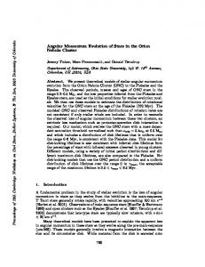
Fig. 1.| HR diagrams for WTTSs detected by ROSAT in the Chamaeleon and Orion star forming regions. The pre-main sequence evolutionary tracks are from D'antona & Mazzitelli (1994), derived for Alexander opacities and with the Canuto and Mazzitelii convection calculation. (Taken from Alcala et al. 1996a)

{ 17 { mass stars contract rst along the Hayashi track and later along the Henyey track. The evolutionary track of a star on the HR diagram depends solely on the mass. It does not intersect with that of a star having another mass on the HR diagram. The position of a pre-main sequence star on the HR diagram tells us the mass and age uniquely (see Figure 1). The theoretical tracks of pre-main sequence stars depend on the assumed opacity law, mixing length theory, and rotation of the star (Mazzitelli 1989). Theoretical models have been improved gradually. Frequently cited models are those of Iben (1965), Grossman & Graboske (1971), Swenson, Stringfellow, & Faulkner (1990), Burrows et al. (1993), and D'Antona & Mazzitelli (1994). In these several years D'Antona & Mazzitelli (1994) is referenced most often for the age determination (e.g., Kenyon & Hartmann 1995). 2.2.1.2. Age detemination based on a statistical method

For optically invisible sources, a statistical method has often been used to derive their lifetimes. In the statistical method, star formation rate is assumed to be constant. Then the abundance of objects at each stage is proportional to that of the lifetime of each stage. Wilking, Lada, & Young (1989) estimated the lifetime of Class I sources (A Class I source is a protostar candidate. See x2.3 for detail.) to be 1-42105 yr from the abundance ratio of Class I sources to T Tauri stars in the  Ophiuchi core. Onishi (1996) estimated that lifetime is roughly 105 yr for cold IRAS sources (protostar candidates) in Taurus from the ratio of the cold IRAS sources to T Tauri stars, 1:10. In his estimation the median age of the T Tauri stars is assumed to be 106 yr in Taurus. Andre & Montmerle (1994) estimated that the lifetime is 5 2103 or 104 yr for Class 0 (See x2.3.) sources in the  Ophiuchi core from the abundance ratio of Class 0 sources to Class I sources. In their estimation the typical lifetime for Class I sources is assumed to be 105 yr. 2.2.2. Luminosity and Temperature

Stellar luminosity is estimated from the ux at I (0.8 m) or J (1.25 m) (J is preferred) after reddening and bolometric corrections (e.g., Hartigan, Strom, & Strom 1994). Usually reddening is evaluated by the V 0 R color excess. Bolometric correction is used to convert an absolute magnitude at J or I to the stellar luminosity and it depends on the spectral type of the star. The ux at the wavelength shorter than I is not used to derive the stellar luminosity since it is contaminated by emission from the boundary layer. The contamination is not serious at the wavelength larger than I . Also the ux at the wavelength longer than J is not used because it is contaminated by emission from circumstellar dust. The optical

{ 18 { and near-infrared excesses in young stars contribute the smallest fraction to the total ux at the wavelengths of I and J (Kenyon & Hartmann 1990; Strom et al. 1988). Eective temperatures can be obtained from observed spectral types of stars (e.g., Hartigan, Strom, & Strom 1994). The spectral types of late K and M stars can be determined to within half of a spectral subclass because the depth of TiO absorption bands is sensitive to the temperature. Hartigan, Strom, & Strom (1994) estimated the spectral types of pre-main sequence stars using standard stars of Kirkpatrick, Henry, & McCarthy (1991), Jacoby, Hunter, & Christian (1984), and their own observations of nearby M dwarfs. The average error in the determination of the observable quantities, Lbol and Te , is typically, 1Te = 6300 K and 1log (Lbol/L ) = 60.25 dex, for stars observed in the nearby star forming regions (e.g., Strom & Strom 1994). The error is comparable to the uncertainty in theoretical tracks (e.g., Palla 1996). 2.3. Classi cation based on spectral energy distribution

Studies of the shape of the spectral energy distribution (SED) of young stars have proved very useful to determine their nature and evolutionary state. Since the emitted spectrum of a young star depends on the distribution and physical properties of the surrounding dust and gas, it is natural to expect a dependence of its shape on the evolutionary state of the exciting source. A protostellar object deeply embedded in the parent cloud should have an infrared signature dierent from that of a more evolved pre-main sequence star, for which most of the circumstellar material has been accumulated onto the central object. 2.3.1. Based on infrared wavelengths

Classi cation scheme based on the slope of the SED longward of 2.2 m is the most successful one (Wilking, Lada, & Young 1989). SED is characterized by a spectral index,   0dlog(F )/dlog, where F denotes the ux density at wavelength . The spectral index, , is measured often in the wavelength range of =2.2 and 10-25 m. Wilking, Lada, & Young (1989) used the slope between 2.2 m and the longest observed wavelength between 10 and 25 m to compute the index. The resulting morphological classes can be broadly classi ed in three distinct groups, Class I, II, and III sources. Recently, a Class 0 source is introduced as a genuine protosteller object, which will be discussed in the next subsubsection.

{ 19 {

Fig. 2.| Evolutionary classi cation of young stellar objects based on the shape of the spectral energy distribution (left) and schematic diagrams of the circumstellar environment of each evolutionary stage (right) (Taken from Palla 1996).

{ 20 { Class I

SEDs of Class I sources have  > 0, indicating a rise in the SED all the way up to   100m. The IR excess is very conspicuous and the SED is much broader than that of a single temperature blackbody. Class I sources are thought to represent accreting protostars, surrounded by luminous disks, with radii of  100 - 1000 AU. They are also surrounded by infalling, extended envelopes with sizes of  104 AU. Class II

SEDs of Class II sources have 02 <  < 0. Their SEDs fall towards longer wavelengths but are still broad due to a signi cant amount of circumstellar dust. A Class II source is thought to evolve from a Class I source by clearing of the circumstellar envelope. The clearing may be due to a powerful stellar wind. Class II sources contain classical T Tauri and Herbig Ae/Be stars surrounded by a geometrically thin and optically thick circumstellar disk of radius  100 AU. Class III

SEDs of Class III sources have  < 02. The SED resembles that of a normal, reddened stellar photosphere. The absence of an IR excess indicates the disappearance of the circumstellar structures, disks and envelopes. Class III sources are thought to be on the way from Class II sources to main sequence stars. Class III sources contain weak-line T Tauri stars surrounded by optically thin disk. Note that the index is  = 03 for blackbody objects. The ages of Class I, II, and III sources are  105yr, 105-106yr, and 106-107yr, respectively. (See the previous subsection as for the determination of age.) The latest studies show no critical age dividing CTT from WTT stars (e.g., Lawson, Feigelson, & Huenemoerder 1996). The CTT-WTT transition, due to the loss of the circumstellar disk, can occur at any age between 105-107yr. 2.3.2. Based on millimeter wavelength

Andre, Ward-Thompson, & Barsony (1993) proposed an entirely new class of young stellar objects (YSOs), which they called \Class 0". They noted that several YSOs have not been detected in the near-infrared. SEDs of them are blackbody-like and have the maximum in the submillimeter, which suggests extremely low dust temperatures ( 20 K). They de ned Class 0 as a submillimeter source with Lbol =L1:3mm 00:3 as YSO candidates.

{ 24 {

Fig. 4.| The JHK color-color diagram for low-mass YSOs in the Taurus-Auriga dark cloud complex (taken from Lada & Adams 1992). 3.1.4. Near-infrared survey

The advantages of near-infrared observations are that Class II and III YSOs emit most of their luminosity in that wavelength range; extinction due to foreground dust is smaller than in optical wavelengths; and contamination from HII regions is less serious than in the optical wavelengths. Near-infrared cameras used to image large areas of star-forming regions employ sensitive and large-format two-dimensional detector arrays. The images have high sensitivity and high spatial resolution. Near-infrared observations are often performed in the three standard bands: J (1.25m), H (1.65m), and K (2.2m). To some degree the evolutionary nature of a YSO can be determined from its position in JHK color-color diagram, i.e., in J 0 H vs. H 0 K diagram, where J , H , and K are in magnitude (e.g., Lada & Adams 1992). Figure 4 is the JHK color-color diagram for low-mass YSOs in the Taurus-Auriga dark cloud complex (Lada & Adams 1992). The solid curve in the lower left-hand portion of the diagram denotes the unreddened main sequence. The two dashed lines which originated from the

{ 25 {

Fig. 5.| Left: The boundaries of the 2.2 m survey in the L1630 cloud by Lada et al. (1991b). They are shown on the contour map of the CS (J = 2 0 1) integrated intensity emission (Lada, Bally, & Stark 1991a). The (0,0) position corresponds to  = 5h39m12s,  = 001 550 4200 . The lowest CS contour level is at 0.8 K km s01 , corresponding to a 3  detection above the noise. The subsequent levels are at 1.2, 1.6, 2.0, 3.2,...4,5,6,... 15 (Taken from Lada et al. 1991b). Right: Distribution of 2.2 m sources having mK < 12. The solid lines correspond to the survey boundaries. (Taken from Lada et al. 1991b) edges of the main-sequence curve denote the direction of the reddening. Crosses are plotted along each of these reddening lines at positions corresponding to 5, 10, 15, 20, 30, and 40 magnitudes of visual extinction. These two lines form the reddening band for normal stellar photospheres. Sources have intrinsic infrared excess when they appear right to the band in the diagram. Class I sources, CTTSs, and WTTSs are arranged generally from right to left in the diagram. Class I sources appear in the right hand side in the diagram while WTTSs appear near the reddening band. CTTSs appear between them. This means that Class I sources suer from very large extinction while CTTSs and WTTSs suer from modest and a little extinction, respectively. Lada et al. (1991b) surveyed YSOs in the L1630 (Orion B) cloud with the bias toward the area where the CS emission is strong. Their survey is shown in Figure 5. Since they measured only the K magnitude, their YSO candidates include background stars. They

{ 26 { estimated the distribution of background stars for the area by counting the sources located in regions where there was no CS emission. Subtracting the estimated background stars they obtained the statistical number density of the YSOs. Greene & Young (1992) and others performed a survey for the  Ophiuchi cloud core with the K -band imaging. Their candidates may also include background stars (Barsony et al. 1997) although Greene & Young (1992) denied the possibility on the basis of high visual extinction of AV 50-200 mag. Many of the candidates fall in the reddening band in the JHK color-color diagram (Figure 6) are likely to be main sequence stars behind the molecular cloud. Thus existence of the background population behind the  Ophiuchi core is currently controversial.

Fig. 6.| The color-color diagram for the sources detected by K -band survey in the  Ophiuchi cloud core (Greene & Young 1992). 3.1.5. Optical objective prism survey

Objective prism surveys are very powerful in revealing classical T Tauri stars characterized by strong emission lines at optical wavelengths. Using a Schmidt telescope with an objective prism and plates, large area (several tens square degrees) can be surveyed at once. H emission-line star surveys have been performed for several star forming regions by

{ 27 { Schwartz (1977), Wilking, Schwartz, & Blackwell (1987), Wiramihardja et al. (1989, 1991, 1993), Kogure et al. (1989), Nakano, Wiramihardja, & Kogure (1995), Schwartz, Persson, & Hamann (1990), Hartigan (1993), Kun & Prusti (1993), Pettersson & Reipurth (1994), and others. Using Ca emission, Herbig, Vrba, & Rydgren (1986) surveyed WTTSs in Taurus.

Fig. 7.| (a) Histograms of V -magnitude for the H emission line stars ( lled part) and the Ori OB1 member stars (open part) in the Kiso area A-0904 (Wiramihardja et al. 1989). (b) Histogram of V -magnitude for nearby T Tauri stars. This is constructed by using the data of Cohen & Kuhi (1979) and translated to that at the distance of the Orion complex assuming the interstellar extinction of AV = 1 mag (taken from Wiramihardja et al. 1989). H surveys have some weakness. One is that an H survey could miss some fraction of T Tauri stars because of the variability in the line strength. Another is that T Tauri stars behind or in clouds are likely missed due to the large extinction at optical wavelengths. Another is that dMe/dKe stars contaminate the sample of H emission line stars, although it is believed that most H emission stars are classical T Tauri stars. H emission surveys have been followed up by some other kinds of observations.

{ 28 { Lawson, Feigelson, & Huenemoerder (1996) and others showed by photometry and spectroscopy that most of H emission-line stars surveyed by Schwartz (1977) turned out to be T Tauri stars in the Chamaeleon region. Wiramihardja et al. (1989) obtained a histogram of V -magnitude of the H emission-line stars in Orion. They showed that the histogram is remarkably similar to that of known T Tauri stars (Figure 7). Nakano & McGregor (1995) obtained JHK photometry of 76 emission-line stars selected from the H emission-line star catalogue of the Kiso Schmidt survey of the Orion region. They showed that  80% of the sample have near-infrared colors typical of low mass pre-main sequence stars. 3.1.6. Optical proper motion survey

An optical proper motion survey is one of the most unbiased techniques to identify lightly-obscured YSOs in nearby star-forming regions. This survey technique was pioneered by Jones & Herbig (1979). They found that the members of the Taurus T association have a common proper motion of  = 6 mas yr01 in the declination and  1 cos  = 022 mas yr01 in the right ascension. Hartmann et al. (1991) extended the proper motion survey for all the stars between 11 0. 55 out of 229 young star candidates are bright sources which ful lls a criterion; (iii) F (12 m) > 2.5 Jy. The search area was 250 square degrees and shown in Figure 17. I summarized these surveys in Table 6.

Fig. 18.| The distribution of H emission-line stars ( lled circles) (Pettersson & Reipurth 1994). The contours of the 12CO clouds of the Vela Molecular Ridge are denoted by dotted curves. The big circles denote HII regions. As shown in Figure 18 from Pettersson & Reipurth (1994), the majority of the H emission objects are found in four areas; the HII regions RCW 27, RCW 32 including the young open cluster Collinder 197, RCW 33, and an R-association Vela R2 (an association of stars in re ection nebula). The 55 IRAS sources are found in 6 areas and they are associated with CO peak emission (see Figure 17 from Liseau et al. 1992).

{ 45 {

Table 5. Lupus surveys Survey (1) (2) (3) (4) (5)

No. of Sources Catalogued 65 9 136 8 1

Area Arcmin2 230000 | 830000 | |

Limiting Magnitude R = 17:5 | | | |

method optical(H) IRAS PSC ROSAT AAS + PO binary Out ow

(1) Schwartz 1977 and Hughes et al. 1994; (2) Tachihara et al. 1996 for 13CO cloud; (3) Krautter et al. 1997 ; (4) Reipurth & Zinnecker 1993 for 59 sources of (1); (5) Tachihara et al. 1996 for 3 cold IRAS point sources ;

Table 6. Vela surveys Survey (1) (2)

No. of Sources Catalogued 278 55

Area Arcmin2 90000 900000

(1) Pettersson & Reipurth 1994; (2) Liseau et al. 1992

Limiting Magnitude V = 21 |

method optical(H) IRAS PSC

{ 46 {

Fig. 19.| The distribution of the 15 IRAS sources with S (25m)=S (12m) > 0:8 in the Corona Australis dark cloud. Linear gray-scale image of the IRAS 100 m intensity map is superimposed. The gray levels begin at 7.2 MJy sr01 and increases in units of 2.8 MJy sr01 (Wilking et al. 1992). 3.2.7. R Coronae Australis

The Corona Australis (CrA) dark cloud is another nearby ( 130 pc, Marraco & Rydgren 1981) star forming region in the southern hemisphere. The CrA dark cloud stretches 7 degrees on the sky which corresponds to 15 pc. It comprises a centrally condensed molecular cloud on the western edge of the complex and two lamentary streamers extending east. The core of the molecular gas in the western complex lies near the emission-line star R Coronae Australis (referred to as the R CrA cloud), which is a well-studied region of low-mass star formation. The total visual extinction through the densest part of the core is estimated to be AV 35 mag (Wilking et al. 1992). The young star candidates in the CrA dark cloud were identi ed by several methods. Marraco & Rydgen (1981) used H emission-line. Wilking et al. (1992) selected cold IRAS point sources from the IRAS point source catalog and used co-added observations. Vrba, Strom, & Strom (1976) surveyed 2.2m sources. Wiliking et al. (1998) used multi-color near-infrared photometry. Walter (1986) took X-ray images with Einstein. I summarized these surveys in Table 7.

{ 47 { The pre-main sequence stars cluster around the R CrA core. Taylor & Storey (1984) found a compact embedded cluster of 10 objects surrounding the star R CrA in an infrared survey. They called it the Coronet. Fifteen IRAS sources with S (25m)=S (12m) > 0:8 are concentrated to the R CrA core (see Figure 19). 4. CHARACTERISTICS AS GROUPS

I review characteristics of pre-main sequence stars as groups in this section. I review some recent topics on spatial distribution of pre-main sequence stars in x4.1. I review temporal properties of pre-main sequence stars in x4.2. 4.1. Spatial Distribution

The distributions of pre-main sequence stars are of fundamental importance since they provide insights into the star-formation mechanisms. There seems to be two types of distribution of young stars. I review a concept of \isolated and clustered modes" of star formation in x4.1.1. As seen in the previous section, CTTSs and infrared sources are associated with molecular clouds commonly in all the star forming regions. Contrary to CTTSs, many WTTSs are found to be spread far from molecular clouds in the ROSAT all-sky survey. The presence of WTTSs far away from molecular cloud is called \WTTS question". This \WTTS question" is under debate currently. I review the widespread WTTSs in x4.1.2. At small scales, more than half the known pre-main sequence stars are thought to have companions and compose binary systems. I review the multiplicity of pre-main sequence star in x4.1.3. 4.1.1. Isolated and clustered modes of star formation

Studies of two nearby molecular clouds, Taurus and Ophiuchus, present two dierent pictures of the star formation process. Although the two regions are forming stars of similar mass, star formation is much more centrally condensed in Ophiuchus than in Taurus. Optical and infrared studies have shown that young stars are distributed in small groups, and scattered throughout the Taurus region, while they form a dense stellar cluster in Ophiuchus. Lada, Strom, & Myers (1993) proposed a concept that there are two modes of star

{ 48 {

Table 7. Coronae Australis surveys Survey (1) (2) (3) (4) (5) (6)

No. of Sources Catalogued 17 18 17 22 - 40 15 3

Area Arcmin2 ? 364 525 170 40000 5800

Limiting Magnitude ? K = 10:0 K = 14 K 0 = 16:5 | |

method optical(H) NIR(K ) NIR(K ) NIR(J; H; K 0) IRAS PO Einstein IPC

(1) Marraco & Rydgen 1981, They did not describe the limiting magnitude and the area surveyed.; (2) Vrba, Strom, & Strom 1976; (3) Taylor & Storey 1984; (4) Wilking et al. 1998; (5) Wilking et al. 1992; (6) Walter 1986

Table 8. Star-Forming Properties of Nearby Clouds Regions containing 100 stars Taurus  Oph Core

Area (pc2)

Stellar Density (number/pc2)

Gas Mass (M )

Mode of Star Formation

300 2

0.3 50

104 600

isolated clustered

This table is from Lada, Strom, & Myers (1993)

{ 49 { formation: isolated and clustered modes. Isolated star formation is characterized by low stellar density and low overall star-formation eciency. In this mode, one to a few stars form from each small, well-de ned dense core distributed through a molecular cloud. Clustered star formation is characterized by high stellar densities and relatively high star-formation eciency. In this mode, groups of many stars form from single massive concentration of gas. For quantitative argument, I compare the surface density of YSOs in the  Ophiuchus cloud core with that of YSOs in regions of Taurus (Table 8). The stellar density is much higher in  Ophiuchus (50 stars pc02) than in Taurus (0.3 stars pc02). Both the isolated and clustered modes of star formation may coexist in the L1641 cloud. As noted above, IRAS sources and H emission line stars appear to be scattered throughout the cloud. This is reminiscent of the distribution of sources seen in Taurus. However, we also know that clusters like the Trapezium cluster are present in this cloud from optical and infrared studies. It appears that in L1630 stars form in the clustered mode, as in the Ophiuchus molecular cloud core and in the L1641 clusters. In addition, there is no evidence for signi cant star-formation activity of either high- or low-mass stars outside these clusters. This implies that neither isolated nor distributed star formation contributes signi cantly to the star-forming process in the L1630 cloud. 4.1.2. Widespread WTTS

The majority of the X-ray emitting WTTSs, which are identi ed on the basis of the ROSAT all-sky survey (RASS), are widely spread around the star forming regions (see x3). Recent investigations have addressed the problem of the origin of the young WTTSs located very far from molecular clouds. In the Chamaeleon star forming region, some WTTSs are located more than about 9 away from the cloud cores. It corresponds to a minimal distance of 24 pc from the clouds if we assume the distance from the Sun to the stars to be 150 pc. Some of these WTTSs have ages less than few times 106 yr. These imply velocity of 10 km s01 is needed for the WTTSs to be born in the cloud and to move to the observed position. This value is much larger than the canonical velocity dispersion of 1-2 km s01 (see x4.2.1). If the velocity is canonical one, the WTTSs do not likely have enough time to move to the observed position. Alcala, Chavarria-K, & Terranegra (1998), Alcala et al. (1997) and others indicated

{ 50 { that there is no correlation between the spatial distribution and age of the WTTSs. They suggested that some WTTSs did not originate from the cloud. There are some possible explanations for the \WTTS question". One possibility is that some of the widespread WTTSs may have been ejected from the clouds by three body interactions (Sterzik & Durisen 1995). These run-away T Tauri stars may lose their circumsteller disk during the close encounter. Consequently they are expected to observed as WTTSs. A velocity dispersion of 3 km s01 would be sucient to explain the presence of 107 yr old stars located several parsecs away from the clouds. Another possibility is that the widely spread WTTSs have been formed in small short-lived cloudlets which has already been dispersed (Feigelson 1996). Another possibility is that many of the WTTSs detected in the RASS are actually mis-classi ed young main sequence stars, and thus there is not likely a true \WTTS question" in the RASS samples (Favata, Micela, & Sciortino 1997). Most of the authors identi ed WTTSs among RASS X-ray sources solely based on the usage of low-resolution optical spectra. They adopted simple mass-independent thresholds on the equivalent width of the Li I doublet. Favata, Micela, & Sciortino (1997) suggested that the above approach is likely to lead to putative WTTS samples which contain a large number of normal young main sequence stars. Currently, the origin of the widespread distribution of the WTTS is under debate. 4.1.3. Multiplicity of pre-main sequence star

At small scales, pre-main sequence stars compose gravitationally bound multiple systems. Most of the systems are binaries. Leinert et al. (1993) found 44 pre-main sequence multiple systems in the Taurus-Auriga. There are 39 binaries, 3 triples and 2 quadruples among them. The broken line in Figure 20 shows the binary frequency as a function of projected separation for the pre-main sequence stars in Taurus-Auriga (Richichi et al. 1994). The solid line shows that for nearby eld stars (Duquennoy & Mayor 1991). Binary frequency depends weakly on the separation of binary for the pre-main sequence stars. Richichi et al. (1994) estimated the frequency of multiple systems to be 60%69% between separations of 0.01300to 1300, equivalently 1.8 AU to 1800 AU for pre-main sequence stars in Taurus-Auriga. The frequency is roughly twice that found for eld main sequence binaries in the same range of separations. Similar results are found by Ghez et al. (1993) for 69 pre-main sequence binaries in both the Taurus-Auriga (45 stars) and the Scorpius-Ophiuchus (24 stars) regions. They found a frequency of 60%617% for the binaries with projected separations between

{ 51 {

Fig. 20.| Comparison of the binary frequency as a function of separation (and orbital period) for the pre-main sequence stars in Taurus (broken line, shaded area) with the observations of nearby solar type eld stars (solid line). (Taken from Richichi et al. 1994) 16 AU and 252 AU. In contrast to these pre-main sequence frequencies, Prosser et al. (1994) found no enhancement in the observed binary frequency in the Trapezium cluster.

4.2. Temporal Properties

I review temporal properties of pre-main sequence stars. A group of young stars disperses as the time goes by. In x4.2.1 I note on the dispersal of pre-main sequence stars. All the stars may be formed not simultaneously in a star forming region. In x4.2.2 I comment on star formation history in some star forming regions.

{ 52 { 4.2.1. Dispersal of Pre-Main Sequence Stars

Young stars are not only spatially associated with molecular clouds but also kinematically associated with it. The radial velocity and proper motion for young stars in a group have only small dispersion. The velocity dispersion of typical pre-main sequence stars is thought to range from several tenths km s01 to a few km s01. Herbig (1977) and Hartmann et al. (1986) measured the radial velocity of 50 T Tauri stars. Their upper limits for the dispersion are 3 km s01 and 1.5 km s01, respectively. Dubath, Reipurth, & Mayor (1996) obtained a velocity dispersion of 0.960.3 km s01 for 10 T Tauri stars in the Chamaeleon I cloud. Jones & Herbig (1979) measured the proper motions of 75 T Tauri stars and obtained the velocity dispersion of 2 - 3 km s01. The velocity dispersion is estimated to be typically 0.5 km s01 along the radial direction, if we assume that stars inherit the internal velocity dispersions of their molecular cores for low-mass star formation regions (e.g., Fuller & Myers 1992). Because of the velocity dispersion, young stars move away from the birthplace. A star traveling at the velocity of 1 km s01 will move 1 pc in 106 yr. The distance of 1 pc corresponds to 0: 4 on the sky at a distance of 140 pc. Beichman et al. (1986) found that IRAS sources with visible sources are located further away from the peak of NH3 emission than those without visible sources. The mean distance from NH3 core is 0:19 6 0:04pc and 0:09 6 0:01pc for those with visible sources and those without visible sources, respectively. If the IRAS sources with visible counterparts are more evolved young stellar objects than those without visible counterparts, those stars had moved 0.1 pc during the clearing of the surrounding dust envelope. 4.2.2. Star Formation History

There are some indications that star formation has been ongoing with roughly constant rate for several 107 yr in some regions. Feigelson (1996) concluded that star formation in the Chamaeleon I cloud has been continuous for '20 Myr under the assumption that stars form at a single location from gas with an isotropic Gaussian velocity dispersion. In the best model that reproduces the stellar population within 1 of the Chamaeleon I cloud, 500 stars are formed randomly for 20 Myr with a Gaussian three-dimensional velocity dispersion of 1v = 1:0 km s01.

{ 53 { Gatley et al. (1991) suggested from the luminosity function that the Trapezium cluster is not coeval. The luminosity function in the Trapezium cluster has a slope steeper than the Salpeter IMF. It can be most easily understood if the cluster contains stars of dierent ages. Support for this hypothesis is provided by the color-color diagram for the cluster, where only a minor fraction of the members have an infrared excess. 5. STATISTICAL STUDIES ON CLUSTERING

Statistical analyses have been used to study clustering of pre-main sequence stars. Existing statistical studies on clustering of young stars can be classi ed into roughly three types: two-point correlation (Gomez et al. 1993 for pre-main sequence stars in Taurus; Larson 1995 for pre-main sequence stars in Taurus; Simon 1997 for pre-main sequence stars in Taurus, Ophiuchus, and the Trapezium), nearest-neighbor distribution (Pasztor, Toth, & Balazs 1993 for IRAS sources in Cepheus-Cassiopeia; Gomez et al. 1993 for pre-main sequence stars in Taurus, Lupus, Chamaeleon,  Oph, Orion, NGC 7000, and NGC 2264), and stellar density enhancement (Chen & Tokunaga 1994 for near-IR sources around IRAS sources in L1641; Testi et al. 1997 for near-IR sources around Herbig Ae/Be stars; Gomez et al. 1993 for pre-main sequence stars in Taurus). In Table 9, I summarize the existing statistical studies. Among them, studies of two-point correlation for pre-main sequence stars are the most interesting, since Larson (1995) derived \the intrinsic scale for star formation process" from it. I begin with them in this section. The others follow them. 5.1. The two-point correlation

Gomez et al. (1993) studied the two-point correlation for pre-main sequence stars in Taurus. The two-point angular correlation function can be tted by a power-law with index 01:2 in the range of  = 0: 002 - 0: 3 for pre-main sequence stars in Taurus (see Figure 21). It suggests clustering in the pre-main sequence stellar distribution in Taurus. They reported that there was a very marginal indication of a break in the distribution near   0: 02. Larson (1995) supplemented binary survey data to Gomez et al. (1993) and derived a dierent conclusion. He calculated the average surface density of companions on the sky as a function of angular distance from each star. The average surface density function, 6(), and the angular two-point correlation function, w(), are related by 6() = 60[1 + w()] where 60 is the mean surface density. The average companion surface density cannot be

{ 54 {

Fig. 21.| The two-point angular correlation function applied to the pre-main sequence stellar distribution in the central part of the Taurus molecular cloud (Gomez et al. 1993). represented by a single power law (see Figure 22). It has a clear break at a separation of about 0: 017 (equivalently 0.04 pc). The average companion surface density is well approximated by a power-law function with power index of 00:62 at separations larger than 0.04 pc and by that with index of 02:15 at smaller separations. He concluded that the separations smaller than 0.04 pc are the regime of binary systems and those larger than 0.04 pc are that of hierarchical clustering. He considered it clear evidence for the existence of an intrinsic length-scale in the star formation process. This length-scale is comparable to the Jeans length in typical molecular cloud cores. Simon (1997) reexamined and extended the study of Larson (1995) for Taurus, Ophiuchus, and the Orion Trapezium (see Figure 23). He showed that the transition between the binary and larger-scale clustering regimes is determined not only by the Jeans length but also by stellar density in the star forming region. He also obtained the similar power law dependence of 6() / 00:560:2 in the clustering regime of the three star forming regions. He concluded that it indicates an underlying fractal structure and fractal dimension that is similar over 3 orders of magnitude of stellar surface density.

{ 55 { Table 9. Statistical studies author Chen & Tokunaga (1994) Testi et al. (1997) Pasztor et al. (1993) Gomez et al. (1993) Larson (1995) Simon (1997)

two-point correlation



nearest-neighbor distribution

stellar density enhancement



Fig. 22.| The surface density 6c of companions on the sky, averaged over all of the stars observed in each study, is plotted as a function of angular separation  for the four indicated studies of young stars and their companions in Taurus-Auriga region (Larson 1995).

{ 56 {

Fig. 23.| The surface density of companions 6() versus angular separation  for samples in the (a) Taurus, (b) Ophiuchus and (c) Trapezium star forming regions. Same results as in (a), (b), and (c) but placed on a common scale of apparent separation in AU at the distance of the star forming regions. ( gure from Simon 1997) 5.2. Nearest-neighbor distribution

Gomez et al. (1993) studied the nearest-neighbor distributions for pre-main sequence stars in Taurus. They showed that the median of the nearest-neighbor distribution is 0.3 pc in Taurus. Compared with the Poisson distribution, the nearest neighbor distribution has signi cant excess at small separations (see Figure 24). This means that the pre-main sequence stars have more closer companions than expected from random distributions. They also obtained similar average median stellar distances of 0.3 pc for Lupus, Chamaeleon,  Oph, Orion, NGC 7000, and NGC 2264. Pasztor, Toth, & Balazs (1993) studied the clustering of IRAS point sources in the Cepheus-Cassiopeia region. They selected cold IRAS sources from a rectangular area on the sky (110 l 130, 5 b 25). They used a multi-stage nearest neighbor statistics based on a clustering algorithm to discriminating clustering and random distribution. Using the Monte Carlo method

{ 57 {

Fig. 24.| The nearest-neighbor distribution for the T Tauri stars in Taurus (solid line) (Gomez et al. 1993). The expected distribution for a random (Poisson) distribution of the same number of objects over an identical area (dot-dashed line) is overplotted. The medians of the distributions are indicated by dotted lines. they generated arti cial samples which reproduce observed one-dimensional distributions in the l- and b- directions. They found signi cant dierence between the multi-stage nearest neighbor distributions for real and Monte Carlo samples. The dierence is large in particular in the rst nearest neighbor distribution. They concluded that the pre-main sequence stars cluster in small groups. Then they identi ed 10 small groups among the surface distribution of cold IRAS point sources They identi ed the group members based on dierences of frequencies gained from the real and generated samples. 5.3. Stellar density enhancement

Gomez et al. (1993) employed a simple grid technique and a kernel density estimator to seek enhancement in stellar surface density of pre-main sequence stars in Taurus. They identi ed six statistically signi cant stellar groups in Taurus with radii of 0.5 - 1 pc (see Figure 26). Each clump contains 15 pre-main sequence stars. Chen & Tokunaga (1994) imaged the regions around 59 IRAS sources in L1641 at 1.6 4.8 m to search for near-IR sources. They de ned enhancement of bright near-IR sources as the region which contains more than 5 sources with K00 < 11 within 40240 area. [K00 is the

{ 58 {

Fig. 25.| Comparison of the point processes of the real sample and that obtained from a Monte Carlo simulation. Note the apparent dierence in the nearest neighbors distributions. ( gure from Pasztor, Toth, & Balazs 1993) apparent K 0(2.1 m) magnitude corrected for extinction.] This criterion ensures that the surface density of stars with K00 < 11 within the stellar density enhancement is signi cantly higher than that of background stars at a greater than 5 level (cf. an infrared galactic model by Wainscoat & Cowie 1992). They found 14 IRAS sources are associated with the surface density enhancement of the bright near-IR sources. There are in total about 80 bright near-IR stars in the 14 stellar density enhancements. Chen & Tokunaga (1994) concluded that the most of the near-IR sources are probably pre-main sequence stars since they are physically associated with the corresponding IRAS sources. Testi et al. (1997) observed near-infrared sources around 19 Herbig Ae/Be stars by deep wide- eld imaging. The 19 Herbig Ae/Be stars were chosen so that (i) they should not be members of extended star forming complexes and (ii) they should cover a wide range of spectral types. Testi et al. (1997) plotted the surface density of the K -band sources as a

{ 59 {

Fig. 26.| The isodensity contour maps for the pre-main sequence star distribution in the Taurus. A smoothing parameter of 0.3is adopted. The isolines are in units of stars per deg2 and correspond to 5, 10, 15, and 20 stars/deg2. The Roman numbers indicate the groups in the Taurus identi ed by Gomez et al. (1993) ( gure taken from Gomez et al. 1993).

{ 60 {

Fig. 27.| Left: An example of surface density pro le for a rich cluster eld Right: The richness indicator IC versus the spectral type of the Herbig Ae/ Be star function of the distance from the Herbig Ae/Be star for each eld. Local stellar density enhancements were found around some Herbig Ae/Be stars. Testi et al. (1997) de ned richness indicator of the cluster around each star as the number of sources in the density enhancement, IC = 2 R01 r 1 [n(r) 0 n1]dr. Here n(r) is the surface density of stars at radius r and n1 is the mean surface density in the outer parts of the plot. They found that there is correlation between the spectral type of the Herbig Ae/Be star and the richness indicator: the spectral type is earlier when the cluster is richer. The presence of cluster is signi cant only for stars earlier than B5-B7. They concluded that early type Herbig Ae/Be stars are formed in clustered mode and late type ones in isolated mode. The former is typical of low-mass stars and the latter is typical of high-mass O stars.

Chapter 2

Statistical Analyses on Clustering of Pre-Main Sequence Stars in the Orion, Ophiuchus, Chamaeleon, Vela, and Lupus Star Forming Regions

1. INTRODUCTION

Larson (1995) was the most aective among the previous statistical studies on clustering of young stars. \The intrinsic scale in star formation process" claimed by Larson (1995) received much attention. However, his claim was obtained solely from the observations of the Taurus star forming region with a single statistical method. To obtain a universal conclusion, it is necessary to study plural regions with plural statistical methods and to compare the results. Another point I would like to notice is the following. In the previous statistical works done by Larson (1995) and others assumed that the young stars should not have moved far from their birth place. Based on the assumption, they concluded that the position of the break of the power-law is \the intrinsic scale in star formation process", and the power-index at the large separations ( several tenths pc) re ects the hierarchical structure of the parent clouds. It is, however, doubtful whether the intrinsic scale of  0.04 pc is kept during the life time of the young stars,  105 0 106, if the velocity dispersion is taken into account. Also the density structure of the scale of several tenths pc is not likely of the parent clouds. The origin of the power-law and break should be discussed by taking account of the dispersion. 61

{ 62 { In this chapter, I study clustering of the pre-main sequence stars in the Orion, Ophiuchus, Chamaeleon, Vela, and Lupus star forming regions. I calculate the Average Surface DEnsity of Companions on the sky as a function of angular distance from each star (hereafter ASDEC). I employ the method of Larson (1995) for the calculation. Also I calculated the distribution of the nearest-neighbor distance. I indicate that the power index at the large separation, 0.1 - 1.0 pc, is dierent among the star forming regions. There is a correlation between the power index and the distribution of the nearest-neighbor distance. I suggest that a power law may t the average companion surface density for a star forming region which contains several groups of stars with dierent ages. As indicated by Simon (1997), there is a clear correlation between the mean nearest-neighbor distance and the position of the break. I describe the employed data, all of which are published, in x2, and calculation of the average companion surface density in x3. I show the results in x4, and discuss the clustering and the star formation history in x5. I conclude in x6. I discuss the quality of the samples in Appendix. 2. DATA SAMPLING

I have compiled the positions of pre-main sequence stars from published catalogues for the Orion, Ophiuchus, Chamaeleon, Vela, and Lupus star forming regions. The catalogues are based on the H emission-line star surveys and/or X-ray emission star surveys. They are supplemented in part by binary surveys. I supplemented the catalogue for the Ophiuchus with infrared surveys to argue the eect of extinction. In the following I describe my data sampling for each star forming region. Each catalogue has dierent depth, bias, incompleteness, and contamination. Quality of the samples is examined in more detail in Appendix. 2.1. Orion

The H emission-line stars in Orion were extensively surveyed by Kyoto group with the Kiso Schmidt telescope and the Curtis Schmidt telescope. Their catalogues (Wiramihardja et al. 1989, 1991, 1993; Kogure et al. 1989; Nakano et al. 1995) cover 300 square degrees and contain 1,204 H emission-line stars in total. The limiting magnitude is V = 17. The minimum angular separation is 600 for a pair of H emission-line stars on the plate. Although the positional error is nominally smaller than 200 in the catalogues, the stars near

{ 63 { 5 Ori B

Ori OB

0

-23

-5

Dec.(1950)

Dec.(1950)

-22

-10 Ori A

-24

-25

-26

-15 m 6 h00

(a)

(b) 40

m

20m

R.A.(1950)

h

5 00

m

-27 16 h48 m

40 m

32m

24m

16m

8m

R.A.(1950)

Fig. 28.| (a) The plot of H emission-line stars in the Orion region. The area is divided into 3 distinct areas, which are marked by boxes. A void of stars seen at the center coincides with the Orion nebula. (b) The distribution of the H emission-line stars in the  Ophiuchi cloud complex. Shaded ellipse seen at about the center denotes the  Ophiuchi core. Contours in both gures are from Columbia 12CO survey. (Maddalena et al. 1986; de Geus et al. 1990)

the periphery of the plates have larger error of 600 at most. Panel (a) of Figure 28 shows the positions of the H emission-line stars in the Orion star forming region projected against the 12CO map of the Columbia survey (Maddalena et al. 1986). The stars are concentrated in the Orion A and B clouds, and rather uniformly distributed in the Orion OB 1a-b region. Focusing on the dierent characteristic of the distribution of the stars in the three regions, I calculated ASDEC separately for the three regions: the Orion A region (5h22m  5h50m, 011    04), the Orion B region (5h 34m  5h56m, 04    3), and the Orion OB region (5h10m  5h34m, 04    2: 5). The catalogued stars are so many that each subregion contains stars enough for statistics (488 stars in the Orion A, 226 stars in the Orion B, and 361 stars in the Orion OB region).

{ 64 { 2.2. Ophiuchus

H emission-line stars in the  Ophiuchi dark cloud complex were surveyed by Wilking et al. (1987) with the Curtis Schmidt telescope. This survey covers about 40 square degrees and the limiting magnitude is R = 19. They catalogued in total 86 sources of de nite or probable H emission-line stars. Panel (b) of Figure 28 shows the positions of the H emission-line stars in the  Ophiuchi dark cloud complex projected against the 12CO map of the Columbia survey (de Geus et al. 1990). Reipurth & Zinnecker (1993) surveyed binary stars associated with the H emission-line stars. They found 10 binaries out of 82 stars listed in the catalogue in Wilking et al. (1987). Thus young stars amount to 96 in the optical sample. As seen in Figure 28(b), only few pre-main sequence stars are found by optical surveys at dense part of the molecular clouds, i.e., the  Ophiuchi core. However, a number of embedded stars were discovered with near-infrared to far-infrared surveys in the  Ophiuchi core (e.g., Wilking & Lada 1983; Wilking, Lada, & Young 1989; Barsony et al. 1997; Greene & Young 1992). H emission-line stars are missed in the optical survey because of absorption by dust in a molecular cloud. Wilking, Lada, & Young (1989) con rmed a total of 78 members of the embedded cluster, combining the IRAS and the previous near-infrared data sets. Although Greene & Young (1992) reported much more YSO candidates without subtracting background population, color-color diagram indicates many stars could lie behind the molecular cloud (see Figure 6). I calculated the ASDEC and nearest-neighbor distributions for the embedded stars separately, because the embedded stars are surveyed only in a small area and biased dierently. This analysis demonstrates the sensitivity of the results to extinction. I used the coordinates of the 96 stars for the optical sample and the 78 stars con rmed by Wilking et al. (1989) for the embedded sample. The combined sample consists of 156 stars since the optical and embedded samples contain 18 common member stars. 2.3. Chamaeleon

H emission-line stars in the Chamaeleon I cloud were surveyed by Schwartz (1977) and Hartigan (1993) with the Curtis Schmidt telescope. X-ray selected T Tauri stars in the Chamaeleon I cloud were surveyed by Feigelson & Kriss (1989) with Einstein and by Feigelson et al. (1993) with ROSAT. They were con rmed as T Tauri stars by presence of H emission-line and Li I absorption (Walter 1992; Huenemoerder, Lawson, & Feigelson 1994). Alcala et al. (1995) surveyed the Chamaeleon cloud complex covering a large area;

{ 65 { 8h    14h, 085    074 with the ROSAT All Sky survey (hereafter RASS). They con rmed 94 X-ray selected T Tauri stars in the region. Binaries associated to them were surveyed by Reipurth & Zinnecker (1993) and Brandner et al. (1996). I calculated ASDEC for T Tauri stars in the Chamaeleon I cloud using 103 stars assembled from the H emission-line and the X-ray surveys listed in the above references. I also calculated ASDEC for T Tauri stars in the Chamaeleon cloud complex region using 94 T Tauri stars obtained by RASS. These two samples contain 17 common member stars. 2.4. Vela

H emission-line stars in the Vela region were surveyed by Pettersson & Reipurth (1994) with the ESO Schmidt telescope. Their survey covers a region of 5: 525: 5 centered on (, )1950 = (8h43m: 2, 040570). They found 278 objects with an estimated detection limit of V ' 21, but the survey is likely to be incomplete for the stars brighter than V  13 and for those for fainter than V  19. They took slit spectra of 24 of the emission-line stars, and found that the majorities have a spectral appearance similar to T Tauri stars. I used the 278 stars as the samples. 2.5. Lupus

H emission-line stars in the Lupus region were surveyed by Schwartz (1977) with the Curtis Schmidt telescope. The limiting magnitude is R = 17:5. He obtained 69 H emission-line stars. Hughes et al. (1994) con rmed 65 out of the 69 stars with spectroscopic and photometric observations. Reipurth & Zinnecker (1993) observed 59 H emission-line stars in the Lupus I, II, and III clouds to nd 8 binary companions. I adopted the 65 stars con rmed by Hughes et al. (1994) and the 8 companions found by Reipurth & Zinnecker (1993) as the young stellar objects in the Lupus region. 3. CALCULATION OF ASDEC

My method is essentially the same as that of Larson (1995). The average surface density of companions, ASDEC, was computed as follows. First, I compute the surface density of companions for the i-th star, 6i(j ), de ned by  1 6i (j ) 1 (j +1=2 2 0 j01=2 2) = nij ; (2.1)

{ 66 { where j+1=2 denotes the boundary between the j - and (j + 1)-th bins and nij denotes the number of stars in the j -th bin for the i-th star. ASDEC is the average of 6i (j ), 6 (j ) = N1

N X i=1

N X

6i(j ) =  1 (

i=1 j +1=2 2

nij

0 j01=2 2) :

(2.2)

The statistical uctuation of the count in a bin is not accurate indicator of the error, since the number of stars in a bin is not statistically independent. For the estimate of the error, Simon (1997) divided the samples into 2 - 5 subsamples by random sampling and repeated the process, generating 10 6() distributions. He estimated the error by calculating their standard deviation and obtained a typical error of  0.2 for the power index at larger separations. Although his error estimate takes account of the correlation between the bins correctly, it is overestimated since the data division increases statistical

uctuation. Thus I estimate the error from the statistical uctuation of the count in a bin simply by " N #01=2 1 Xn 6 = 6(j ) ; (2.3) 2 i=1 ij although at large separations the error is underestimated. At small separations each bin contains only a small fraction of stars and is almost independent of each other. Thus my error estimate will be fair. The bin boundaries are set so that the statistical error is smaller than 6 < 0:56 in PN most bins (i.e., i=1 nij  10). I searched for the best t power law by the linear least square tting on the log10  log10 6 plane. I took account of the statistical error in the least square tting. 4. RESULTS 4.1. Orion OB

Panel (a) of Figure 29 shows 6 () for the Orion OB region. The function, 6() drops sharply near  ' 3 owing to the region size, 62 6. The data are not available in the range of  < 700 because of the detection limit. In the following I concentrate on the interval of 700    3.

{ 67 { 6

6

Orion A

Orion OB 4 logΣ(stars/deg. 2)

logΣ(stars/deg. 2)

4

2

2

0

0

(b)

(a) -2

-2 -4

-3

-2

-1

0

1

-4

-3

logθ(deg.)

-2

-1

1

6

6

Orion B

ρ Oph 4 logΣ(stars/deg. 2)

4 logΣ(stars/deg. 2)

0

logθ(deg.)

2

2

0

0

(c)

(d) -2

-2 -4

-3

-2

-1

0

1

-4

-3

-2

-1

0

1

logθ(deg.)

logθ(deg.)

6

6

Chamaeleon (subgroup) 4

Chamaeleon I

logΣ(stars/deg. 2)

logΣ(stars/deg. 2)

4

2

0

2

0

Chamaeleon

(e)

(f)

-2

-2

-4

-3

-2

-1

logθ(deg.)

0

1

-4

-3

-2

-1

0

1

logθ(deg.)

Fig. 29.| The average surface density of companions as a function of angular separation from each star. (a):Orion OB, (b):Orion A, (c):Orion B, (d):Ophiuchus (The results for Optical, embedded and combined samples are denoted by lled circles, open circles, and lled squares, respectively), (e):Chamaeleon (The results for the Chamaeleon I and entire Chamaeleon regions are denoted by lled circles and open squares, respectively), (f):Chamaeleon subgroup, (g):Vela (h):Lupus. The statistical error is evaluated by Equation (2.3). The horizontal and vertical bars denote the range of the bin and the statistical error, respectively. The tting functions are presented by solid lines.

{ 68 { 6

6

Lupus

Vela 4 logΣ(stars/deg. 2)

logΣ(stars/deg. 2)

4

2

2

0

0

(h)

(g) -2

-2 -4

-3

-2

-1

0

1

-4

-3

-2

logθ(deg.)

-1

0

1

logθ(deg.)

Fig. 29.| Continued The function, 6 (), can be tted by

8  01:6 > > < 35 0:01 6() = >>   00:15 : 8:9  1

for 700   < 5800 for 5800   < 1: 3

:

(2.4)

Equation (2.4) including the break at 5800 is derived by the least 2 tting. The resultant minimum reduced chi-square is  2= 0.26 and 0.58 for 700   < 5800 and 5800   < 1: 3, respectively. The results are summarized with statistical errors in Table 10 together with the other regions. This tting function is similar to that derived by Larson (1995) for the Taurus star forming region; it consists of two power laws and depends more steeply at smaller separations. It has a break at  = 5800 for the Orion OB and 6100 for the Taurus star forming region. The break corresponds to 0.13 pc for the Orion OB region and 0.04 pc for the Taurus region, where I assumed the distances, 480 pc to the Orion OB region and 140 pc to the Taurus region. The power index at smaller separations is 01:6 6 0:4 for the Orion OB region and 02:15 for the Taurus region. At larger separations, however, ASDEC is remarkably dierent between for the Orion OB region and for the Taurus region. It depends very weakly on  (6 / 00:15) for the Orion OB region while it decreases appreciably with increasing the distance (6 / 00:62 ). The dierence in the power indices, 0.5, is signi cantly larger than the statistical error for the Orion OB region. My estimate of the statistical error is 0.02. Simon (1997) obtained a typical error of  0.2 for the power index for Taurus. We can regard that the H emission-line stars are almost randomly distributed

{ 69 { on the scale of 5800    1: 3. I studied the spatial correlation of H emission-line stars from the frequency of the nearest neighbor. Panel (a) of Figure 30 is the histogram of the nearest-neighbor distribution in the logarithmic scale for the H emission-line stars in the Orion OB region. The curve denotes the expected frequency of the nearest neighbor when the stars are distributed randomly with a mean surface density, 10 deg02. The mean separation is 80 for the assumed mean surface density. The curve ts well the histogram in the range of 0: 02    0: 5. The actual frequency is signi cantly higher than that expected from random distribution in the range of  < 7200. The stars in this range form the power law, 6 / 01:660:4, in the average companion surface density at separations smaller than the break. 4.2. Orion A

I analyzed the Orion A region similarly. Panel (b) of Figure 29 shows 6 () for the Orion A region. The function can be tted by !  00:23

(2.5) 6 () = 46 1 for 900   < 240 to give 2 = 0.86. The value of 6() has a higher value in the range of 900   < 2: 5 in the Orion A region than in the Orion OB region. It decreases slowly with increasing  in the range of 900   < 240 and declines more steeply in the range of   240. The steep decline is due to the concentration of H emission-line stars in the Orion molecular clouds [see panel (a) of Figure 28]. The mean surface density of H emission-line stars is high on the scale shorter than 240 in the Orion A region. Panel (b) of Figure 30 shows the distribution of nearest-neighbor distance for the Orion A region. The mean of the nearest-neighbor distance is 5:08, which is smaller than that in the Orion OB region. The distribution is broader than expected from the Poisson distribution with the mean separation of 5:08 (the solid curve). The excess from the Poisson distribution at separation larger than 5:08 is due to the stars which lie outside the Orion A molecular cloud in my Orion A region. The mean surface density is low outside the Orion A molecular cloud and hence the mean separation is larger. The excess from the Poisson distribution is seen also at separations smaller than 5:08. This is due to the presence of high surface density groups. The broad peak is due to the variation in the mean surface density in the Orion A region.

{ 70 { 4.3. Orion B

Panel (c) of Figure 29 shows ASDEC for the Orion B region. In the range of function is tted by

3:08 <  < 2: 5 the

!  00:69

; (2.6) 6 () = 6:9 1 with  2 of 3.9. This dependence may originate from clustering of H emission-line stars in the Orion B region. Panel (a) of Figure 28 shows several concentrations of the stars with a typical size of  1. The sharp drop beyond 2: 5 is due to the nite extension of my Orion B region. It seems that there is no -dependence in the range of 10 <  < 3:0 8. We cannot argue the functional form in the range of  < 10 because of the large statistical error. Panel (c) of Figure 30 is the nearest-neighbor distribution for the Orion B region. The mean nearest-neighbor distance is 9:0 2. The distribution is broader than the Poisson distribution of which mean separation is 9:02. The distribution of H emission-line stars is far from random distribution as seen in panel (a) of Figure 28.

{ 71 { 100

(a)

100

(b)

Orion OB

N

N

Orion A

10

10

1 -2

-3

-1

log10θ

1

0

-3

100

0

(d)

Orion B

N

10

1

ρ Oph

10

1 -3

-2

-1

0

-4

log10θ

-1

-2

0

100

ρ Oph embedded

(e)

ρ Oph combined

(f)

N

10

1 -4

-3

log10θ

100

N

-1

log10θ

100

(c)

N

-2

10

1 -3

-2

log10θ

-1

0

-4

-3

-2

-1

0

log10θ

Fig. 30.| The distribution of the nearest-neighbor distance. (a):Orion OB, (b):Orion A, (c):Orion B, (d):Ophiuchus (optical), (e):Ophiuchus (embedded), (f):Ophiuchus (combined), (g):Chamaeleon I, (h):Chamaeleon, (i):Vela, (j):Lupus. The curves denote the Poisson distribution having the mean nearest-neighbor distance of each region.

{ 72 { 100

100

(g)

N

(h)

Chamaeleon I

N

10

1 -4

-2

-3

10

1

-1

-1

-2

log10θ

0

log10θ 100

100

(i)

N

Chamaeleon

(j)

Vela

N

10

Lupus

10

1

1 -3

-2

-1

0

-4

log10θ

-3

-2

-1

0

log10θ

Fig. 30.| Continued

4.4. Ophiuchus

I present the results of H emission line stars and the embedded YSOs separately. The latter will be used for discussion of the eect of extinction later in the x5.1. Filled circles in panel (d) of Figure 29 shows ASDEC for the H emission-line stars in Ophiuchus. It is similar to those of the Orion OB region although it is quantitatively

{ 73 { dierent. It is tted by

02:5 8  >  > < 38  6() = >> 0: 0100:36 : 8:1  1

for 100   < 3400 ; (2.7) 00  for 34   < 1 with the reduced  2 = 0.68 and 0.16, respectively. The break seems to be located at 3400 although 6 has a large statistical error there. At large separations the dependence of 6 on  is steeper in Ophiuchus than in the Orion OB and Orion A regions. Panel (d) of Figure 30 is the nearest-neighbor distribution for Ophiuchus. The mean separation among the stars of which the nearest-neighbor distance is larger than the break is 140 . The distribution has two components, one having a broad enhancement around 140 and the other distributing at small separations. The curve in the gure is the Poisson distribution with the mean separation of 140 . The distribution around 140 is broader than the Poisson one. The steep dependence of 6 at large separations may be related with the broad distribution. As well as in the Orion OB region, the component at smaller separations in panel (d) of Figure 30 makes the steeper slope, = 02:5, in ASDEC at separations smaller than the break. The ASDEC for the embedded sample and the combined sample for the embedded YSOs and H emission-line stars are denoted by open circles and lled squares, respectively. The ASDEC of the embedded YSOs is tted by !  00:28

6() = 126 1 for 1400   < 120: (2.8) The surface density depends weakly on the separation and the absolute value is about ten times as large as that of optical sources at the separations. The surface density drops sharply beyond  > 120. The ASDEC of the embedded YSOs is larger than that of H emission-line stars at  < 300. The ASDEC of the combined sample is tted by !  00:26

6 () = 76 1 for 1400   < 9:0 5 (2.9) The surface density decreases gradually beyond  > 9:05. This gradual decrease is caused by the presence of two dierent surface density groups, i.e., dense embedded YSOs and dispersed optical sources. The position of the break is a factor of 3 smaller for the combined sample than that for the optical sample. This is because of higher surface density of the embedded sources.

{ 74 { The nearest-neighbor distributions of the embedded YSOs and the combined sample are shown in panels (e) and (f) of Figure 30, respectively. The mean separation is 1:05 for the embedded YSOs. It is much smaller than that for H emission-line stars. Hence the distribution of the combined sample is much broader than that of H emission-line stars. This broad distribution is due to the gradual drop decrease  > 9:05. 4.5. Chamaeleon

Panel (e) of Figure 29 denotes ASDEC for the Chamaeleon star forming region. The open squares denote that for the entire Chamaeleon star forming region and the lled circles that for the Chamaeleon I cloud. The former sample is solely based on RASS while the latter is based on the deeper X-ray survey and H emission-line star and supplemented by binary star surveys (see x2 in this Chapter). The best t for ASDEC is expressed as 8 > > < 6 () = >> :

for the Chamaeleon I cloud and



02:1

123 0:01  00:57 23 1

02:4  8 >  > 100 <  0: 0100:55 6 () = >> : 0:81  1

for 100   < 2000 for 2000   < 240

;

(2.10)

for 1400   < 2:00 for 2:0 0   < 6: 3

;

(2.11)

for the entire Chamaeleon star forming region. At small separations 6 is similar to those for the Orion OB and Ophiuchus regions. Note that the upper equality of Equation (2.10) is almost identical to that of Equation (2.11). The data points seem to align on panel (e) of Figure 29. Also at large separations the best t power laws have almost the same index. The coincidence is mainly due to the overlap of the data sets, i.e., the contribution of the stars in the Chamaeleon I region is outstanding in ASDEC for the entire Chamaeleon region. Panel (f) of Figure 29 denotes ASDEC for the 77 stars sampled in the entire Chamaeleon star forming region but not in the Chamaeleon I cloud. It can be tted by 6 = 0:58(=1)00:26 : (2.12) The stars outside the Chamaeleon I region distribute more randomly than inside ones. Panels (g) and (h) of Figure 30 are the nearest-neighbor distributions for the Chamaeleon I and the entire Chamaeleon regions, respectively. The mean separation among

{ 75 { the stars of which the nearest-neighbor distance is larger than the break is 3:0 9 and 430 for the Chamaeleon I and the entire Chamaeleon regions, respectively. Both distributions have two components as well as for Ophiuchus. For the both regions, the component at larger separation is broader than the Poisson one as well as in the Orion A, Orion B, and Ophiuchus regions. The component at smaller separations makes the steep slope as well as in the Orion OB and Ophiuchus regions. 4.6. Vela

Panel (g) of Figure 29 shows ASDEC for Vela. In the range of 500: 7 <  < 300 the function is tted by !  00:61 ; (2.13) 6() = 19 1 with  2 of 1.3. The function has a little steeper -dependence in the range of 300 <  < 2: 5. This dependence may originate from clustering of T associations in Vela. The T associations found in the Vela region have the size of 300 - 1: 5. Panel (i) of Figure 30 is the nearest-neighbor distribution for Vela. The mean nearest-neighbor distance is 4:04. The distribution is broader than the Poisson distribution of the mean separation 4:0 4 as well as for the Orion A, Orion B, Ophiuchus, and Chamaeleon regions. 4.7. Lupus

As shown in panel (h) of Figure 29, ASDEC for the Lupus is much dierent from those for the Orion OB, Ophiuchus, and Chamaeleon regions. The two power law t, 8 > > < 6 () = >> :



02:2

85 0:01  00:82 17 1

for 100   < 700: 4 for 700: 4   < 3:08

;

(2.14)

can be valid at most only at separations smaller than 40. A possible break is around  = 700: 4 6 300: 4. ASDEC has a steep -dependence even at large separations. Panel (j) of Figure 30 is the nearest-neighbor distribution for Lupus. The mean separation among the stars of which the nearest-neighbor distance is larger than the break

{ 76 { 0 -0.5

power index

-1 larger separations -1.5

smaller separations

-2 -2.5 -3 Taurus

ρ Oph Vela Ori A Cha I Lupus Cha Ori B Ori OB

Fig. 31.| The power indices at larger and smaller separations are plotted by open and lled circles, respectively, with statistical error bars for the regions studied in this paper. The values for Taurus (plotted by squares) are derived from Larson (1995). is 9:06. The curve in the gure is the Poisson distribution of the mean separation 9:0 6. There is no clear enhancement in the distribution of the nearest-neighbor H emission-line stars in Lupus. This supports the correlation between the -dependence of 6 and the distribution of the nearest neighbor. 4.8. Comparison of Star Forming Regions

As discussed above, ASDEC can be tted by power laws in most regions. Figure 31 shows the power indices at larger separations by open circles and those at smaller separations by lled circles for the regions studied in this paper. The star forming regions are arranged so that the break separation increases from left to right, except for the Orion A, Orion B, and Vela regions. As seen in Figure 4, there is signi cant dierence in the power indices at large separations among the regions, even if the errors are as large as 0.2 as estimated by Simon (1997). On the other hand, there is no signi cant dierence in those at small separations. Figure 32 shows the correlation between the break and the mean nearest-neighbor distance. The Lupus region is excluded from this gure since ASDEC thereof has no clear break. The break separation ranges from 0.01 pc to 0.1 pc. It is roughly a tenth of the

{ 77 { 1

break (pc)

Ori OB 0.1 Cha (RASS)

Tau ρ Oph 0.01

Cha I

"break" = 0.1 "mean nearest neighbor distance" 0.001 0.01

0.1

1

10

mean nearest neighbor distance (pc)

Fig. 32.| The correlation between the break and the mean nearest-neighbor separation is shown. The broken line plots the relation that the break equals tenth the mean nearestneighbor distance. The values for Taurus are derived from Larson (1995) and Gomez et al. (1993). mean nearest-neighbor separation. This correlation is equivalent to that between the break position and the surface density found by Simon (1997).

5. DISCUSSION

As shown in the previous section there is a close correlation between ASDEC and the distribution of the nearest neighbor. In most regions studied, the former can be tted by two power laws and the latter has two components, one distributing at small separations and the other distributing at large separations. As Larson (1995) and Simon (1997) mentioned, the separations larger than the break is the regime of the large scale clustering of stars and those smaller than the break is the regime of binary. I discuss the two regimes separately. Using the nearest-neighbor distribution, I show that the power-law t for ASDEC at large separations does not originate from self-similar hierarchical clustering. The power-law t indicates the presence of subgroups with dierent surface density. The subgroups may have dierent ages.

{ 78 { 3

2

Dec.(1950)

1

0

-1

-2

-3

OrionB -4 5 h 56m

52m

48m

44m 40m R.A.(1950)

36m

32m

Fig. 33.| The distribution of H emission-line stars in the Orion B region. The lled circles denote the stars accompanying neighbors within 0: 1 and the open circles do those accompanying no neighbor within 0: 1. The stars denoted by open circles distribute randomly in the broken box. The stars denoted by lled circles make some groups. The broken circles denote the groups. 5.1. The Origin of the Power-Law at Large Separations 5.1.1. Spatial Distribution

When the power index of ASDEC is close to 0 at large separations, the distribution of the nearest neighbor at large separations can be explained well by the Poisson distribution. When ASDEC has a steep -dependence at large separations, the distribution of the nearest neighbor is spread in a wide range. The correlation suggests that the characteristics of ASDEC and the distribution of the nearest neighbor have a common origin. Suppose that pre-main sequence stars cluster in hierarchical and self-similar fashion. Then the nearest neighbors belong to the same group of the lowest hierarchy and the nearest-neighbor distance is approximately the mean distance within the group. If the stars distribute randomly within the group, the distribution of the nearest neighbor is the Poisson one. The observed nearest-neighbor distributions are, however, much broader than the

{ 79 { Poisson one for the regions studied here except for the Orion OB region. The distribution is interpreted as superposition of the Poisson distributions having dierent mean separations. Therefore hierarchical and self-similar clustering cannot explain the distribution of the nearest neighbor. Next I consider a simple cluster which consists of randomly distributing stars having the average surface density of 60 and the size of 0. The ASDEC has no -dependence at separations smaller than  0. The distribution of the nearest-neighbor distance is represented by the Poisson distribution having the peak at d0 = (60=2)01=2. Suppose that a star forming region contains several simple clusters as subclusters having dierent average surface densities and sizes. The distribution of the nearest-neighbor distance is represented by superposition of the Poisson distributions. Then ASDEC will be approximated roughly by a power law since the cluster has various length scales (mean separations within the subclusters) and no particular length scale. To see if the idea is correct, I construct a model which mimics the distribution of H emission-line stars in the Orion B region shown in Figure 33. The lled circles denote the stars accompanying neighbors within 0: 1 and the open circles do those accompanying no neighbor within 0: 1. My model extracts the essence of the real distribution as follows. The model star forming region is as large as 526 and has four clusters and 125 randomly distributing stars. The four clusters are circular and their radii are 0: 2, 0: 3, 0: 4, and 0: 5, respectively. They contain 10, 15, 30, and 20 stars, respectively. Stars are distributed randomly within the circle. I made numerical simulations of my model using a pseudo random number generator. Panel (a) of Figure 34 shows an example of the numerical simulations. The ASDEC and the nearest-neighbor distribution for the numerical simulation are shown in panels (b) and (c) of Figure 34, respectively. Both the ASDEC and the nearest-neighbor distribution mimic those of the Orion B. The ASDEC is well represented by a power-law in the range of 3:0 8 <  < 2: 5. The power index depends little both on the seed of the pseudo random number generator and on the center positions of the subclusters. It ranges between 00:63   00:58 for ve examples. The nearest-neighbor distribution is well represented by superposition of the Poisson distributions [the thick curve in panel (c) of Figure 34]. Each Poisson distribution denoted by thin curve corresponds to each subcluster. My model explains both the distribution of the nearest neighbor and ASDEC. Remember that numerical simulations show that the power index of ASDEC depends little on the arrangement of the clusters within the region. The clusters are not necessary to be arranged hierarchically even when ASDEC can be well tted by a power law. The power index depends mainly on the combination of clusters having dierent mean surface densities. If stars belong more to a cluster having a higher mean surface density, the

{ 80 { 6

(a) 5 4 3 2 1 0 0

2

1

3

4

5

100

(c)

6

(b)

model for the Orion B

model for the Orion B

logΣ(stars/deg. 2)

4

N

10

2

0

-2

1 -4

-3

-2

-1

logθ(deg.)

0

1

-3

-2

-1

0

log10θ

Fig. 34.| (a): An example of the numerical simulations. The lled circles denote the stars in the model. The broken circles denote model subclusters. The ASDEC and the nearest-neighbor distribution for the numerical simulation are shown in panels (b) and (c), respectively.

{ 81 { ASDEC has a steeper slope. 5.1.2. Eect of Extinction

Here I consider the eect of extinction on the results from two points of view; an analysis using infrared sample and numerical simulations. The samples in this paper are spatially incomplete especially for the Ophiuchus, Orion A and Orion B regions. The incompleteness is due to the obscuration by dust in dense clouds. First, I review the embedded members in the  Ophiuchi cluster. The inclusion of the embedded members modi es the ASDEC and nearest-neighbor distributions at separations smaller than   300, which coincides with the size of the  Ophiuchi cluster. In the range of 1400 <  < 300 the embedded stars dominate in the ASDEC for the combined sample. The absolute value is higher by a factor of 10 in the combined sample than in the optical sample. The power index is 00:26 in the combined sample while it is 00:36 in the optical sample. In the range of  > 300 the ASDEC remains unchanged. I expect that the ASDEC and the nearest-neighbor distribution are not aected by the spatial incompleteness at separations larger than the size of dense core also for all the regions. The ASDEC for the Orion A will change its form at the separations of  < 0: 1. The size of the Trapezium cluster is several arcmin and the ASDEC for the Trapezium is well tted by power law at separations of  < 0: 01 (see Figure 23). The power law t with the index of 00:23 will remain at the separations larger than that. Similarly, the ASDEC for the Orion B region will change its from at the separations of  < 100, since the sizes of the embedded clusters found in the Orion B region are typically 100 (see Figure 5). The power law t with index of 00:69 will remain at the separations larger than that. Next, I repeat the numerical simulations of the previous subsection to evaluate the eects of extinction. The power index changes signi cantly when the total fraction of the extinct stars exceed 20%. I put two types of extinction on the model cluster which mimic Orion B used in the previous subsection. One is a radial increase in the extinction towards the cluster center (type I) and the other is a random and patchy extinction across the clusters (type II). I set a probability of being missed by extinction in a virtual observation as, 1 f (r ) = (2.15) exp[k(r 0 r0=2)=r0] + 1 : Here r0 is the radius of extinct area, \dark cloud", and r is the distance from the center of the extinction. The parameter k denotes the sharpness of the \dark cloud" edge and is taken to be k = 10 in my model.

{ 82 { For type I extinction model, the power index is not signi cantly dierent from that without extinction when the fraction of the number of extinct stars are less than 20%. When the fraction of the extinct stars is 30% and 50%, the power index is 00:44 and 00:26, respectively. When the fraction of extinct stars in clusters increases, the power index becomes smaller in the absolute value. Also for type II extinction model, I assigned some small patchy extinction across the clusters so that the total fraction of extinct stars is 30 %. The power index is 00:48. The result does not depend on the arrangement of the dark clouds. 5.1.3. Age Eect

The mean nearest-neighbor distance in a cluster is an important factor in studying the clustering of pre-main sequence stars. The separation of the stars increases by the dispersal with the age if a cluster is gravitationally unbound. The dispersal is evaluated to be !  1v   (2.16) 1 = 1 1 km s01 106 yr pc ; where 1v and  denoted the velocity dispersion and the age, respectively. The dispersal dominates over the initial separation at their birth if the stars are formed in a molecular cloud core of  0.1 pc. Owing to the dispersal, the distribution of pre-main sequence stars will not re ect the birthplaces below the scale of  1 pc for the samples used here. The above estimate on dispersal will be overestimated for bound clusters. Still the distribution of pre-main sequence stars in a bound cluster will not re ect the birthplaces below the scale of  1 pc, because they travel around the gravitational center with the dispersion velocity. Most of the clusters in my samples are likely to be gravitationally unbound. Although the Trapezium and  Ophiuchi clusters may be gravitationally bound, most of the member stars are not included in my sample because of the heavy extinction. Thus equation(2.16) will hold for my samples. If the cluster is coeval, the distribution of the nearest neighbor remains to be a Poisson one while the mean separation increases with the age. The distribution of the nearest neighbor can deviate signi cantly from a Poisson one when stars have dierent ages. In fact, there have been some indications that star formation is not simultaneous in Chamaeleon I (Feigelson 1996) and Lupus (Hughes et al. 1994). The Orion OB region is a relatively old star forming region and its age is estimated to be  ' 107 yr (Brown, de Geus, & de Zeeuw 1994). The stars formed in the Orion OB region have moved 1 pc (equivalently 70 at the distance of 480 pc), even if the velocity

{ 83 { dispersion is as small as 0.1 km s01. The mean separation, 80, is mainly due to the dispersal. The uctuation in the surface density, if it existed, has been smoothed out by the dispersal. These support the relationship between the power-law t for ASDEC at large separations and the star formation history. The above idea can apply to the other star forming regions. In the Ophiuchus region, H emission-line stars are loosely concentrated in the current star forming region, the  Oph core. We imagine stars in the Ophiuchus region have been formed more or less continuously and newly formed stars disperse with the age. As shown in Figure 33, several clusters can be recognized around L1622, NGC 2023, and a dense clump seen at (; ) = (5h45m, 0) in the Orion B region. Many others are distributed outside those clusters. H emission-line stars may be formed at dierent epochs in the Orion B region. The clusters are associated with the dense parts of molecular clouds and thought to be younger than the others. In Vela, like in the Orion B region, several clusters of H emission-line stars can be recognized. One cluster, Vela T1, is loose and another, Cr 197, is compact (see Figure 18). The compact cluster Cr 197 is a young open cluster, of which age is evaluated to be ' 106 yr. The loose cluster Vela T1 may be formed earlier. In the Orion A region, majorities of the H emission-line stars are concentrated in the lamentary cloud region. A diuse group is seen west to the lamentary cloud [see panel (a) of Figure 28]. Since the mean separation is 0.8 pc, the majority of the stars are as young as 1.3 2 106 (1v/1 km s01)01 yr. Stars in the loose cluster may be formed earlier and dispersed broadly at present in the celestial sphere. The rest are formed later and concentrated more in the Orion A cloud. 5.2. Binary Frequency

ASDEC has a similar value at smaller separations in all the regions studied. The -dependence is also similar within the uncertainty given by the statistics. This spatial correlation at small separation can be regarded as binaries, i.e., gravitationally bound systems as Larson (1995) mentioned. Then the correlation gives the binary frequency of 2 % for the Orion OB region in the range of separation between 700 and 4500 (equivalently, 0.02 pc and 0.1 pc, or 3000 AU and 16000 AU). The known distribution of separations of eld main-sequence binary is very broadly distributed and is at or slowly declining in the range of < 105 AU. The binary fraction in the range of 3000 AU and 16000 AU is about  4% (Duquennoy & Mayor 1991; Mathieu 1994). The binary fraction in this range of separation for the Orion OB region is not distinct from that of main-sequence stars. The binary frequency at other star forming regions; the Chamaeleon, Upper Scorpius, Lupus, Ophiuchus, and Taurus-Auriga regions, is 16.4 % for the T Tauri stars in the range

{ 84 { of separations between 120 AU and 1800 AU, equivalently 621004 pc and 921003 pc (Reipurth & Zinnecker 1993). This frequency is also not distinct from that of main sequence binary, 12%63%, at statistically signi cant level in this range of separations (Duquennoy & Mayor 1991; Mathieu 1994). The binary frequency of pre-main sequence stars at larger separations than  100 AU may be the same in Orion and the other star forming regions. 5.3. The Origin of the Break in ASDEC

As shown in the previous sections, ASDEC has a break in the range between 0.01 and 0.1 pc in most regions studied. It has a strong correlation with the mean nearest-neighbor distance. This result is equivalent with that of Simon (1997). The break is the boundary separation beyond which the large scale distribution dominates over binary frequency. Hence the break does not appear in the regions in which surface density is high and angular resolution is poor. The break appears in the ASDEC for the Orion OB region while not for the Orion A and Orion B regions, because the former has a smaller surface density. The break depends mainly on ASDEC at large separations since ASDEC at small separations is more or less common in all the regions. The break will re ect not birth of stars but dispersal of newly formed stars since the latter aects ASDEC at large separation seriously. The break evolves by the dispersal and is not likely the intrinsic scale in star formation process. The break separation is probably aected by the selection eect of using the optical sources. In fact, the break separation become smaller when the embedded stars are included in the  Ophiuchi sample. I expect that the break separation of ASDEC for an embedded rich cluster is small in general. An embedded cluster is young and the mean separation is expected to be small. 6. CONCLUSION

In most of the regions studied, ASDEC can be tted by two power laws with a break as in Taurus. ASDEC has a steeper -dependence at small separations than at large separations. The break of ASDEC is located around 0.01 - 0.1 pc. At large separations, the power index of ASDEC varies from region to region. It is the largest (00:15) in the Orion OB region and the smallest (00:82) in Lupus. It re ects the large scale distribution. ASDEC has a steep -dependence at large separations in the Orion B, Ophiuchus, Chamaeleon, Vela, and Lupus regions, all of which contain concentrations of pre-main sequence stars as can be seen on the maps. ASDEC depends very weakly on  in

{ 85 { the Orion OB region, which contain no appreciable concentration. The power index of ASDEC at large separations relates also to the distribution of the nearest-neighbor distance. When the latter can be tted by the Poisson distribution (as in the Orion OB region), the power index is close to 0. When the latter is broader than the Poisson distribution, the power index is negatively large. This correlation can be interpreted as the result of the variation of the surface density within the region. When the surface density is uniform in the region, ASDEC has no -dependence and the distribution of the nearest-neighbor distance is the Poisson one. When the surface density varies appreciably within the region, ASDEC has a steep -dependence and the distribution of the nearest-neighbor distance is much broader than the Poisson one. The broad distribution is interpreted as superposition of the Poisson distributions. The separation of the stars increases considerably by the dispersal with the age. The distribution of the nearest neighbor can deviate from a Poisson one when stars have dierent ages. We can interpret the power law t for the ASDEC at large separations is the result of existence of subgroups having dierent age, or in other words the result of continuous cluster formation within the star forming region. At small separations ASDEC represents the frequency of binary companion. The binary frequency derived from ASDEC is 2 % between 700 and 4500, equivalently 0.02 pc and 0.1 pc for the Orion OB region. The binary frequency of pre-main sequence stars at larger separations than  100 AU may be the same in the Orion and the other star forming regions. In the Orion A and Orion B regions ASDEC shows no enhancement due to binaries. This may be due to the high average surface density and the low angular resolution of H emission-line star survey. The break of ASDEC is the separation beyond which the large scale distribution dominates ASDEC over the binary frequency. If the binary frequency is not much dierent among the star forming regions, the break is likely to be shorter when the surface density is higher. This correlation is seen in the regions I studied. The break is not likely to re ect the intrinsic scale of the star formation process. The intrinsic scale, even if it exists, may have been erased by the dispersal of the stars. A. QUALITY OF THE SAMPLES

I show the quality of the samples used in this paper. Incompleteness and contamination are main factors which can aect the results.

{ 86 { A.1. Incompleteness

Here I consider four factors which make my samples incomplete other than obscuration which is considered in Section 5. They are magnitude limit, absence of X-ray survey, angular resolution, and variability in the intensity of emission-line. A.1.1. Magnitude Limit

Incompleteness due to limited magnitude may reduce the surface density. I examine how my results suer from the incompleteness. For the Orion regions, the number of missing H emission-line stars due to the magnitude limit, V = 17, is small. The histogram of H emission-line stars in the Orion region has a turn o in the magnitude at V ' 16. The turn o is at the magnitude brighter than the magnitude limit. The histogram is similar to that of nearby T Tauri stars. The turn o is most likely due to the intrinsic luminosity function of T Tauri stars. The stars fainter than V = 17 do not aect the results. The statistics are less sensitive for the magnitude limit for the closer star forming regions than Orion. The H emission-line star survey is complete to V = 19 in the Vela region. The magnitude limit is high enough to survey almost all the H emission line stars although the Vela star forming region is distant. It is also true that ASDEC depends little on the magnitude limit even when some fractions of stars are less brighter than it. Samples with dierent magnitude limit give qualitatively similar results. To assess the eects of the magnitude limit, I computed ASDEC for a sample which contains stars brighter than V = 16. The absolute value of ASDEC is slightly lower, but the power index and the position of the break are not signi cantly dierent. Thus even the stars fainter than V = 16 do not aect the results. The power indices are same in the Chamaeleon I region for stars obtained by deep optical and X-ray surveys and for those obtained by shallow RASS. RASS picked up only strong X-ray emitter. RASS missed considerable number of pre-main sequence stars, although it is spatially homogeneous. Depth aected only the surface density but does not the power index. The catalogues I used achieve sucient level of magnitude limit and the resultant surface density and break position are not aected by magnitude limit except for that of the entire Chamaeleon region surveyed shallowly by RASS. The power index of ASDEC is less sensitive for the incompleteness than the surface density is.

{ 87 { A.1.2. Absence of X-ray survey

I included X-ray survey into my analysis only for the Chamaeleon region. X-ray survey detects many weak-line T Tauri stars which cannot be detected by H emission-line star survey. Thus my samples lack many WTTSs except for the Chamaeleon region. It is controversial how many WTTSs are missed in the region not yet surveyed in X-ray. Montmerle et al. (1993) estimated that WTTSs are from two times to ten times more populous than classical T Tauri stars. Favata, Micela & Sciortino (1997), however, pointed out that X-ray selected WTTS candidates are likely to be young main sequence stars. Although RASS found many WTTS candidates (e.g., Sterzik et al. 1995), it needs follow-up work to con rm their pre-main sequence nature. If the X-ray selected stars are true pre-main sequence stars, they will aect ASDEC at large separations. First the absolute value of ASDEC will increase. The increase may be larger at large separations since X-ray selected stars are distributed broadly.

A.1.3. Angular Resolution

The H emission-line star surveys with objective prism cannot resolve a pair of separation smaller than, typically, 600, because each spectral-band image extending from each star has a nite length. Supplementary survey is needed to detect pairs of smaller separations. Separation census is complete down to 100 for the Chamaeleon, Ophiuchus, and Lupus regions. Neighboring star surveys were supplemented to H emission-line star surveys for those regions by Reipurth & Zinnecker (1993) and Brandner et al. (1996). The survey is complete in the range of separations between 100 and 1200. Separation census is complete down to 600 for the Orion and Vela regions. Since these two regions are distant, separation census has the same completeness in the linear dimension when the angular resolution is better in these regions. Such supplementary surveys are not yet available for those regions. Future high resolution surveys will reveal binaries around the pre-main sequence stars in those regions. Binaries increase the absolute value of ASDEC at small separations. Also for the Orion A, Orion B, and Vela regions, the break will appear in ASDEC and the slope steepens at smaller separations.

{ 88 { A.1.4. Variability of emission-line

Due to the variability of H emission-line, some stars might have been missed. However, the fraction of missing stars is probably not large, and they would distribute similarly as the detected ones. The variability of the emission-line does not aect the results seriously. A.2. Background and Foreground Contamination

I examine contamination in the samples here. H emission-line stars consist not only of pre-main sequence stars but also of dMe/dKe stars. The samples used for binaries from Reipurth & Zinnecker (1993) are not observed by means of spectroscopy nor photometry. Only projected proximity is the criteria for binary. They might be just spatial coincidence at the line of sight. I consider most H emission-line stars are T Tauri stars in the regions studied in this paper. Most H emission-line stars surveyed by Schwartz (1977) turned out to be T Tauri stars by photometry and spectroscopy (e.g., Lawson, Feigelson, & Huenemoerder 1996) in the Chamaeleon region. Wiramihardja et al. (1989) regarded most emission-line stars to be T Tauri stars because the similarity of histogram of V -magnitude of emission-line stars and that of T Tauri stars is remarkable, see Figure 4 in their paper. Nakano & McGregor (1995) obtained JHK photometry of 76 emission-line stars selected from the H emission-line star catalogue of the Kiso Schmidt survey of the Orion region. They showed that  80% of the sample have near-infrared colors typical of low-mass pre-main sequence stars. According to Reipurth & Zinnecker (1993), the probability that a foreground star falls within a 1200 radius of a given pre-main sequence star at 150 pc distance is 0.1%, and probability for contamination by background giants, which would be serious contaminators, in a eld with radius 1200 is of order 1%. Hence I regard pairs of the smaller separations as real pairs.

{ 89 {

{ 90 { REFERENCES

Ageorges, N., Eckart, A., Monin, J.-L., & Menard, F. 1997, A&A, 326, 632 - 639, New multiple young stellar objects discovered by near-infrared speckle imaging Alcala, J.M., Chavarria-K., C., & Terranegra, L. 1998, A&A, in press, On the nature of the ROSAT X-ray selected weak-line T Tauri stars in Orion Alcala, J.M., Covino, E., Chavarria-K., C., Krautter, J., Terranegra, L., & Wichmann, R. 1996a, in Disk and out ows around young stars (CD-ROM version), ed. Beckwith et al. (Springer), 334 - 342, Optical and near-IR photometry of weak-line T Tauri stars Alcala, J.M., Krautter, J., Covino, E., Neuhaeuser, R., Schmitt, J.H.M.M., Wichmann, R. 1997, A&A, 319, 184 - 200, A study of the Chamaeleon star-forming region from the ROSAT All-Sky Survey: II. The pre-main sequence population Alcala, J.M., Krautter, J., Schmitt, J.H.M.M., Covino, E., Wichmann, R., & Mundt, R. 1995, A&AS, 114, 109 - 134, A study of the Chamaeleon star forming region from the ROSAT all-sky survey: I. X-ray observations and optical identi cations Alcala, J.M., Terranegra, L., Wichmann, R., Chavarria-K., C., Krautter, J., Schmitt, J.H.M.M., Moreno-Corral, M.A., De Lara, E., & Wagner, R.M. 1996b, A&AS, 119, 7 - 24, New weak-line T Tauri stars in Orion from the ROSAT all-sky survey Ali, B., & DePoy, D.L. 1995, AJ, 109, 709 - 720, A 2.2 micrometer imaging survey of the Orion a molecular cloud Andre, P., & Montmerle, T. 1994, ApJ, 420, 837 - 862, From T Tauri stars to protostars: circumstellar material and young stellar objects in the  Ophiuchi cloud Andre, P., Montmerle, T., & Feigelson, E.D. 1987, AJ, 93, 1182 - 1198, A VLA survey of radio-emitting young stars in the Rho Ophiuchi dark cloud Andre, P., Ward-Thompson, D., & Barsony, M. 1993, ApJ, 406, 122 - 141, Submillimeter continuum observations of Rho Ophiuchi A - The candidate protostar VLA 1623 and prestellar clumps Ambartsumian, J.A. 1947, Stellar Evolution and Astrophysics. Erevan: AAcad. Sci. Armen. SSR, Assendorp, R., Wesselius, P.R., Prusti, T., Whittet, D.C.B. 1990, MNRAS, 247, 624 - 631, A study of the Chamaeleon I dark cloud and T-association. II - High-resolution IRAS maps around HD 97048 and 97300

{ 91 { Bally, J., Stark, A.A., Wilson, R.W.,& Langer, W.D. 1987, ApJ, 312, L45 - L49, Filamentary structure in the Orion molecular cloud Barnes, P.J., Crutcher, R.M., Bieging, J.H. Storey, J.W.V., & Willner, S.P. 1989, ApJ, 342, 883 - 907, Orion B(NGC 2024). I. VLA and IR observations of the HII region Barsony, M., Carlstrom, J.E., Burton, M.G., Russell, A.P.G., & Garden, R. 1989, ApJ, 346, L93 - L96, Discovery of new 2 micron sources in Rho Ophiuchi Barsony, M., Kenyon, S.J., Lada, E.A., & Teuben, P.J. 1997, ApJS, 112, 109 -191, A Near-Infrared Imaging Survey of the rho Ophiuchi Cloud Core Beichman, C.A., Boulanger, F., & Moshir, M. 1992, ApJ, 386, 248 - 259, Star formation in Taurus. I. The IRAS faint source survey Beichman, C.A., Myers, P.C., Emerson, J.P., Harris, S., Mathieu, R., Benson, P.J., & Jennings, R.E. 1986, ApJ, 307, 337 - 349, Candidate Solar-Type Protostars in Nearby Molecular Cloud Cores Beichman, C.A., Neugebauer, G., Habing, H.J., Clegg, P.E., & Chester, T.J. 1985, IRAS Catalog and Atlases, Explanatory Supplement (GPO, Washington DC) Bontemps, S., Andre, P., & Ward-Thompson, D. 1995, A&A, 297, 98 - 102, Deep VLA search for the youngest protostars: A Class 0 source in the HH24-26 region Brandner, W., Alcala, J.M., Kunkel, M., Moneti, A., & Zinnecker, H. 1996, A&A, 307, 121 - 136, Multiplicity among T Tauri stars in OB and T associations Implications for binary star formation. Brice~no, C., Calvet, N., Gomez, M. Hartmann, L.W., Kenyon, S.J., & Whitney, B.A. 1993, PASP, 105, 686 - 692 First results of the CIDA Schmidt survey - Selected zones in Taurus-Auriga Brown, A.G.A., de Geus, E.J., & de Zeeuw, P.T. 1994, A&A, 289, 101 - 120, The Orion OB1 association I. Stellar content Brown, R.L., & Zuckerman, B. 1975, ApJ, 202, L125 - L128, Compact HII regions in the Ophiuchus and R Coronae Austrinae dark clouds Burrows, A., Hubbard, W.B., Saumon, D., & Lunine, J.I. 1993, ApJ, 406, 158 - 171, An expanded set of brown dwarf and very low mass star models

{ 92 { Casanova, S., Montmerle, T., Feigelson, E.D., & Andre, P. 1995, ApJ, 439, 752 - 770, ROSAT X-ray sources embedded in the  Ophiuchi cloud core Catala, C. 1989, in Low-Mass Star Formation and Pre-Main Sequence Objects (ESO Conference and Workshop), ed. B.Reipurth (Munich: ESO), 471 - 489, Herbig Ae and Be stars Cesarsky, C.J., et al. 1996, A&A, 315, L32 - L37, ISOCAM in Flight Chandrasekhar, S. 1958, An introduction to the study of study of stellar structure, Dover Chen, H., & Tokunaga, A.T. 1994, ApJS, 90, 149 - 172, Stellar density enhancements associated with IRAS sources in L1641 Churchwell, E., Felli, M., Wood, D.O.S., & Massi, M. 1987, ApJ, 321, 516 - 519, 521 - 529, Solar system-sized condensations in the Orion Nebula Cohen, M., & Kuhi, L.V. 1979, ApJS, 41, 743 - 843, Observational studies of pre-mainsequence evolution Comeron, F., Rieke, G.H., Burrows, A., & Rieke, M.J. 1993, ApJ, 416, 185 - 203, The Stellar Population in the rho Ophiuchi Cluster Dame, T.M., Ungerechts, H., Cohen, R.S., de Geus, E.J., Grenier, I.A., May, J., Murphy, D.C., Nyman, L.-A., & Thaddeus, P. 1987, ApJ, 322, 706 - 720, A composite CO survey of the entire Milky Way D'Antona, F., & Mazzitelli, I. 1994, ApJS, 90, 467 - 500, New pre-main-sequence tracks for M less than or equal to 2.5 solar mass as tests of opacities and convection model de Geus, E.J., Bronfman, L., & Thaddeus, P. 1990, A&A, 231, 137 - 150, A CO survey of the dark clouds in Ophiuchus DePoy, D.L., Lada, E.A., Gatley, I., & Probst, R. 1990, ApJ, 356, L55 - L58, The luminosity function in NGC 2023 Dubath, P., Reipurth, B., & Mayor, M. 1996, A&A, 308, 107 - 114, Radial and rotational velocities of young stars in Chamaeleon and Lupus Duquennoy, A., & Mayor, M. 1991, A&A, 248, 485 - 524, Multiplicity among solar-type stars in the solar neighbourhood II. Distribution of the orbital elements in an unbiased sample

{ 93 { Dutrey, A., Guilloteau, S., & Simon, M. 1994, A&A, 286, 149 - 159, Images of the GG Tauri rotating ring Elias, J.H. 1978a, ApJ, 224, 453 - 472, An infrared study of the Ophiuchus dark cloud Elias, J.H. 1978b, ApJ, 224, 857 - 872, A study of the Taurus dark cloud complex Falgarone, E., & Gilmore, W. 1981, A&A, 95, 32 - 38, Partial aperture synthesis of ve dark clouds at 1.4 GHz Favata, F., Micela, G., & Sciortino, S. 1997, A&A, 326, 647 - 654, On the widespread weak-line T-Tauri population detected in the ROSAT all-sky survey Feigelson, E.D. 1996, ApJ, 468, 306 - 322, Dispersed T Tauri Stars and Galactic Star Formation Feigelson, E.D., Jackson, J.M., Mathieu, R.D., Myers, P.C., & Walter, F.M. 1987, AJ, 94, 1251 - 1259, An X-ray survey for pre-main-sequence stars in the Taurus-Auriga and Perseus molecular cloud complexes Feigelson, E.D. & Kriss, G.A. 1989, ApJ, 338, 262 - 276, Soft X-ray observations of pre-main-sequence stars in the Chamaeleon dark cloud Feigelson, E.D., Casanova, S., Montmerle, T., & Guibert, J. 1993, ApJ, 416, 623 - 646, ROSAT X-Ray Study of the Chamaeleon I Dark Cloud: I. The Stellar Population Finkenzeller, U. 1985, A&A, 151, 340 - 348, Rotational velocities, spectral types, and forbidden lines of Herbig Ae/Be stars Finkenzeller, U., & Jankovisc, I. 1984, A&AS, 57, 285 - 326, Line pro les and radial velocities of Herbig Ae/Be stars Frink, S., Roser, S., Neuhauser, R., & Sterzik, M.F. 1997, A&A, 325, 613 - 622, New proper motions of pre-main sequence stars in Taurus-Auriga Fukui, Y., Iwata, T., Takaba, H., Mizuno, A., Ogawa, H., Kawabata, T., & Sugitani, K. 1989, Nature, 342, 161 - 163, Molecular out ows in protostellar evolution Fukui, Y., Iwata, T., Mizuno, A., Bally, J., & Lane, A.P. 1993, In: Protostars and planets III, 603 - 639, Molecular out ows Fuller, G.A. & Myers, P.C. 1992, ApJ, 384, 523 - 527, Dense cores in dark clouds: VII Line width-size relations

{ 94 { Gagne, M. & Callault, J.P. 1994, ApJ, 437, 361 - 383, The complete Einstein Observatory X-ray survey of the Orion Nebula region Garay, G., Moran, J.M., & Reid, M.J. 1987, ApJ, 314, 535 - 550, Compact continuum radio sources in the Orion Nebula Gatley, I., Merrill, K.M., Fowler, A.M., & Tamura, M. 1991, in Astrophysics with Infrared Arrays, ed. R.Elston, 230 - 237, The luminosity function in regions of massive star formation Ghez, A.M., Neugebauer, G., Matthews, K. 1993, AJ, 106, 2005 - 2023, The multiplicity of T Tauri stars in the star forming regions Taurus-Auriga and Ophiuchus-Scorpius: A 2.2 micron speckle imaging survey Gomez, M., Jones, B.F., Hartmann, L., Kenyon, S.J., Stauer, J.R., Hewett, R., & Reid, I.N. 1992, AJ, 104, 762 - 773, On the ages of pre-main-sequence stars in Taurus Gomez, M., Hartmann, L., Kenyon, S.J., & Hewett, R. 1993, AJ, 105, 1927 - 1937, On the spatial distribution of pre-main-sequence stars in Taurus Gomez, M., Kenyon, S.J., & Hartmann, L. 1994, AJ, 107, 1850 - 1858, A near-infrared survey for pre-main sequence stars in Taurus Grasdalen, G.L., Strom, K.M., & Strom, S.E. 1973, ApJ, 184, L53 - L57, A 2-micron map of the Ophiuchus dark-cloud region Greene, T.P. & Young, E.T. 1992, ApJ, 395, 516 - 528, Near-infrared observations of young stellar objects in the  Ophiuchi dark cloud Grossman, A.S., & Graboske, H.C.,Jr. 1971, ApJ, 164, 475 - 490, Evolution of low-mass stars. III. Eects of nonideal thermodynamic properties during the pre-main-sequence contraction Harris, S., Clegg, P., & Hughes, J. 1988, MNRAS, 235, 441 - 456, T Tauri stars in Taurus The IRAS view Hartigan, P. 1993, AJ, 105, 1511 - 1518, New T Tauri stars in Chamaeleon I and Chamaeleon II Hartigan, P., Strom, K.M., & Strom, S.E. 1994, ApJ, 427, 961 - 977, Are wide pre-main-sequence binaries coeval?

{ 95 { Hartmann, L., Hewett, R., Stahler, S., & Mathieu, R.D. 1986, ApJ, 309, 275 - 293, Rotational and radial velocities of T Tauri stars Hartmann, L., Jones, B.F., Stauer, J.R., & Kenyon, S.J. 1991, AJ, 101, 1050 - 1063, A Proper Motion Survey for Pre-Main-Sequence Stars in Taurus-Auriga Hayashi, C., Hoshi, R., & Sugimoto, D. 1962, P rog:T heor:Phys:Suppl:, 22, 1- 183, Evolution of the stars Hayashi, M., Ohashi, N., & Miyama, S.M. 1993, ApJ, 418, L71 - L74, A Dynamically Accreting Gas Disk around HL Tauri Herbig, G.H. 1960, ApJS, 4, 337 - 368, The spectra of Be and Ae-Type stars associated with nebulosity Herbig, G.H. 1977, ApJ, 214, 747 - 758, Radial velocities and spectral types of T Tauri stars Herbig, G.H. & Bell, K.R. 1988, Lick Obs, Bull. No. 1111, Third Catalog of Emission-Line Stars of the Orion Population Herbig, G.H., Vrba, F.J., & Rydgren, A.E. 1986, AJ, 91, 575 - 582, A spectroscopic survey of the Taurus-Auriga dark clouds for pre-main-sequence stars having Ca II H, K emission Herbst, W., Holtzman, J.A., & Phelps, B.E. 1982, ApJ, 87, 1710 - 1729, Optical monitoring of Orion population stars. I - Results for some T Tauri and Herbig Ae/Be stars Hirth, G.A., Mundt, R., & Solf, J. 1996, in Disk and out ows around young stars, ed. Beckwith et al. (Springer), 255 - 260, A long-slit spectroscopic survey of forbidden emission lines in T Tauri stars Huenemoerder, D.P., Lawson, W.A., & Feigelson, E.D. 1994, MNRAS, 271, 967 - 975, X-ray selected T-Tauri stars in the Chamaeleon-I cloud Hughes, J., Hartigan, P., Krautter, J., & Kelemen, J. 1994, AJ, 108, 1071 - 1090, The stellar population of the Lupus clouds Hyland, A.R., Jones, T.J., & Mitchell, R.M. 1982, MNRAS, 201, 1095 - 1117, A study of the Chamaeleon dark cloud complex: survey, structure and embedded sources Iben, I.,Jr. 1965, ApJ, 141, 993 - 1018, Stellar evolution I. The approach to the main sequence

{ 96 { IRAS Catalogs and Atlases: Explanatory Supplement to the IRAS Serendipitous Survey Catalog 1986, edited by S.G. Kleinmann, R.M. Cutri, E.T. Young, F.J. Low, & F.C. Gillet (GPO, Washington DC) IRAS Point Source Catalog, Version 2, 1988, Joint IRAS Science Working Group (Washington, DC:GPO) Itoh, Y., Tamura, M., & Gatley, I. 1996, ApJ, 465, L129 - L132, A near-infrared survey of the Taurus molecular cloud: Near-infrared luminosity function Jacoby, G.H., Hunter, D.A., & Christian, C.A. 1984, ApJS, 56, 257 - 281, A library of stellar spectra Jones, B.F. & Herbig, G.H. 1979, AJ, 84, 1872 - 1889, Proper Motions of T Tauri Variables and Other Stars Associated with the Taurus-Auriga Dark Clouds Jones, B.F., & Walker, M.F. 1988, AJ, 95, 1755 - 1782, Proper motion and variabilities of stars near the Orion Nebula Joy, A.H. 1945, ApJ, 102, 168 - 195, T Tauri variable stars Kenyon, S.J., Dobrzycka, D., & Hartmann, L. 1994a, AJ, 108, 1872 - 1880, A new optical extinction law and distance estimate for the Taurus-Auriga molecular cloud Kenyon, S.J., & Hartmann, L.W. 1990, ApJ, 349, 197 - 207, On the apparent positions of T Tauri stars in the H-R diagram Kenyon, S.J., & Hartmann, L.W. 1995, ApJS, 101, 117 - 171, Pre{Main-Sequence Evolution in the Taurus-Auriga Molecular Cloud Kenyon, S.J., Hartmann, L.W., Strom, K.M. & Strom, S.E. 1990, AJ, 99, 869 - 887 An IRAS survey of the Taurus-Auriga molecular cloud Kenyon, S.J., Gomez, M., Marzke, R.O. & Hartmann, L. 1994b, AJ, 108, 251 - 261, New pre-main-sequence stars in the Taurus-Auriga molecular cloud Kirkpatrick, J.D., Henry, T.J., & McCarthy, D.W. 1991, ApJS, 77, 417 - 440, A standard stellar spectral sequence in the red/near-infrared - Classes K5 to M9 Kogure, T., Yoshida. S., Wiramihardja, S. D., Nakano, M., Iwata, T., & Ogura, K. 1989, PASJ, 41, 1195 - 1213, Survey observations of emission-line stars in the Orion region. II - The Kiso area A-0903

{ 97 { Krautter, J. 1991, in Law Mass Star Formation in Southern Molecular Clouds, ed. B. Reipurth, ESO Scienti c Report No. 11, 127 - 148, The star forming region in Lupus Krautter, J., Wichmann, R., Schmitt, J.H.M.M., Alcala, J.M., Neuhauser, R., & Terranegra, L. 1997, A&AS, 123, 329 - 352, New \weak-line"{T Tauri stars in Lupus Kun, M., & Prusti, T. 1993, A&A, 272, 235 - 242, Star formation in L1251: distance and members Lada, C.J., & Adams, F.C. 1992, ApJ, 393, 278 - 288, Interpreting infrared color-color diagrams: circumstellar disks around low- and intermediate-mass young stellar objects Lada, E.A., Bally, J, & Stark, A.A. 1991a, ApJ, 368, 432 - 444, An unbiased survey for dense cores in the Lynds 1630 molecular cloud Lada, E.A., DePoy, D.L., Evans, N.J.II, & Gatley, I. 1991b, ApJ, 371, 171 - 182, A 2.2 micron survey in the L1630 molecular cloud Lada, E.A., Strom, K.M., & Myers, P.C. 1993, In: Protostars and planets III, 245 - 277, Environments of star formation: relationship between molecular clouds, dense cores and young stars Larson, R.D., 1995, MNRAS, 272, 213 - 220, Star formation in groups Lawson, W.A., Feigelson, E.D. & Huenemoerder, D.P. 1996, MNRAS, 280, 1071 - 1088, An improved HR diagram for Chamaeleon I pre-main-sequence stars Leinert, CH., Zinnecker, H., Weitzel, N., Christou, J., Ridgway, S. T., Jameson, R., Haas, M., Lenzen, R. 1993, A&A, 278, 129 - 149, A systematic approach for young binaries in Taurus Leous, J.A., Feigelson, E.D., Andre, P., & Montmerle, T. 1991, ApJ, 379, 683 - 688, A rich cluster of radio stars in the  Ophiuchi cloud cores Li, W., Evans, N.J.II, & Lada, E.A. 1997, ApJ, 488, 277 - 285, Looking for Distributed Star Formation in L1630: A Near-Infrared (J; H; K ) Survey Liseau, R., Lorenzetti, D., Nisini, B., Spinoglio, L., & Moneti, A. 1992, A&A, 265, 577 596, Star formation in the Vela molecular clouds I. The IRAS-bright Class I sources Loren, R.B. 1989, ApJ, 338, 902 - 924, The cobwebs of Ophiuchus. I - Strands of 13CO The mass distribution

{ 98 { Loren, R.B., & Wootten, A. 1986, ApJ, 306, 142 - 159, A massive prestellar molecular core and adjacent compression front in the Rho Ophiuchi cloud Maddalena, R.J., Morris, M., Moscowitz, J., & Thaddeus, P. 1986, ApJ, 303, 375 - 391, The large system of molecular clouds in Orion and Monoceros Magazzu, A., Martin, E.L., Sterzik, M.F., Neuhauser, R., Covino, E., & Alcala, J.M. 1997, A&AS, 124, 449 - 467, Search for young low-mass stars in a ROSAT selected sample south of the Taurus-Auriga molecular clouds Malfait, K., Bogaert, E., & Wealkens, C. 1998, A&A, in press Margulis, M., Lada, C.J., & Snell, R.L. 1988, ApJ, 333, 316 - 331, Molecular out ows in the Monoceros OB1 molecular cloud Mardones, D., Myers, P.C., Tafalla, M., Wilner, D.J., Bachiller, R. & Garay, G. 1997, ApJ, 489, 719 - 733, A search for infall motions toward nearby young stellar objects Marraco, H.G., & Rydgren, A.E. 1981, AJ, 86, 62 - 68, On the distance and membership of the R CrA T association Mathieu, R.D. 1994, ARA&A, 32, 465 - 530, Pre-main-sequence binary stars Mazzitelli, I. 1989, in Low-Mass Star Formation and Pre-Main Sequence Objects (ESO Conference and Workshop), ed. B.Reipurth (Munich: ESO), 433 - 445, A critical evaluation of pre-main sequence evolutionary tracks McNnamara, B.J., Hack, W.J., Olson, R.W., & Mathieu, R.D. 1989, AJ, 97, 1427 - 1439, A proper-motion membership analysis of stars in the vicinity of the Orion Nebula Mizuno, A., Onishi, T., Yonekura, Y., Nagahama, T., Ogawa, H., & Fukui, Y. 1995, ApJ, 445, L161 - L165, Overall distribution of dense molecular gas and star formation in the the Taurus cloud complex Montmerle, T., Feigelson, E.D., Bouvier, J., & Andre, P. 1993, in Protostars and Planets III, eds. Levy & Lunine, 689 - 717, Magnetic elds, activity and circumstellar material around young stellar objects Montmerle, T., Koch-Miramond, L., Falgarone, E., & Grindlay, J.E. 1983, ApJ, 269, 182 201 Einstein observations of the rho Ophiuchi dark cloud: an X-ray Christmas tree Moshir, M., et al. 1989, Explanatory Supplement to the IRAS Faint Source Survey, Infrared Processing and Analysing Center

{ 99 { Nakano, M., & McGregor, P.J. 1995, in The Future Utilization of Schmidt Telescopes, eds. Chapman et al., 376 - 379, Nature of emission-line stars in the outer Orion region Nakano, M., Wiramihardja, S.D., & Kogure, T. 1995, PASJ, 47, 889 - 896, Survey Observations of Emission-Line Stars in the Orion Region V. The Outer Regions Neuhauser, R., Sterzik, M.F., Torres, G., & Martin, E.L. 1995, A&A, 299, L13 - L16, Weak-line T Tauri stars south of Taurus Nordh, L., Olofsson, G., Abergel, A., Andre, P., Blommaert, J., Bontemps, S., Boulanger, F., Burgdorf, M., Cesarsky, C.J., Cesarsky, D., Copet, E., Davies, J., Falgarone, E., Huldtgren, M., Kaas, A.A., Lagache, G., Montmerle, T., Perault, M., Persi, P., Prusti, T., Puget, J.L., & Sibille, F. 1996, A&A, 315, L185 - L188, ISOCAM observations of low-luminosity young stellar objects in the Chamaeleon dark clouds Ohashi, N., Kawabe, R., Hayashi, M., & Ishiguro, M. 1991, AJ, 102, 2054 - 2065, Observations of 11 protostellar sources in Taurus with Nobeyama millimeter array Growth of circumstellar disks Onishi, T. 1996, Ph.D. thesis, Univ. Nagoya, An observational study of dense cloud cores and star formation in the Taurus molecular cloud Palla, F. 1996, in Disk and out ows around young stars, ed. Beckwith et al. (Springer), 277 - 302, The quest for evolutionary diagrams of young stellar objects Pasztor, L., Toth, L.V., & Balazs, L.G. 1993, A&A, 268, 108 - 115, Serching for embedded clusters in the Cepheus-Cassiopeia region Pettersson, B. & Reipurth, B. 1994, A&AS, 104, 233 - 258, Young stars associated with the Vela Molecular Ridge. I. VMR clouds C and D, Collinder 197 and Vela R2 Prosser, C.F., Stauer, J.R., Hartmann, L., Soderblom, D.R., Jones, B.F., Werner, M.W., & McCaughrean, M.J. 1994, ApJ, 421, 517 - 541, HST photometry of the trapezium cluster Prusti, T., Whittet, D.C.B., Assendorp, R., & Wesselius, P.R. 1992, A&A, 260, 151 - 155, IRAS identi cation of pre-main sequence stars in the Chamaeleon II association Ray, T.P., Mundt, R., Dyson, J.E., Falle, S.A.E.G., & Raga, A.C. 1996, ApJ, 468, L103 L106, HST Observations of Jets from Young Stars Reipurth, B. & Zinnecker, H. 1993, A&A, 278, 81 - 108, Visual binaries among pre-main sequence stars

{ 100 { Richichi, A., Leinert, Ch., Jameson, R., & Zinnecker, H. 1994, A&A, 287, 145 - 153, New binary young stars in the Taurus and Ophiuchus star-forming regions Rieke, G.H., Ashok, N.M., & Boyle, R.P. 1989, ApJ, 339, L71 - L74, The initial mass function in the Rho Ophiuchi cluster Saito, M., Kawabe, R., Ishiguro, M., Miyama, S. M., Hayashi, M., Handa, T., Kitamura, Y., & Omodaka, T. 1995, ApJ, 453, 384 - 392, Aperture Synthesis 12CO and 13CO Observations of DM Tauri: 350 AU Radius Circumstellar Gas Disk Sargent, A.I. & Beckwith, S. 1987, ApJ, 323, 294 - 305, Kinematics of the circumstellar gas of HL Tauri and R Monocerotis Schwartz, R.D. 1977, ApJS, 35, 161 - 170, A survey of southern dark clouds for Herbig-Haro objects and H-alpha emission stars Schwartz, R.D., Persson, S.E., & Hamann, F.W. 1990, AJ, 100, 793 - 798, Further results of a southern survey for H-emission objects Sellgren, K. 1983, AJ, 88, 985 - 997, Properties of young clusters near re ection nebulae Shu, F.H., Adams, F.C., & Lizano, S. 1987, ARA&A, 25, 23 - 81, Star Formation in Molecular Clouds: Observation and Theory Simon, M. 1995, Ap&SS, 223, 45 - 54, Binaries and Multiple Systems among the Young Stars Simon, M. 1997, ApJ, 482, L81 - L84, Clustering of Young Stars in Taurus, Ophiuchus, and the Orion Trapezium Sterzik, M.F., Alcala, J.M., Neuhauser, R., & Schmitt, J.H.M.M. 1995, A&A, 297, 418 426, The spatial distribution of X-ray selected T-Tauri stars. I. Orion Sterzik, M.F. & Durisen, R.H. 1995, A&A, 304, L9 - L12, Escape of T Tauri stars from young stellar systems Stine, P.C., Feigelson, E.D., Andre, P., & Montmerle, T. 1988, AJ, 96, 1394 - 1406, Multi-epoch radio continuum surveys of the  Ophiuchi dark cloud Strom, K.M., Kepner, J., & Strom, S.E. 1995, ApJ, 438, 813 - 829, The evolutionary status of the stellar population in the rho Ophiuchi cloud core Strom, K.M., Margulis, M., & Strom, S.E. 1989a, ApJ, 345, L79 - L82 A study of the stellar population in the Lynds 1641 dark cloud - Deep near-infrared imaging

{ 101 { Strom, K.M., Margulis, M., & Strom, S.E. 1989b, ApJ, 346, L33 - L35 A study of the stellar population in the Lynds 1641 dark cloud - A possible dense cluster associated with IRAS 05338 0 0624 Strom, K.M., Newton, G., Strom, S.E., Seaman, R.L., Carrasco, L., Cruz-Gonzalez, I., Serrano, A., & Grasdalen, G.L. 1989c, ApJS, 71, 183 - 217, A study of the stellar population in the Lynds 1641 dark cloud. I - The IRAS catalog sources Strom, K.M., & Strom, S.E. 1994, ApJ, 424, 237 - 256 A multiwavelength study of star formation in the L1495E cloud in Taurus Strom, K.M., Strom, S.E., Kenyon, S.J., & Hartmann, L.W. 1988, AJ, 95, 534 - 542, Luminosity excesses in low-mass young stellar objects - A statistical study Strom, K.M., Strom, S.E., & Merrill, K.M. 1993, ApJ, 412, 233 - 253, Infrared luminosity functions for the young stellar population associated with the L1641 molecular cloud Strom, K.M., Strom, S.E., Wilkin, F.P., Carrasco, L., Cruz-Gonzalez, I., Recillas, E., Serrano, A., Seaman, R.L., Stauer, J.R., Dai, D., & Sottile, J. 1990, ApJ, 362, 168 - 190, A study of the stellar population in the Lynds 1641 dark cloud. IV - The Einstein X-ray sources Strom, S.E., Strom, K.M., Yost, J., Carrasco, L., & Grasdalen, G. 1972, ApJ, 173, 353 366, The nature of the Herbig Ae and Be-type stars associated with nebulosity Strom, K.M., Strom, S.E., & Vrba, F.J. 1976, AJ, 81, 320 - 322, Infrared surveys of dark-cloud complexes. IV. The Lynds 1551 clouds Swenson, F.J., Stringfellow, G.S., & Faulkner, J. 1990, ApJ, 348, L33 - L36, Is there a classical Hyades lithium problem? Tachihara, K., Dobashi, K., Mizuno, A., Ogawa, H., & Fukui, Y. 1996, PASJ, 48, 489 - 502, 13 CO (J = 1 0 0) observations of the Lupus molecular clouds Taylor, K.N.R., & Storey, J.W.V. 1984, MNRAS, 209, 5 - 10, The Coronet, an obscured cluster adjacent to R Corona Austrina Testi, L., Palla, F., Prusti, T., Natta, A., & Maltagliati, S. 1997, A&A, 320, 159 - 166, A search for clustering around Herbig Ae/Be stars Ungerechts, H., & Thaddeus, P. 1987, ApJS, 63, 645 - 660, A CO survey of the dark nebulae in Perseus, Taurus, and Auriga

{ 102 { van Altena, W.F., Lee, J.T., Lee, J.-F., LU, P.K., & Upgren, A.R. 1988, AJ, 95, 1744 1754, The velocity dispersion of the Orion Nebula cluster van den Ancker, M.E., de Winter, D., & Tjin A Djie, H.R.E. 1998, A&A, in press, Hipparcos photometry of Herbig Ae/Be stars Vrba, F.J., Strom, K.M., Strom, S.E., & Grasdalen, G.L. 1975, ApJ, 197, 77 - 84, Further study of the stellar cluster embedded in the Ophiuchus dark cloud complexes Vrba, F.J., Strom, S.E., & Strom, K.M. 1976, AJ, 81, 317 - 319, Infrared surveys of dark-cloud complexes. III. The R Corona Austrina dark cloud Walter, F.M. 1986, ApJ, 306, 573 - 586, X-ray sources in regions of star formation. I - The naked T Tauri stars Walter, F.M. 1992, AJ, 104, 758 - 761, X-ray sources in regions of star formation. IV High-resolution optical spectroscopy of X-ray identi ed candidate pre-main-sequence stars in the Chamaeleon I cloud Walter, F.M., Brown, A., Mathieu, R.D., Myers, P.C., & Vrba, F.J. 1988, AJ, 96, 297 - 325 X-ray sources in regions of star formation. III - Naked T Tauri stars associated with the Taurus-Auriga complex Wainscoat, R.J., & Cowie, L.L. 1992, AJ, 103, 332 - 337, A lter for deep near-infrared imaging Whittet, D.C.B., Kirrane, T.M., Kilkenny, D., Oates, A.P., Watson, F.G., & King, D.J. 1987, MNRAS, 224, 497 - 512, A study of the Chamaeleon dark cloud and T-association - I. Extinction, distance, and membership Wichmann, R., Krautter, J., Schmitt, J.H.M.M., Neuhaeuser, R., Alcala, J.M., Zinnecker, H., Wagner, R.M., Mundt, R., & Sterzik, M.F. 1996, A&A, 312, 439 - 454 New weak-line-T Tauri stars in Taurus-Auriga Wilking, B.A. 1991, in Law Mass Star Formation in Southern Molecular Clouds, ed. B. Reipurth, ESO Scienti c Report No. 11, 159 - 183, Star formation in the Ophiuchus molecular cloud complex Wilking, B.A., Greene, T.P., Lada, C.J., Meyer, M.R., & Young, E.T. 1992, ApJ, 397, 520 - 533, IRAS observations of young stellar objects in the Corona Australis dark cloud

{ 103 { Wilking, B.A., & Lada, C.J. 1983, ApJ, 274, 698 - 716, The discovery of new embedded sources in the centrally condensed core of the Rho Ophiuchi dark cloud - The formation of a bound cluster Wilking, B.A., Lada, C.J., & Young, E.T. 1989, ApJ, 340, 823 - 852, IRAS observations of the Rho Ophiuchi infrared cluster - Spectral energy distributions and luminosity function Wilking, B.A., McCaughrean, J.M., Burton, M.G., Giblin, T., Rayner, J.T., & Zinnecker, H. 1998, AJ, in press, Deep infrared imaging of the R Coronae Australis cloud core Wilking, B.A., Schwartz, R.D., & Blackwell, J.H. 1987, AJ, 94, 106 - 110, An H-alpha emission-line survey of the rho Ophiuchi dark cloud complex Wiramihardja, S.D., Kogure, T., Yoshida, S., Ogura, K., & Nakano, M. 1989, PASJ, 41, 155 - 174, Survey observations of emission-line stars in the Orion region. I - The Kiso area A-0904 Wiramihardja, S.D., Kogure, T., Yoshida, S., Nakano, M., Ogura, K., & Iwata, T. 1991, PASJ, 43, 27 - 73, Survey observations of emission-line stars in the Orion region. III - The Kiso areas A-0975 and A-0976 Wiramihardja, S.D., Kogure, T., Yoshida, S., Ogura, K., & Nakano, M. 1993, PASJ, 45, 643 - 653, Survey observations of emission-line stars in the Orion region. IV. The Kiso areas A-1047 and A-1048 Wouterloot, J.G.A., & Brand, J. 1992, A&A, 265, 144 - 158, Emission-line stars in L1641 Wu, Y., Huang, M., & He, J. 1996, A&AS, 115, 283 - 284, A catalogue of high velocity molecular out ows

A

This preprint was prepared with the AAS L TEX macros v4.0.