Clustering Streaming Music via the Temporal Similarity of Timbre - BYU

Clustering Streaming Music via the Temporal Similarity of Timbre Jacob Merrell, Dan Ventura, and Bryan Morse Computer Science Department, Brigham Young University, Provo UT 84602, USA [email protected], [email protected], [email protected]

Abstract. We consider the problem of measuring the similarity of streaming music content and present a method for modeling, on the fly, the temporal progression of a song’s timbre. Using a minimum distance classification scheme, we give an approach to classifying streaming music sources and present performance results for auto-associative song identification and for content-based clustering of streaming music. We discuss possible extensions to the approach and possible uses for such a system.

1

Introduction

Because of the growing size of digital music libraries, music recommendation and management systems are becoming increasingly important. For example, a user with thousands of MP3-encoded files may not wish to tackle the daunting task of hand rating each of their songs. Aside from the fact that the rating process could take days or weeks to complete, over time user preferences change, making old ratings inaccurate. A content-based music recommendation system could solve these problems. Either by automatically rating songs based on similarity to userrated songs, or by rating songs dynamically based on recent user listening habits, such a system could employ the user’s actions to implicitly categorize the music. Such a system also ameliorates the challenging task of searching a large music collection for a certain type of music. By basing selection on content similarity, the computer may find matches in less obvious categories. In this paper we present two approaches to computing a timbre-based similarity metric for song content and an approach to using the metric to classify songs in terms of what the learner has already listened to. We focus particularly on the problem of processing streaming sources, where the system has access only to a group of channels as they stream by, and thus we do not rely on preprocessing a library of music, nor do we require the maintenance of or access to such a library. We consider this to be a more general problem than the classification of static files in that its solution naturally admits application to more stationary sources, offering the possibility of music recommendation or automatic classification.

2

Previous Research

Content-based similarity measures have been used with music recordings for such purposes as identifying individual songs [1]; identifying singers [2], clas-

sifying songs by their genre [3], mood [4], or other perceptual categories [5]; finding similar songs [6], automatically expanding playlists [7], and many others. Some approaches use time-domain descriptors while others use purely frequencydomain descriptors. Features are often based on a song’s timbre, beat, pitch distribution, or combinations of these. Surveys of popular approaches can be found in [8] and [9]. Among the most popular approaches is to use Mel Frequency Cepstrum Coefficients (MFCCs) to determine “timbre similarity”. These are then often aggregated through clustering or mixture modeling [10], though this loses temporal information. Some approaches try to retain this temporal information using Hidden Markov Models [11, 12]. (See [13] for a survey of various approaches as well as an empirical evaluation of optimal parameter tuning and performance limits.) Our approach uses an MFCC-based timbre-description approach similar to that described in [13], but we modify the classification approach to suit our goals of a streaming learner.

3

The Algorithm

The “traditional” music classification algorithm takes an input signal, transforms it into some frequency space, extracts from the transformed signal some set of features, models the distribution of those features, and then uses that model to classify, recommend, etc. Here, we follow the same basic approach. 3.1

Input Signal

Because our goal is to develop a system that will learn from a streaming input source, we did not pre-process a large library of music before beginning classification. Of course, the system must do a little “listening” before it can classify anything, but unlike many other approaches we only train on a handful of songs before we begin testing. For our experiments, we capture and process the sound from the sound card of the computer as it plays. To simulate a streaming source, the music is played through Apple’s iTunes. This signal is sampled at 44100 hz, k samples are buffered and the buffered sequence is then processed (see Section 3.2). For our experiments we let k = 2048 (50 msec). 3.2

Feature Construction

As is common, we employ Mel Frequency Cepstrum Coeffiecients in order to measure the timbre of the signal. Using only the low-order coefficients gives us some measure of the frequency relationships we are interested in a manner that is invariant to the specific frequency being played. The ceptrum coefficients are calculated by taking the Fourier Transform of the complex log of the Fourier Transform of the signal. We augment this by using the non-linear Mel frequency scale to better model human perception. Similar to [13] we use the first 24 coefficients (they use the first 20) to form a 24-dimensional feature, x.

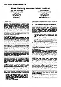
Fig. 1. Example prototype sequences from Simon and Garfunkel’s Bridge Over Troubled Water (upper left), Enya’s Once You Had Gold (upper middle), Bridge Over Troubled Water and Once You Had Gold superposed (upper right) and Once You Had Gold superposed with Mariah Carey’s Fantasy (below). The first two plots each show two different prototypes for the same song generated from different initial conditions.

3.3

Prototype Sequence Discovery

Each song is represented by a prototype sequence constructed in the following way. Input features are collected in a windowed buffer of size n (here, we let n = 120 [about 6 seconds]). When the buffer is full, the features are averaged to compute a prototype p. The buffer window is then advanced one feature and the process is repeated. Fig. 1 shows examples of prototype sequences (visualized in 2 arbitrary dimensions) for several songs, each with unique temporal structure. 3.4

Song Classification

We can now define a song timbre similarity metric: T (S 1 , S 2 ) =

P 1 X 1 ||p − p2i || P i=1 i

Algorithm 1 Classifying a Song via Prototype Sequence Similarity Require: input signal buffer s, set of prototype feature sequences {˜ pcl } 1: t = 1 2: while s buffer not empty do 3: compute feature x 4: for i = 1 to n − 1 do 5: pi = pi+1 6: pn = xP 7: p˜ = n1 pi 8: vote[t] = argminc ||˜ pct − p˜|| 9: t←t+1 10: return vote

where || · || is the L2 -norm, pci is the ith prototype in sequence fragment S c , P is the number of prototypes in the sequence fragments. Given a set of prototype sequence fragments {S i }, a new song can be classified at a particular point in time t, according to the similarity of a fragment S to those in the set: votet (S) = argmin T (S, S c ) c

Algorithm 1 gives pseudocode for this classification process. Line 3 obtains a new feature as described in Section 3.2, lines 4–6 slide and fill the prototype buffer, line 7 computes a new prototype, and line 8 compares the new prototype with the appropriate prototypes for any stored sequence fragments. Lines 1 and 9 iterate over the length of the sequence, and line 10 returns the sequence of votes for the entire song. Note that for the algorithm, the length of the song fragments compared is a single prototype point (that is P = 1). Also, note that the algorithm requires a set of prototype sequences for comparison. These might be stored in a library or accumulated in parallel from other streaming sources (for example, if the system is monitoring multiple radio stations simultaneously), but in any event, we assume that these prototype sequences are computed in a manner similar to lines 2-7 of Algorithm 1.

4

Results

We created a ten-song playlist in iTunes consisting of the songs listed in Table 1. Scottish Jig is a fast-paced bagpipe song. I Get Around is a typical Beach Boys song with a fast tempo and upbeat sound. Once You Had Gold is a mellow Enya song. I Want to Get Away is the closest thing in this playlist to hard rock and roll. Michaelangelo Sky is a standard country song with a quick beat and a bright sound. Redeemer of Israel is a choral piece with orchestral accompaniment. Fantasy is a standard Pop song with synthesized sounds and a strong beat. Time to Say Goodbye is a duet with an orchestral accompaniment. North Star is an calm acoustic guitar piece. Bridge Over Troubled Waters is primarily a piano piece with male vocals that evolves into a full instrumental accompaniment.

Table 1. Song Playlist for Training Set Number Song Name Artist 1 Scottish Jig Bagpipes 2 I Get Around Beach Boys 3 Once You Had Gold Enya 4 I Want to Get Away Lenny Kravits 5 Michaelangelo Sky Deanna Carter 6 Redeemer of Israel Mormon Tabernacle Choir 7 Fantasy Mariah Carey 8 Time to Say Goodbye Sarah Brightman and Andrea Bocelli 9 North Star Greg Simpson 10 Bridge Over Troubled Water (live) Simon and Garfunkel

We started the playlist and let the system “listen” to all ten songs as it went through the steps of the algorithm: inputting the signal, calculating and buffering the features, averaging them together to form a prototype point, and storing the sequence of prototype points. After letting the learner listen to all ten songs, we had ten prototype sequences of what had been listened to.

4.1

Auto-association Performance

Without associating a label with each prototype or song it is difficult to quantify the system’s performance. [3], [5], and [13] all use genre as the labels for songs and prototypes, but genre is not a very precise measure and does not necessarily give a good measure of similarity. [4] uses different moods as the labels for each song and prototype, but again the label is somewhat subjective. Admittedly there may not be a precise measure of similarity between songs beyond the general consensus of a song’s genre, mood, or user-defined label. And of course, for clustering imposing an additional label was not necessary. We hope to infer labels from user listening habits, such as “like” or “don’t like”. However, to first study the system behavior and as a sanity check, we tested its ability to autoassociate songs it has already stored as prototype sequences. In other words, can the system recognize music it has already heard? To make the test non-trivial and to simulate the idea of processing a novel music stream from a real-world source, we record the sound from the sound card instead of analyzing the data directly from the MP3-encoded song file. This has the effect of introducing small alignment inconsistencies as well as noise to the generated prototype sequence (which is why the two prototypes for Bridge Over Troubled Water and Once You Had Gold in Fig. 1 exhibit significant differences). Then, given a set of ten prototype sequences for the songs in the play list, we have the system “listen” again (that is, recompute a prototype sequence from the sound card output) to each song in the play list. For each song, we evaluate the distance metric for each of the stored prototypes at each point, with the minimum distance stored prototype receiving a vote at that point (line 8 of Algorithm 1).

Table 2. Auto-association Accuracy Using Prototype Sequences Number Song Name Accuracy 1 Scottish Jig 98.4% 2 I Get Around 72.4% 3 Once You Had Gold 13.1% 4 I Want to Get Away 57.1% 5 Michaelangelo Sky 41.2% 6 Redeemer of Israel 63.9% 7 Fantasy 39.8% 8 Time to Say Goodbye 58.2% 9 North Star 50.8% 10 Bridge Over Troubled Water (live) 60.1%

Table 2 reports voting accuracies that reflect the percentage of prototype points in the new song sequence that were closest to the stored sequence for that song. Results varied for each song. For some songs, the accuracy was very good, indicating that the song’s prototype was unique enough (with respect to the other stored prototypes) that alignment and noise issues did not really affect the autoassociation. For other songs, results were less impressive; given initial conditions, these songs were more easily confused with other songs’ stored prototypes. These results appear to indicate that for songs with significant temporal progression of timbre, considering this temporal information is both important and feasible even given non-ideal conditions. On the other hand, for songs with somewhat more static timbre, the temporal sequence can be misleading, as initial conditions such as noise or sequence alignment dictate more arbitrary results. 4.2

Computing Meta-Prototypes

For comparison, we now consider a compression of stored prototype sequences that eliminates temporal information (and since Algorithm 1 presents significant memory requirements this compression also relieves significant memory and processing requirements). We continue to represent the streaming source as a sequence of prototype points. For simplicity, we represent a song with a single meta-prototype point (or alternatively with a prototype sequence of length 1), essentially just averaging all prototypes in the sequence. The metaprototypes for the ten songs in the training set are given in Fig. 2, superimposed on the set of all prototype points for Bridge Over Troubled Waters. Algorithm 2 is a modified version of Algorithm 1 that compares each prototype point in the song to a single meta-prototype point for each learned song. The results of classifying the training set using this simpler scheme are shown in Table 3. Again, results varied. For a given song, the vote was often split between two or three meta-prototypes, but this seems reasonable because the music itself is not constant throughout the whole song; at times the songs truly do sound more like one song and then more like another. Let’s examine a few of the songs and see if we can understand what happened. (Recall the brief description of each

Fig. 2. Meta-prototypes for the ten songs plotted with prototypes from Bridge Over Troubled Water

song given in Section 4.) Note that, although the meta-prototypes themselves contain no temporal information, since the source is still treated in a sequential manner, the system still exhibits interesting temporal classification behavior. Let’s examine Enya’s Once You Had Gold (song number 3). Plotted in Figure 3 is the classification (which meta-prototype point was voted closest at each time t) as the song played. The x-axis is time as the song plays, and the y-axis is the index of the song that was closest to the testing example. Notice that there are no votes for the Scottish Jig, Lenny Kravits, Deanna Carter or Mariah Carey (numbers 1, 4, 5, and 7 respectively). The songs that got most of the votes were mellow songs, which makes sense. Although the prototype points did not always fall closest to the Enya meta-prototype, they did fall close to songs that shared characteristics with the Enya song. Next consider Lenny Kravit’s I Want to Get Away (song number 4), with votes plotted in Figure 4. Notice that most of the votes are distributed between

Algorithm 2 Classifying a Song via Meta-Prototype Similarity Require: input signal buffer s, set of meta-prototype features {pc } 1: t = 1 2: while s buffer not empty do 3: compute feature x 4: for i = 1 to n − 1 do 5: pi = pi+1 6: pn = xP 7: p˜ = n1 pi 8: vote[t] = argminc ||˜ pc − p˜|| 9: t←t+1 10: return vote

Table 3. Auto-association Accuracy Using Meta-Prototypes Number Song Name Accuracy 1 Scottish Jig 90.7% 2 I Get Around 100% 3 Once You Had Gold 39.7% 4 I Want to Get Away 60.1% 5 Michaelangelo Sky 36.8% 6 Redeemer of Israel 27.9% 7 Fantasy 89.4% 8 Time to Say Goodbye 13.8% 9 North Star 20.8% 10 Bridge Over Troubled Water (live) 28.4%

Lenny Kravits and Mariah Carey, the two songs that are more like Rock and Roll. This furthers our confidence in the similarity measure. Now examine Simon and Garfunkel’s Bridge Over Troubled Water (Fig. 5). Notice that there is not a clear winner, but that there seems to be clusters of votes as the song moves through time. Revisiting Fig. 1, it is obvious that this song has high variance in feature space (the figure shows just two of the twentyfour dimensions, but compared to the other songs it displayed the most variance of any of the ten songs on the playlist). For comparison, Figure 2 shows how the prototype points from Bridge Over Troubled Water relate to all the metaprototypes—it is clear that the meta-prototype for Bridge Over Troubled Water isn’t very representative of the song. 4.3

Performance on a Test Set of Novel Songs

Although we could not compute an accuracy measure in the same way, we wanted to test the same learner on songs it had not heard before. The results here seem

Fig. 3. Votes made during classification of Enya’s Once You Had Gold

Fig. 4. Votes made during classification of Lenny Kravits’s I Want to Get Away

Fig. 5. Votes made during classification of Simon and Garfunkel’s Bridge Over Troubled Water

good, but our measure is only a subjective one. We tested the learner over 30 different songs, with Figs. 6–9 showing representative voting results. With each figure we give a brief evaluation of the general classification.

5

Discussion and Future Work

We have presented an approach to measuring the similarity of streaming music content. Specifically, we give an algorithm for creating prototype sequences to model the temporal progression of a song’s timbre, and show how a minimum distance classification scheme can make use of these prototypes to auto-associate a song with itself in non-ideal streaming conditions as well as to suggest interesting (and often intuitive) similarities between different (streaming) songs. We suggest that this approach can be useful in several ways. For example, given a song that the user listens to, one might be able to predict which songs the

user would listen to in the immediate future. Such a system would be ideal for portable music players or for a system that concurrently scans multiple channels, where after only a few example songs, the system has “learned” the user’s mood. In a more static setting, given some sample ratings of songs, the system could rate an entire music library. Of course, the more examples, the better the learner would do at rating the library, especially if the collection is diverse. An obvious avenue for future work is to explore a generalization of the two algorithms that incorporates a dynamic n that can vary both within and across songs. If such a dynamic prototype size can be automatically discovered, the result should be an eclectic combination of the benefits exhibited here: compact

Fig. 6. The Verve’s Bittersweet Symphony. This song is a mix between Rock and Pop, and as might be expected it’s classified as a mix between the Rock song (number 4) and the Pop song (number 7).

Fig. 7. David Tolk’s Amazing Grace. It was classified as closest to Bridge Over Troubled Waters. Interestingly this version of Amazing Grace is mostly piano and Bridge Over Troubled Waters is the only other song that has a major piano component. Results like these were very encouraging.

Fig. 8. Sugar Ray’s When It’s Over. This Pop song was classified as closest to the Pop song we had in the training set.

Fig. 9. The Carpenter’s Rainy Days and Mondays. Interestingly it was classified as closest to the Beach Boys. This classification did not seem as logical as some of the others.

representation of global music content for each “natural” segment of a song. An intermediate step in this direction would be automating the choice of whether or not a song prototype sequence should be collapsed, based on its auto-association accuracy. Also, this automatic prototype clustering may benefit from the use of some form of (dimension specific) variance-based normalization and/or a more sophisticated compressed representation of song (meta-)prototypes, such as a mixture of Gaussians, though some of these techniques do not lend themselves naturally to the scenario of streaming sources we consider because they require processing a song in its entirety. It will also be interesting to relax the temporal alignment of songs, thus allowing the system to discover, for example, that the beginning of song A is similar to the ending of song B.

Also, at this point, our similarity metric is very simplistic—it is basically a temporal 1-NN voting scheme in the 24-dimensional space defined by the Mel cepstrum. One could substitute a more complex path similarity measure (such as Hausdorff), either again employing a periodic voting scheme (one could also experiment with more complex voting schemes), or accumulating a similarity score for each stored path over time and constantly updating the rank order of the prototypes. One could also consider higher-order path information, such as directional derivatives, as additional features. Other interesting features, from content-based information like rhythm to meta-data such as consumer purchase patterns, might also be incorporated.

References 1. Allamanche, E., Herre, J., Helmuth, O., Frba, B., Kaste, T., Cremer, M.: Contentbased identification of audio material using MPEG-7 low level description. In: Proceedings of the International Symposium of Music Information Retrieval. (2001) 2. Kim, Y., Whitman, B.: Singer identification in popular music recordings using voice coding features. In: Proceedings of the International Symposium on Music Information Retrieval. (2002) 3. Tzanetakis, G., Cook, P.: Musical genre classification of audio signals. IEEE Transactions on Speech and Audio Processing 10(5) (2002) 293–302 4. Liu, D., Lu, L., Zhang, H.J.: Automatic mood detection from acoustic music data. In: Proceedings of the International Symposium on Music Information Retrieval. (2003) 5. Pohle, T., Pampalk, E., Widmer, G.: Evaluation of frequently used audio features for classification of music into perceptual categories. In: Proceedings of the Fourth International Workshop on Content-Based Multimedia Indexing. (2005) 6. Aucouturier, J.J., Pachet, F.: Finding songs that sound the same. In: Proceedings of IEEE Benelux Workshop on Model based Processing and Coding of Audio, University of Leuven, Belgium (2002) Invited Talk. 7. Aucouturier, J.J., Pachet, F.: Scaling up music playlist generation. In: IEEE International Conference on Multimedia Expo, Lausanne (Switzerland). (2002) 8. Aucouturier, J.J., Pachet, F.: Representing musical genre: A state of art. Journal of New Music Research (JNMR) 32(1) (2003) 9. Widmer, G., Dixon, S., Knees, P., Pampalk, E., Pohle, T.: From sound to“sense” via feature extraction and machine learning: Deriving high-level descriptors for characterising music. In: Sound to Sense:Sense to Sound: A State-of-the-Art, Florence, Italy (2005) 10. Aucouturier, J.J., Pachet, F.: Music similarity measures: What’s the use? (2001) 11. Aucouturier, J.J., Sandler, M.: Segmentation of musical signals using hidden markov models. In: Proceedings of the 110th Convention of the Audio Engineering Society, Amsterdam (The Netherlands). (2001) 12. Flexer, A., Pampalk, E., Widmer, G.: Hidden markov models for spectral similarity of songs. In: Proceedings of the 8th International Conference on Digital Audio Effects (DAFx 2005), Madrid, Spain. (2005) 13. Aucouturier, J.J., Pachet, F.: Improving timbre similarity: How high is the sky? Journal of Negative Results in Speech and Audio Sciences 1(1) (2004)