âResearch supported by Research Council KUL: GOA-Mefisto 666, GOA ..... there exists a cepstral norm of a model, which we also want to express in terms of.
c 2005 International Press
COMMUNICATIONS IN INFORMATION AND SYSTEMS Vol. 5, No. 1, pp. 69-96, 2005
003
CLUSTERING TIME SERIES, SUBSPACE IDENTIFICATION AND CEPSTRAL DISTANCES∗ JEROEN BOETS† , K. DE COCK† , M. ESPINOZA† , AND B. DE MOOR†
In honor of Thomas Kailath, our friend and mentor. Ad multos annos! Abstract. In this paper a methodology to cluster time series based on measurement data is described. In particular, we propose a distance for stochastic models based on the concept of subspace angles within a model and between two models. This distance is used to obtain a clustering over the set of time series. We show how it is related to the mutual information of the past and the future output processes, and to a previously defined cepstral distance. Finally, the methodology is applied to the clustering of time series of power consumption within the Belgian electricity grid. Key words: Clustering, time series, linear models, principal angles, canonical correlations, cepstrum, mutual information
1. Introduction. Time series arise in many important areas. Some examples include the evolution of stock price indices, share prices or commodity prices, the sales figures for a particular good or service, macroeconomic and demographic indicators, image sequences, acceleration measurements by sensors on a bridge [43], ECG or EEG recordings1 , gene expression measurements at consecutive time points in bioinformatics [14], etc. Typically, the analysis is oriented to estimating a good model that can be used for monitoring, producing accurate forecasts, providing structural information and/or information about the influence of a particular set of inputs on the desired output. ∗ Research supported by Research Council KUL: GOA-Mefisto 666, GOA AMBioRICS, several PhD/postdoc & fellow grants; Flemish Government: FWO (PhD/postdoc grants, projects, G.0240.99 (multilinear algebra), G.0407.02 (support vector machines), G.0197.02 (power islands), G.0141.03 (Identification and cryptography), G.0491.03 (control for intensive care glycemia), G.0120.03 (QIT), G.0452.04 (new quantum algorithms), G.0499.04 (Robust SVM), G.0499.04 (Statistics) research communities (ICCoS, ANMMM, MLDM)); AWI (Bil. Int. Collaboration Hungary/ Poland); IWT ( PhD Grants,GBOU (McKnow)); Belgian Federal Science Policy Office: IUAP P5/22 (‘Dynamical Systems and Control: Computation, Identification and Modelling’, 2002-2006), PODO-II (CP/40: TMS and Sustainability); EU: FP5-Quprodis, ERNSI, Eureka 2063-IMPACT, Eureka 2419-FliTE; Contract Research/agreements: ISMC/IPCOS, Data4s, TML, Elia, LMS, Mastercard. † K.U.Leuven, Dept. of Electrical Engineering (ESAT-SCD), Kasteelpark Arenberg 10, B-3001 Leuven, Belgium, Tel. +32 16 32 1709, Fax +32 16 32 1970. E-mail: {jeroen.boets,katrien.decock,marcelo.espinoza,bart.demoor}@esat.kuleuven.be. Jeroen Boets is a research assistant with the Institute for the Promotion of Innovation through Science and Technology in Flanders (IWT-Vlaanderen), Belgium. Dr. Katrien De Cock is a postdoctoral researcher at the K.U.Leuven, Belgium. Marcelo Espinoza is a research assistant at the K. U. Leuven, Belgium. Prof. Dr. Bart De Moor is a full professor at the K.U.Leuven, Belgium. 1 Electrocardiogram and Electroencephalogram recordings are measurements of the electrical activity in the heart respectively the brains.
69
70
JEROEN BOETS ET AL.
However, the increasing availability of data sets consisting of a large number of time series has led to the analysis of similarities between time series. For several of the aforementioned applications it is now relevant to investigate how similar the behavior of two or more time series is, e.g. which commodities behave similarly, which sensors on a bridge are redundant, how many different types of time series exist in a given sample. These kinds of questions often arise in a broader context, where they are used as a support for strategic managerial decisions, new pricing policies, long term planning and investment decisions. One of the techniques that can be useful in providing answers is a cluster analysis [29], which is a way to find clusters of similar entities in a given data set. Distancebased clustering is built upon the definition of similarity between the objects. For the concept of similarity between time series, several suggestions have been made in the literature. Often, similarities are measured directly between the time series or a transformation of them [23]. The most straightforward choice would be to represent each time series by the vector of its measurement data and to compute e.g. the Euclidean distance or the angle between these vectors. These kinds of measures, however, have several drawbacks [45]. Longer time series can suffer from the curse of dimensionality (e.g. the ‘concentration of measure’ phenomenon as described in [13, 55]) and some of the measures are sensitive to time shifting or scaling of the measurements. Despite several adaptations such as scaling, normalization or more complex transformations of the data, these kinds of distances are not very appropriate for detecting the type of similarity we are interested in [34]. In this paper we wish to detect similarities in the dynamics of different time series, i.e. the way in which consecutive measurements are related to each other. This leads to the three-step procedure we apply in this paper for the clustering of a set of time series. This general methodology has been applied previously in different application areas such as e.g. speech processing [24] and biomedical signal processing [19]. Firstly, and this is the key step, each time series is represented by a dynamical model, which is estimated using the given data. Secondly, a distance between the dynamical models is defined and computed over all the models estimated in the first stage. Finally, a clustering and/or a classification is performed based on this distance. Each one of these steps can be filled in and implemented in its own particular way, thus giving rise to a range of different choices of design and implementation. In this paper we will mainly focus on the second step, the definition and computation of the distance. Although a lot of research has been done on defining appropriate distances for time series models [24, 18, 40, 10, 34, 4, 3], several challenges remain to be tackled. For instance, while some distances are defined and computable for both single-input single-output (SISO) and multiple-input multiple-output (MIMO) models [36, 47, 49, 7], other distances are only applicable to SISO models (e.g. the ones directly based on the cepstrum [24, 3]), opening a research challenge for the
CLUSTERING TIME SERIES, SUBSPACE IDENTIFICATION
71
multivariable extension. In this paper however, we will consider only SISO autoregressive moving average (ARMA) processes. We will define a model norm and a corresponding distance for ARMA models, based on the concept of subspace angles within and between models. We follow the approach described in [7] of defining the norm of a model by measuring the change it causes to a particular input signal, namely white noise. In contrast to the H2 norm in [7] however, we do not measure the root-mean-square gain of the output with respect to the input, but we compute the angles between the input and output spaces. This will be further explained in Section 4. A different set of questions relates to the clustering. How to graphically visualize the results of a clustering of time series when there is no explicit use of vector coordinates or they have infinite length? A possible solution for this will be described in Section 6. Practical difficulties also arise due to the fact that different clustering algorithms lead to different clustering results. Other important issues are the choice of the number of clusters, the interpretation and the evaluation of the clustering. We will come back to these issues in the application of Section 6. The paper is organized as follows (see Figure 1). In Section 2 we briefly recall the notion of principal angles between two subspaces. Section 3 describes the model class we will work with: SISO linear stochastic models. In Section 4 the subspace angles within a model and between two models are defined by applying the geometrical concept of principal angles to these models. In Section 5 we show how the (weighted) cepstral distance of [40] is related to the subspace angles between two models and how the corresponding cepstral norm relates to the angles within a model and to the mutual information of the past and future output processes. In Section 6 the distance is used for the clustering of time series of electricity demand. Section 7 concludes the paper. 2. Principal Angles between Subspaces. The concept of principal angles between two subspaces goes back to Jordan in the nineteenth century [31]. This notion was translated into the statistical notion of canonical correlations by Hotelling [26]. Applications include data analysis [20], random processes [17, 32] and stochastic realization [1, 8, 52, 54] (and references herein). Numerically stable methods to compute the principal angles and vectors via a singular value decomposition have been proposed in [5, 22] and can also be found in [21, pp. 603–604]. 2.1. Definition and Notation. The principal angles between two subspaces are a generalization of an angle between two vectors. Suppose we are given two linear subspaces S1 and S2 of the ambient space Rn of dimension d1 < n and d2 < n, respectively. A natural extension of the one-dimensional case is to choose a unit vector u1 from S1 and a unit vector v1 from S2 such that the angle between u1 and v1 is minimized. The vectors u1 and v1 so obtained, are the first principal directions
72
JEROEN BOETS ET AL.
Fig. 1. Overview of the paper.
and the angle between them is the first principal angle θ1 . Next, choose a unit vector u2 ∈ S1 orthogonal to u1 and v2 ∈ S2 orthogonal to v1 and minimize the angle θ2 between them. This is the second principal angle and u2 and v2 are the corresponding principal directions. Continue in this way until min(d1 , d2 ) angles and corresponding principal vectors have been found. This informal description is now formalized. Definition 2.1. Principal angles and directions The principal angles 0 ≤ θ1 ≤ θ2 ≤ . . . θmin(d1 ,d2 ) ≤ π/2 between the subspaces S1 and S2 of the ambient space Rn of dimension d1 < n and d2 < n, respectively, and the
CLUSTERING TIME SERIES, SUBSPACE IDENTIFICATION
73
corresponding principal directions ui ∈ S1 and vi ∈ S2 are defined recursively as cos θ1
=
cos θk
=
max uT v
= uT1 v1 ,
max uT v
= uTk vk , for k = 2, . . . , min(d1 , d2 ) ,
u∈ S1 v∈ S2
u∈ S1 v∈ S2
subject to kuk = kvk = 1 and for k > 1: uT ui = 0 and v T vi = 0, where i = 1, . . . , k−1. Let A ∈ Rp×n be of rank ra and B ∈ Rq×n of rank rb . Then, the ordered set of min(ra , rb ) principal angles between the row spaces of A and B is denoted by � θ1 , θ2 , . . . , θmin(ra ,rb ) = [A ^ B] . 2.2. The Cosines of the Principal Angles and the Principal Directions as Eigenvalues and Eigenvectors. Let A ∈ Rp×n and B ∈ Rq×n have rank ra and rb , respectively and assume that ra ≤ rb . It can be shown (see e.g. [22]) that the principal angles between and the principal directions in row(A) and row(B) follow from the symmetric generalized eigenvalue problem:
(1)
0 BAT
AB T 0
!
! x = y
AAT 0
0 BB T
!
! x λ, y
subject to xT AAT x = 1 and y T BB T y = 1. Assume that the p + q (real) eigenvalues λi are sorted in non-ascending order as λ1 ≥ . . . ≥ λp+q , then one can show that (2a)
λ1 = cos θ1 , . . . , λra = cos θra ≥ 0 ,
(2b)
λp+q = − cos θ1 , . . . , λp+q−ra +1 = − cos θra ,
(2c)
λra +1 = λra +2 = · · · = λp+q−ra = 0 .
The cosines of the ra principal angles between the row spaces of A and B are equal to the largest ra eigenvalues. The vectors AT xi and B T yi , for i = 1, . . . , ra where xi and yi satisfy (1) with λ = λi , are the principal directions corresponding to the principal angle θi . Furthermore, if A ∈ Rp×n and B ∈ Rq×n are of full row rank with p ≤ q, then the squared cosines of the principal angles between row(A) and row(B) are equal to the eigenvalues of (AAT )−1 AB T (BB T )−1 BAT : (3)
cos2 [A ^ B] = λ (AAT )−1 AB T (BB T )−1 BAT
where λ(X) denotes the eigenvalue spectrum of the matrix X.
�
,
74
JEROEN BOETS ET AL.
3. Model Class: Linear Stochastic Models. In this section, we describe the model class that we will work with, namely single-input single-output (SISO) linear time-invariant stochastic models. All models considered in this paper are assumed to be stable and minimum phase. We give the state space representation in Section 3.1. Section 3.2 recalls the observability matrix and observability Gramian. In Section 3.3 the inverse model is described and in Section 3.4 the input and output Hankel matrices are defined. 3.1. State Space Representation and Assumptions. There are many state space representations for a stochastic process {y(k)}k∈Z , all of which are equivalent, in the sense that the second order statistics of the outputs generated by the different models are the same [54, 42, 33]. We will work with the forward innovation form: ( x(k + 1) = Ax(k) + Ke(k) , (4) y(k) = Cx(k) + e(k) , where {y(k)}k∈Z ∈ R, the output of the model, is the stochastic process that is being modeled, {e(k)}k∈Z ∈ R is the innovation process of {y(k)}k∈Z and {x(k)}k∈Z ∈ Rn is the state process. The matrix A ∈ Rn×n is called the system matrix, C ∈ R1×n is the output matrix and K ∈ Rn×1 is the Kalman gain. We will denote the model (4) by the threesome (A, K, C). The transfer function from {e(k)}k∈Z to {y(k)}k∈Z is equal to H(z) = C(zIn − A)−1 K + 1 . The following assumptions are made on the input and state processes of (4). The input process {e(k)} is a zero-mean, stationary, ergodic and white stochastic process with variance σ 2 . It is assumed to be independent of the initial state. The matrix A is assumed to be stable (all of its eigenvalues lie strictly inside the unit circle) so that the state process {x(k)} is a zero-mean, stationary and ergodic stochastic process with covariance matrix Σ. Under fairly general conditions [33], the forward innovation model is minimum phase. This means that all the zeros of the model, which are the eigenvalues of A − KC, lie strictly inside the unit circle. Furthermore, the system is assumed to be minimal, so that the state covariance matrix Σ is of full rank. 3.2. The Observability Matrix and Gramian. For a specified integer i, the observability matrix Γi of the forward innovation model (4) is defined as C CA 2 (5) Γi = CA . . . . CAi−1
CLUSTERING TIME SERIES, SUBSPACE IDENTIFICATION
75
The observability Gramian Q is the solution of the observability Lyapunov equation Q = AT QA + C T C .
(6)
Since the model is stable and minimal, the matrix Q is the unique and positive definite solution of the Lyapunov equation. The explicit solution for Q is therefore given by
Q=
∞ X
(Ak )T C T CAk = ΓT∞ Γ∞ ,
k=0
where Γ∞ is the infinite observability matrix of the model. 3.3. The Inverse Model. For the stable, minimum phase and observable model (A, K, C), the inverse model is also stable and minimum phase. Its state space description is readily derived from (4): (
x(k + 1) = (A − KC)x(k) + Ky(k) , e(k) = −Cx(k) + y(k) .
We will also need the observability matrix of the inverse model, denoted by Γzi , for a specified integer i:
Γzi
−C −C(A − KC) 2 = −C(A − KC) . .. . i−1 −C(A − KC)
The observability Gramian of the inverse model is denoted by Qz and it is equal to (7)
Qz = ΓTz∞ Γz∞ .
It is the solution of the observability Lyapunov equation for the inverse model (8)
Qz = (A − KC)T Qz (A − KC) + C T C .
3.4. Input and Output Hankel Matrices. We will compute principal angles between the row spaces of input and output Hankel matrices of linear stochastic models. If s output observations y(0), y(1), . . . , y(s − 1) are given, then the output
76
JEROEN BOETS ET AL.
Hankel matrix is equal to
(9)
(10)
y(0) y(1) y(1) y(2) . .. .. . y(i − 1) y(i) Y = y(i + 1) y(i) y(i + 1) y(i + 2) .. .. . . y(2i − 1) y(2i) ! Yp = , Yf
··· ···
··· ··· ···
···
y(j − 1) y(j) .. . y(i + j − 2) , y(i + j − 1) y(i + j) .. . y(2i + j − 2)
where 2i + j − 1 = s and i and j are user-defined parameters with j � i and i larger than the model order n. The submatrix of the first i rows is denoted by Yp , where the subscript p stands for ‘past’, while the submatrix of the last i rows is Yf , the subscript f referring to the ‘future’. The past and future input Hankel matrices, Ep ∈ Ri×j and Ef ∈ Ri×j are defined in a similar way. 4. Subspace Angles between Two Models and Subspace Angles of a Model. In this section we define a notion of subspace angles between two models. They are the principal angles between certain subspaces derived from the models. The subspace angles between two models will define a distance between the models. In Section 5, we will show how these angles lead to a cepstral distance. There are also interesting angles within a model, the subspace angles of a model. They will lead to the cepstral norm of a model. We discuss the subspace angles between two models in Section 4.1 and subspace angles of a model in Section 4.2. 4.1. Subspace Angles between Two Models. 4.1.1. Definition. By looking at the principal angles between certain output spaces derived from two linear stochastic models that are driven by the same white noise sequence, we can define subspace angles between two models. Let M (1) and M (2) be SISO linear stochastic models that are driven by the same white noise sequence. The order of the models is n(1) and n(2) , respectively. The largest n(1) + n(2) principal angles between the row spaces of the output Hankel matrices can then be expressed in terms of the model parameters, while the other principal angles are all equal to 0. Theorem 4.1. The largest n(1) + n(2) principal angles between the row spaces of (1) (2) the output Hankel matrices of M (1) and M (2) , denoted � by Y �and Y� , are equal � (2) (2) (1) to the principal angles between the column spaces of Γ(1) Γz∞ and Γ∞ Γz∞ , ∞ provided the number of rows and columns of the Hankel matrices goes to ∞. The
77
CLUSTERING TIME SERIES, SUBSPACE IDENTIFICATION
other principal angles are equal to 0: h
(11)
i �� Y (1) ^ Y (2) = Γ(1) ∞
(1)
(2) Γz∞
�T � ^ Γ(2) ∞
(1) Γz∞
�T �
, 0, 0, . . . ,
(2)
(1)
(2)
where Γ∞ and Γ∞ are the observability matrices of the two models and Γz∞ and Γz∞ the observability matrices of the inverse models. The proof for the equality in (11) is given in [9, pp. 133–134]. A much more elegant proof would be possible after proving the conjecture in [11], which we offer as a challenge to the reader. � � (2) We call the principal angles between the column spaces of Γ(1) Γz∞ and ∞ � � (1) (2) Γ∞ Γz∞ the subspace angles between the two models: Definition 4.1. The subspace angles between two models The subspace angles between the model with transfer function H (1) (z) and the model (2) with transfer � as the principal angles between the column � are defined � function�H (z) (1) (2) (2) (1) spaces of Γ∞ Γz∞ and Γ∞ Γz∞ : h
H
(1)
^H
(2)
i
=
��
(1) Γ∞
(2) Γz∞
�T
^
�
(2) Γ∞
(1) Γz∞
�T �
.
It is interesting to see that the subspace angles between two models do not change when the transfer functions of the models are both multiplied by a third transfer function: Property 4.2. Consider two models with transfer function H (1) (z) and H (2) (z), respectively. A third model has transfer function H (3) (z) and is of order n(3) . Multiplying both the transfer functions H (1) and H (2) with H (3) does not change the subspace angles. It only results in 2n(3) additional subspace angles equal to 0. h
i h i H (1) H (3) ^ H (2) H (3) = H (1) ^ H (2) , 0, 0, . . . , 0 . | {z } 2n(3)
Said in other words, if two transfer functions share a common pole-zero pair, two of the subspace angles between them will be zero. 4.1.2. Computation. From the definition of the subspace angles between two models (Definition 4.1) and the expression for the cosines of the principal angles as eigenvalues in (3), it follows that the squared cosines of the subspace angles between the models with transfer function H (1) (z) and H (2) (z) are the eigenvalues of −1 Q−1 11 Q12 Q22 Q21 : (12)
h i � −1 cos2 H (1) ^ H (2) = λ Q−1 11 Q12 Q22 Q21 ,
78
JEROEN BOETS ET AL.
where
(13)
! Q11 Q12 Q= Q21 Q22 (1)T Γ∞ (2)T Γz∞ � (1) = Γ∞ (2)T Γ∞
(2)
Γz∞
(2)
Γ∞
�
(1)
Γz∞
.
(1)T
Γz∞
The matrix Q can be regarded as the observability Gramian of the model with system matrix 0 0 A(1) 0 0 0 0 (A(2) − K (2) C (2) ) , A= (2) 0 A 0 0 (1) (1) (1) 0 0 0 (A − K C ) and output matrix � C = C (1)
−C (2)
C (2)
−C (1)
�
.
Consequently, the matrix Q can be obtained by solving the Lyapunov equation: (14)
Q = AT QA + C T C .
4.2. Subspace Angles of a Model. As we will see in Section 5.2, a particular cepstral distance between two models, which was defined in [40], can be expressed in terms of the subspace angles between the models. Corresponding to the distance, there exists a cepstral norm of a model, which we also want to express in terms of principal angles. It turns out that the relevant angles are those between the input and output spaces of the model, which are discussed in Section 4.2.1. In Section 4.2.2, we look at a second group of angles, the principal angles between the past and future output spaces of a model. The two groups of angles are complementary and this complementarity will lead us to the information-theoretic interpretation of the cepstral norm in Section 5.3.2. 4.2.1. The principal Angles between Future Input and Future Output. In an analogous way as for the subspace angles between two models, we can express the principal angles between the future input and output spaces of a linear stochastic model of order n in terms of the model parameters as follows. Theorem 4.3. The largest n principal angles between the row spaces of the future input and future output Hankel matrices, Ef and Yf (see (9-10)), of a model M are equal to the principal angles between the column spaces of the observability matrix of
CLUSTERING TIME SERIES, SUBSPACE IDENTIFICATION
79
M and the observability matrix of the inverse model M −1 , provided the number of rows and columns of the Hankel matrices goes to ∞. The other principal angles are equal to 0: � � [Ef ^ Yf ] = ΓT∞ ^ ΓTz∞ , 0, 0, . . . , where Γ∞ is the observability matrix of the model and Γz∞ is the observability matrix of the inverse model. The proof of Theorem 4.3 is given in [9, p. 137]. Only n principal angles between the input and output spaces differ from 0. These angles are called the subspace angles of the model or within the model. Definition 4.2. The subspace angles of a model The subspace angles of the model M are defined as the principal angles between the column spaces of the model’s infinite observability matrix Γ∞ and the inverse model’s infinite observability matrix Γz∞ . The squared cosines of the subspace angles of the model M can be computed as the eigenvalues of Q−1 Qab Q−1 z Qba , where ! ! � Q Qab ΓT∞ � (15) = Γ Γ ∞ z ∞ Qba Qz ΓTz∞ ! ! � � A 0 is the observability Gramian of , C −C , which can be com0 A − KC puted via the observability Lyapunov equation (6). b(z) Note that the subspace angles of an nth order model M with transfer function a(z) are equal to the subspace angles between the autoregressive (AR) model with transzn zn fer function a(z) and the AR model with transfer function b(z) . They consequently indicate a certain ‘correlation’ of the pole- and zero-part of the transfer function. The closer the zeros lie to the poles, the smaller the subspace angles of the model. Conversely, the subspace angles between two models with transfer function H (1) and H (2) , H (1) respectively, are equal to the subspace angles of the model with transfer function H (2) H (2) (or H (1) ). 4.2.2. The Principal Angles between Past and Future Output. It can be shown [9, p. 121] that the principal angles between the row spaces of the past and future output Hankel matrices, Yp and Yf (see (10)), are complementary to the principal angles between the row spaces of the future input and future output Hankel matrices, Ef and Yf : (16)
[Yp ^ Yf ] =
π − [Ef ^ Yf ] . 2
We will use this complementarity in Section 5.3.2 to derive the direct relation of the cepstral norm and the mutual information of the past and future output processes.
80
JEROEN BOETS ET AL.
5. Cepstral Distance. We describe a cepstral distance and show that it can be expressed in terms of subspace angles between models (Section 5.2). Similarly, the associated cepstral norm can be expressed in terms of subspace angles within a model. This is shown in Section 5.3. In Section 5.4 we explain how the cepstral distance can be estimated from measurements. But first, we recall in Section 5.1 the definition of the cepstrum.
Fig. 2. Estimation of the cepstrum of the stochastic process {y(k)}k∈Z . The fast Fourier transform (FFT) is applied to the observations y(k) (k = 0, 1, . . . , K − 1). Next, the logarithm of the magnitude squared of the transformed sequence is normalized by the number of observations. Applying the inverse fast Fourier transform (IFFT) results in an estimate for the cepstrum.
5.1. The Cepstrum. The cepstrum of a stochastic process is defined as the inverse Fourier transform of the logarithm of the power spectrum of the process. It can be easily computed by using the fast Fourier transform, as shown in Figure 2. The cepstrum has been introduced for the detection of echoes in seismological data [6]. It is used in speech recognition [44], in fault detection methods for rotating machines [57], but also for measuring the distance between two signals, see [40, 3] and references therein. Kalpakis et al. [34] use the Euclidean distance between the cepstral coefficients of AR models to cluster time series. The cepstrum of the output process of a linear stochastic model can be expressed in terms of the model parameters. Suppose the order of the model is n, its poles are denoted by α1 , . . . , αn and the zeros by β1 , . . . , βn . Assume that the variance of the white noise input process {e(k)} is equal to σ 2 . Then, the cepstral coefficients of the output process {y(k)} are equal to [41, p. 502]: 2 k=0, log σ n n |k| (17) c(k) = X αi|k| X βi − k 6= 0 . |k| |k| i=1
i=1
The cepstrum is a real and even sequence. 5.2. A Cepstral Distance. Several distances for signals that are based on the cepstrum of the signals, have been proposed [3]. As can be seen from equation (17), the cepstral sequence of a model is in general infinitely long (although the coefficients decay to zero). That is why e.g. in the clustering approach of Kalpakis et al. [34] a finite cut-off length was chosen for the cepstral sequences, which had to be equal
CLUSTERING TIME SERIES, SUBSPACE IDENTIFICATION
81
for all time series in order to be able to compute all pairwise distances. The cepstral coefficients however do not always decay in a similar way. The closer the poles or zeros of a model are to the unit circle, the slower the decay and the more coefficients are needed. So when clustering a large set of models, the required number of coefficients to avoid false positives depends on the ‘worst’ model, i.e. the one with its poles and zeros nearest to the unit circle. The cepstral distance defined by Martin [40] does not suffer from this drawback. Due to the specific weighting of the cepstral coefficients, several closed-form formulas exist that calculate the exact distance between the (weighted) infinite cepstral sequences of the models. No explicit vector representation is needed. 5.2.1. Definition and Properties. Definition 5.1. A cepstral distance [40] Let M (1) and M (2) be two linear stochastic models with transfer function H (1) (z) and H (2) (z) and cepstrum c(1) and c(2) , respectively. Then, the squared cepstral distance between M (1) and M (2) is defined as (18)
d2 (log H (1) , log H (2) ) =
∞ X
k(c(1) (k) − c(2) (k))2 .
k=0
Note that the distance is independent of the zeroth cepstral coefficient of each process, which is equal to the logarithm of the input variance (see (17)). This implies that the distance in (18) is not a metric for ARMA processes, since a metric must obey the condition d(y (1) , y (2) ) = 0 ⇔ y (1) = y (2) . Nevertheless, it is a metric for the set of ARMA processes that are generated by sending white noise with variance 1 b(z) through an ARMA model with transfer function H(z) = a(z) , of which the polynomial coefficients b0 and a0 are equal to 1. In other words, it is a metric on that class of models. The distance belongs to a family of distances that are based on the L2 distance between the smoothed group delay spectra2 of the processes [28]. This can be shown to correspond in the cepstral domain to a certain weighting of the cepstrum. The corresponding family of weighted cepstral sequences is denoted by {w(k)c(k)} where 2 w(k) = k s exp( −k 2τ 2 ), with s and τ nonnegative parameters to be chosen. Distances are then computed as the Euclidean distances between these sequences. In our case of the cepstral distance in (18), there is no smoothing and a slight emphasis of the cepstral coefficients at higher indices k (s = 0.5), i.e. the higher quefrency components. This corresponds to stressing the more ‘quickly varying’ spectral features, resulting in sharper spectral peaks than in the unweighted case. It is easily seen that for the cepstral distance (18) the following property holds, which is similar to Property 4.2 for the subspace angles between two models. 2 The
group delay spectrum of a process with transfer function H(z) is defined as the negative derivative of the phase of the transfer function with respect to the frequency.
82
JEROEN BOETS ET AL.
Property 5.1. Let M (1) be a model with transfer function H (1) (z) and M (2) a model with transfer function H (2) (z). Consider a third model with transfer function H (3) (z). Multiplying both the transfer functions H (1) and H (2) with H (3) does not change the cepstral distance. � � �� � � � � = d log H (1) , log H (2) . d log H (1) H (3) , log H (2) H (3) This implies that in order to compute the distance between ARMA models, it is (1) (2) sufficient to consider AR models. Indeed, for H (1) (z) = ab (1)(z) and H (2) (z) = ab (2)(z) (z) (z) of order n(1) and n(2) respectively, take H (3) (z) = b(1) (z) b(2) (z) d log (1) , log (2) a (z) a (z) �
(19)
�
(1)
(2)
z n +n , b(1) (z)b(2) (z) (1)
so that
(2)
(1)
(2)
z n +n z n +n = d log (1) , log a (z)b(2) (z) a(2) (z)b(1) (z)
! .
Because M (1) and M (2) are stable and minimum phase, the two resulting AR models in (19) are stable. 5.2.2. Relation to the Subspace Angles between Two Models. As was shown in [40], by using the expression (17), the cepstral distance between two stable AR models can be expressed in terms of their poles. Let H (1) (z) and H (2) (z) be the transfer functions of stable AR models of order p and q, respectively, and with poles α1 , . . . , αp and β1 , . . . , βq . Then, the squared cepstral distance between the two models is equal to p Y q Y 1 − αi β¯j 2
(20)
� � d2 log H (1) , log H (2) = log
i=1 j=1 p Y
q Y
(1 − αi α ¯j )
i,j=1
, (1 − βi β¯j )
i,j=1
where c¯ is the complex conjugate of c. By taking a closer look at (20) for the case of two first order models, we discover an angle between two vectors. Consider the first order models with transfer function H (1) (z) and H (2) (z) and pole equal to α and β (with |α| < 1 and |β| < 1), respectively. Their squared distance equals d2 (log H (1) , log H (2) ) = log
(1 − αβ)2 1 = log , 2 2 (1 − α )(1 − β ) cos2 θ
where θ is the angle between the vectors � � � 1 α α2 · · · ∈ R∞ and 1 β
β2
···
�
∈ R∞ .
For higher order models, the squared distance as defined by Martin [40] can be expressed as the logarithm of a product of cos12 θi , where the angles θi are the subspace angles between the models:
CLUSTERING TIME SERIES, SUBSPACE IDENTIFICATION
83
Theorem 5.2. Assume the models M (1) and M (2) have transfer function H (1) (z) and H (2) (z) of order n(1) and n(2) , respectively. The cepstral distance (18) can be expressed in terms of the n(1) + n(2) subspace angles between the models M (1) and (12) (12) (12) M (2) , denoted by θ1 , θ2 , . . . , θn(1) +n(2) , as follows: (21)
2
d (log H
(1)
, log H
(2)
) = − log
n(1)Y +n(2)
(12)
cos2 θi
.
i=1
The proof of Theorem 5.2 is given in [10]. This characterization of the cepstral distance gives us a new way to compute it. Using (21) and (12), leads to −1 d2 (log H (1) , log H (2) ) = − log det Q−1 11 Q12 Q22 Q21
�
,
2
(22)
= − log
(det Q12 ) , det Q11 det Q22
where Q11 , Q12 , Q21 and Q22 are defined in (13). 5.3. A Cepstral Norm. In this section we define a cepstral norm of a model and indicate how it can be expressed in terms of the subspace angles of the model (Section 5.3.1). Its relation to the mutual information of the past and future output processes is given in Section 5.3.2. 5.3.1. Definition and Relation to the Subspace Angles in a Model. Based on the definition in [40] (see (18)), we can derive the corresponding model norm: k log Hk2 =
∞ X
kc(k)2 ,
k=0
where c(k) is the cepstrum of the model with transfer function H(z). This is equal to the Hilbert-Schmidt norm of the doubly infinite Hankel matrix of cepstral coefficients c(k), k = 1, . . . , ∞ or equivalently to the Hilbert-Schmidt-Hankel norm of log H(z) (see [12]). Note that the cepstral norm of a model is equal to the cepstral distance between the model and the model with transfer function equal to a constant (e.g. 1): k log Hk = d (log H, log 1). The cepstral norm of a model is therefore a measure for the whiteness of the output process of the model. Furthermore, the cepstral norm of an nth order b(z) model M with transfer function a(z) is equal to the cepstral distance between the zn zn autoregressive models with transfer function a(z) and b(z) , respectively. Also note that the cepstral distance between two models with transfer function H (1) and H (2) , H (1) respectively, is equal to the cepstral norm of the model with transfer function H (2)
�
H (2) H (1) H (2) (1) (2) (or H (1) ): d log H , log H = log H (2) = log H (1) . This is all similar to the observations made about the subspace angles in Section 4.2.1.
84
JEROEN BOETS ET AL.
While the cepstral distance between two models is related to the subspace angles between the models, the cepstral norm of a model is related to the subspace angles of the model. Let the model be of order n and let its subspace angles be denoted by ψ1 , ψ2 , . . . , ψn . Then, the cepstral norm is equal to ∞ X
kc(k)2 = − log
n Y
cos2 ψi .
i=1
k=0
Similarly to the cepstral distance, the norm can be computed as k log Hk2 = − log
(det Qab )2 , det Q det Qz
where Q is the observability Gramian of the model, Qz is the observability Gramian of the inverse model and Qab is equal to ΓT∞ Γz∞ (see also (15)). 5.3.2. Relation to the Mutual Information. Due to the complementarity property in (16), the norm can also be expressed in terms of the principal angles between the past and future output spaces, which are denoted by φ1 , . . . , φn : (23)
∞ X
kc(k)2 = − log
n Y
sin2 φi .
i=1
k=0
From the characterization in (23) follows that the cepstral norm of a model is proportional to the mutual information of the past and future output processes (denoted by yp and yf ), provided the output process is Gaussian. Indeed, the mutual information of the jointly Gaussian stochastic processes yp and yf can be written as (see e.g. [17]) n Y 1 sin2 φi . I(yp , yf ) = − log 2 i=1
The mutual information of the past and the future of a Gaussian stochastic output process of a linear model M with transfer function H(z) is consequently also equal to ∞
I(yp , yf ) =
1X 1 kc(k)2 = k log Hk2 . 2 2 k=0
5.4. Estimating the Cepstral Distance. Depending on the application, several ways to estimate the cepstral distance can be thought of. For instance, if one wants to cluster time series (as in the example of Section 6), one needs to estimate the cepstral distance between two time series. This is discussed in Section 5.4.1. On the other hand, in a classification problem, one has to assign a time series to one class of a set of given classes. To this end, the distance between the observation and a representative model of each class is computed and the time series is assigned to the closest class. Estimating the distance between a given model and measurements is also relevant for monitoring and fault detection. By monitoring the distance between measurements and a nominal model, one can detect changes and possibly faults in the system. How to estimate the cepstral distance between a time series and a model is explained in Section 5.4.2.
CLUSTERING TIME SERIES, SUBSPACE IDENTIFICATION
85
5.4.1. Estimating the Cepstral Distance between Two Time Series. The cepstral distance between two time series can be estimated in the following ways: 1. Assume that we use a non-parametric method for the estimation of the cepstrum (see Figure 2) of the two processes and we obtain K estimated cepstral coefficients for both, denoted by c(1) (0),. . . ,c(1) (K−1) and c(2) (0),. . . ,c(2) (K− 1). Then, the squared cepstral distance between the underlying models is approximately equal to d2 (log H (1) , log H (2) ) ≈
(24)
K−1 X
k(c(1) (k) − c(2) (k))2 .
k=1
If the cepstral coefficients were estimated exactly, the expression on the right side would be a lower bound for the exact squared distance. 2. If we identify two stochastic models, based on the two observed sequences, we can apply e.g. (22) or (20) to obtain the distance between the models. 5.4.2. Estimating the Cepstral Distance between a Time Series and a Model. Assume we have a model with transfer function H (1) (z) and K data samples y(0), . . . , y(K − 1) of a time series, originating from the model with transfer function H (2) (z). The distance between the time series and the model can be estimated in several ways. 1. By estimating the cepstrum of the time series and applying (24), where c(1) (k) (k = 1, . . . , K − 1) is the cepstrum of the model and c(2) (k) (k = 1, . . . , K − 1) is the estimated cepstrum of the time series. 2. By identifying a model based on the measurements and applying (22) or (20). 3. By applying a Kalman filter to the data. −1 Filtering the given data y(0), . . . , y(K − 1) by the inverse model H (1) (z), −1 can be seen as a series connection of the model H (2) (z) and H (1) (z). Let us denote the output of this filtering process by z(0), . . . , z(K−1). These samples thus can be viewed to originate from the ARMA model with transfer function H (2) (z) . Since the distance between H (1) and H (2) is equal to the norm H (1) (z) (2)
(z) of H , we can estimate the distance from the samples z(0), . . . , z(K − H (1) (z) 1). For example, construct the 2i × j Hankel matrix Z with the samples z(0), . . . , z(K − 1). Compute the principal angles between the row spaces of Zp and Zf and apply (23). Note that filtering the data with the inverse of the given model, can be seen as applying the Kalman filter of the model to the measurements by which the residuals of the data are determined.
6. Application: Clustering of Load Series. In this section, the methodology described is applied to a real-life clustering problem. The time series are derived from metering observations on High Voltage – Low Voltage (HV–LV) substations within the Belgian electricity grid. In Section 6.1 some background information is given. The
86
JEROEN BOETS ET AL.
data are briefly described in Section 6.2. In Section 6.3 we explain how the models are identified. Based on the models, we cluster the time series into six clusters in Section 6.4. The visualization of the clusters is explained in Section 6.5. 6.1. Background. The quantitative analysis of the electricity demand (load) is currently a key research area [46, 39] with important implications for grid managers. Not only accurate forecasts are needed for the short-term operations and mid-term scheduling, but network managers also need to have insight in the type of customers they have to supply as a support for long-term planning, pricing analysis, etc. The unbundling between generation, transmission, distribution and supply induced by the market liberalization has led to network managers being partially blind beyond a certain substation level with respect to the final customers. It is known that different types of customers (residential, industrial, business, etc.) will have a different load consumption pattern over a day; and it is also known that the load series, for any type of customer, may present important seasonal variations and weather-related effects. Therefore, usually a model has to be estimated to identify (and remove) the seasonal and weather-related effects from the load series and later on perform further analysis. The problem then is to find how many different types of time series can be identified in a sample of several time series, where each series contains the historical load measurements at a particular substation. This is, clustering of time series is required. In the literature, this problem is often tackled by using decomposition techniques to assess the types of load [37, 25]. Recently, a time series approach was proposed [15] where each hourly load series containing over 44 000 data points is represented by a 24-dimensional vector, and these vectors are clustered in a second stage. Although models were identified in [15], the distances between the time series were still measured through these representation vectors. In this paper, we compute distances between models directly, thus there is no need to build explicit representations for each time series. 6.2. Data and Model Definition. Load forecasting has been addressed by a wide range of models based on different techniques (time series analysis [2, 46, 27], neural networks applications [48, 16]) with different implementations depending on the particular objective of the model at hand. The data available for this paper consist of a set of 245 time series of hourly load values over a 5 years period (approximately 44 000 data points on each time series), where each time series is taken from an individual HV–LV substation within Belgium, provided by ELIA (Belgian National Grid Operator). Each time series, therefore, contains the historical load of a particular substation, and the goal is to perform clustering based on the similarities between substations. First, individual models are estimated for each of the 245 time series. We use the daily peak load of each time series (only measurements from working days are included) as the output of an individual model. In addition to the load
CLUSTERING TIME SERIES, SUBSPACE IDENTIFICATION
87
information, each model also includes temperature variables, to capture (and remove) the effect of weather fluctuations, and deterministic (binary) seasonal variables, to capture the load variation which is due to the cycle winter-summer within a year. 6.3. Identification of the Models. The model structure that was used for the identification of each of the 245 time series, is the linear time-invariant combined deterministic-stochastic model: ( x(k + 1) = Ax(k) + Bu(k) + Ke(k) , (25) y(k) = Cx(k) + Du(k) + e(k) , with {y(k)}k∈Z ∈ R the output of the model, {u(k)}k∈Z ∈ Rm the inputs and {e(k)}k∈Z ∈ R the innovations of the model. The variable y(k) contains the peak load value of day k, while u(k) contains three temperature variables and eleven binary seasonal variables corresponding to the months. Each model was identified using the N4SID subspace identification algorithm [53, 54], where the order of the model was chosen based on the singular values of a matrix which is obtained by obliquely projecting data matrices (see [54] for details). The data were normalized before the identification was performed. The accuracy of the models was measured by the adjusted-R2 value. This is an in-sample indicator that measures the percentage of the output variance that is explained by importing the inputs into the model, adjusted in order to penalize large numbers of inputs. One fifth of the models had an adjusted-R2 above 0.90, half of the models had one above 0.75. The worst twenty percent of the models, which had a value below 0.50, were excluded from the cluster analysis, which was done on the remaining 195 substations. 6.4. Clustering of the Substations. For the clustering of the substations only the stochastic submodel (A, K, C) of each identified full model (25) was used. In this way, all exogenous influences from the temperature and the seasons are removed and what remains are the (SISO) ARMA dynamics. To illustrate the relation of the cepstral distance and the subspace angles between two models, we consider three identified models: model 18 (order 7), model 187 (order 6) and model 190 (order 8). The distance between model 190 and model 18 is equal to 1.4106, while the distance between model 190 and model 187 is 0.2283. The subspace angles between the two pairs of models are shown in Figure 3. The cepstral coefficients (c(1), c(2), . . . , c(40)) of the three models are given in Figure 4. It is clear that the dynamics of model 187 and model 190 are very similar to each other and different from those of model 18. The cepstral distance between each pair of stochastic models was calculated through (20), resulting in a 195 × 195 distance matrix, which was used to apply an (agglomerative) hierarchical clustering algorithm. This type of algorithm initially
88
JEROEN BOETS ET AL.
70 subspace angles between model 190 and model 18 subspace angles between model 190 and model 187 60
angles in degrees
50
40
30
20
10
0
1
2
3
4
5
6
7
8
9
10
11
12
13
14
15
Fig. 3. The subspace angles between two pairs of identified models. The angles (and consequently the distance) between model 190 and model 18 are larger than the angles (and distance) between model 190 and model 187. The number of subspace angles between two models is equal to the sum of their orders. In both of the present cases the smallest angles are close to zero.
0.7 model 190 model 187 model 18 0.6
0.5
cepstrum
0.4
0.3
0.2
0.1
0
−0.1
0
5
10
15
20 k
25
30
35
40
Fig. 4. The cepstra of the three models 18 (dotted line), 187 (dash-dotted line) and 190 (full line).
CLUSTERING TIME SERIES, SUBSPACE IDENTIFICATION
89
assigns each object to a single cluster. The distance between each pair of clusters is then calculated and the pair with minimal distance is merged. This procedure is repeated until one single cluster remains. The final set of clusters is achieved by cutting the hierarchical tree at a certain level. Different types of distances between two clusters can be defined, among which e.g. the minimal, the maximal or the average distance between a member of the first and the second cluster. A different method of merging clusters is Ward’s method [56]. This method merges in each step those two clusters whose merger results in the minimal increase of information loss, which is measured by the change of the sum of squared quantization errors of representing each object by its cluster’s centroid. The method can be applied without explicit knowledge of the coordinates of the objects and was used for this application. The selection of the optimal number of clusters NC or equivalently the optimal level of cutting the hierarchical tree was achieved by maximizing over different values of NC the so-called average silhouette [35] of the resulting partition. The silhouette of an object i which belongs to a certain cluster is defined as: s(i) =
b(i) − a(i) , max(a(i), b(i))
where a(i) is the average distance from object i to the other members of its own cluster and b(i) is the minimum over all other clusters of the average distance between object i and the members of another cluster. The silhouette of an object measures how well the object belongs to its cluster and always lies between −1 (very badly) and +1 (very well). Figure 5 shows a plot of the average silhouette over the 195 substations for different choices of NC . A maximum value of 0.39 was attained for NC = 6. Figure 6 shows the matrix of all pairwise cepstral distances where the substations were rearranged according to the six clusters. To examine the influence of the clustering algorithm and the reliability of the clustering result, the procedure of clustering was also done with a different type of algorithm, namely a ‘partitioning around medoids’ (PAM) algorithm [51]. With this algorithm a maximum average silhouette of 0.38 was attained for a number of clusters NC = 5. These clusters were observed to be very close to the five clusters in Figure 6 (where the sixth cluster contains only one model). Only 12 of the 195 models (6 %) were assigned to a different cluster in both algorithms. 6.5. Visualization of the Clusters. Although Figure 6 gives a nice visualization of all distances between the models of the substations, it does not show how the models are positioned with respect to one another. In this section we will derive a way to obtain a vector representation for the models that allows such a visualization. The definition of the cepstral distance between two models (18) shows that there exists a representation for each model M (i) (i = 1, . . . , N ) that generates the given
90
JEROEN BOETS ET AL. 0.4
Average Silhouette
0.35
0.3
0.25
2
4
6
8 10 Number of Clusters NC
12
14
Fig. 5. The average silhouette for different choices of the number of clusters NC . An optimal value of 0.39 was attained for NC = 6.
distance matrix. The representation is given by the sequence {m(i) (k)}k=1,...,∞ in √ which the k th element is given by kc(i) (k), which can be calculated from the model parameters. The sequence {m(i) (k)}k=1,...,∞ is an element of the Hilbert space l2 . The Euclidean distance between two of these vectors in l2 is, by definition, equal to (18). The problem for visualization is that these vectors have infinite length, while we need two or at most three dimensions. Although for a stable and minimum phase model the sequence {m(k)}k=1,...,∞ generally decays with increasing k (see (17)), keeping only the first two or three values of the sequence would not give an optimal representation of the models with respect to the information we have about their mutual distances, especially for models with poles or zeros close to the unit circle. Therefore we propose to use another method3 , which has close links with Principal Component Analysis (PCA) [30] and kernel PCA [50]. The method starts with the following observation. Besides all pairwise distances we also know the cepstral norm of each model (computable by (20)), such that from
3 The
method we describe is equivalent to the technique of multidimensional scaling (see e.g. [38]) in the sense that the obtained visualization will be the same. In multidimensional scaling one looks for a configuration of points that realizes a given distance matrix, in this case a Euclidean. In our method the centered inner product matrix is obtained in a more obvious way.
CLUSTERING TIME SERIES, SUBSPACE IDENTIFICATION
91
Fig. 6. The matrix of all pairwise cepstral distances between the 195 substations where the stations have been rearranged according to the cluster partition with NC = 6. The color varies from black (small distances) to white (large distances). There appear to be five clusters, three of which are more dense than the others. The sixth cluster contains only one substation (on the 59th position) which clearly has a large distance to all other models. A few other outliers can also be identified, but they were assigned to one of the larger clusters.
the obvious identity for any two vectors a and b ka − bk2 = kak2 + kbk2 − 2aT b , we can immediately compute the inner product of each pair of weighted cepstral sequences of the models. This means that we know the N × N inner product matrix M T M , which in this application is a 195 × 195 matrix, and where M is the matrix with the vectors m(i) as its columns. Furthermore the matrix M T M can be transformed (i) into the inner product matrix of the centered vectors mc by the formula ! ! ~1~1T ~1~1T T T Mc Mc = IN − M M IN − , N N with ~1 ∈ RN ×1 a vector of all ones. We assume for the remainder of this section that the centering has been done.
92
JEROEN BOETS ET AL.
The following step is to project the vectors m(i) in the columns of M onto a lowerdimensional subspace while preserving as much of their variance as possible. This leads to the following solution. Let M = U SV T be the singular value decomposition (i) of M . Then, the projected vectors mpr are the columns of the matrix Mpr ∈ Rdpr ×N (with dpr < ∞), where (26)
Mpr = U T (1 : dpr , :)M = S(1 : dpr , 1 : dpr )V T (1 : dpr , :) ,
and where U T (1 : dpr , :) is the matrix with the first dpr rows of U T and all its columns and similarly for V T (1 : dpr , :). It can be proven (see e.g. [38]) that this projection is optimal in the sense that it minimizes the sum of the differences between the squared distances of the original and the projected vectors. From equation (26) it is clear that the knowledge of the inner product matrix M M suffices to obtain the matrix Mpr . Indeed, the singular values of M are the square roots of the eigenvalues of M T M and the right singular vectors of M (the columns of V ) are the eigenvectors of M T M . The percentage of variation that is retained by projecting onto the first dpr principal components can be expressed as T
Pdpr (27)
j=1
λj
j=1
λj
100 PN
,
where λj are the eigenvalues of M T M in decreasing order. Applying this to the centered inner product matrix of the 195 weighted cepstra m with dpr = 2, results in a matrix Mpr ∈ R2×195 containing the projections of m(i) onto their first two principal components. In spite of this large dimensionality reduction, 74% of the variation (as defined in (27)) was preserved. The resulting vector representation of the models is shown in Figure 7 where substations belonging to the same cluster according to the six clusters of Section 6.4 were consecutively connected by a line. (i)
7. Conclusions. In this paper we applied a general methodology for the clustering of time series, which basically consists of the following three steps. • Associate a dynamical model with each time series. • Choose or define a distance for these models. • Perform a cluster analysis based on the chosen distance. We proposed for this procedure a particular distance for SISO linear stochastic models (ARMA models), based on the concept of subspace angles within a model and between two models. These angles are defined as the principal angles between certain subspaces derived from the models. The distance we proposed, which is a particular combination of these angles, was shown to be equal to a previously defined distance based on the cepstrum of the models. The corresponding model norm was proven to be related to the mutual information of the past and the future output processes of the model.
93
CLUSTERING TIME SERIES, SUBSPACE IDENTIFICATION M
pr
1.2
1
0.8
Principal Component 2
0.6
0.4
0.2
0
−0.2
−0.4
−0.6 −1.5
−1
−0.5 0 Principal Component 1
0.5
1
Fig. 7. The resulting two-dimensional vector representation of the models. Each cross on the figure corresponds to the model of a substation. Substations belonging to the same cluster according to the cluster partition obtained in Section 6.4 are consecutively connected by a line. The ordering is the same as in Figure 6. Clearly the five clusters can still be recognized with 74 percent of the information preserved. The object of the sixth cluster has lost its distinctive position.
We applied this methodology to a set of time series of power demand from the Belgian electricity grid. In the first step, models were obtained through subspace identification. The chosen distance was the (weighted) cepstral distance described in this paper. In the third step, a cluster analysis was performed with a hierarchical clustering algorithm and an optimal partitioning obtained by selecting the one with the highest average silhouette. Five clusters appeared to be present, while the sixth contained only an outlier model. Finally, we described a method to visualize the models in a two-dimensional plane. Our further research will be on the investigation of differences between the proposed cepstral distance and other existing distances (see e.g. the references in Section 1), as well as on the extension of the distance to MIMO models. As far as we know, a definition of the cepstrum for multivariable models does not exist. The concept of subspace angles within and between MIMO models can give some ideas to establish this. Another interesting issue is the computational complexity of our approach in the case where a large set of time series is given. Based on the various ways of calculating the cepstral distance described in Section 5.4, different clustering approaches can be thought of. We wish to investigate the possibility and (dis)advantages
94
JEROEN BOETS ET AL.
of not estimating all models beforehand, but making use of the formulas in Section 5.4 and using a mixed procedure of clustering and classification.
REFERENCES [1] H. Akaike, Stochastic theory of minimal realization, IEEE Transactions on Automatic Control, 19(1974), pp. 667–674. [2] N. Amjady, Short-term hourly load forecasting using time-series modeling with peak load estimation capability, IEEE Transactions on Power Systems, 16:4(2001), pp. 798–805. [3] M. Basseville, Distance measures for signal processing and pattern recognition, Signal Processing, 18:4(1989), pp. 349–369. [4] A. Bissacco, A. Chiuso, Y. Ma, and S. Soatto, Recognition of human gaits, in: Proceedings of the IEEE International Conference on Computer Vision and Pattern Recognition (CVPR 01), volume 2, pages 52–58, Kauai, Hawaii, December 2001. Also available as black1.csl.uiuc.edu/˜yima/psfile/gait rcgntn.ps.gz. ¨ rck and G. H. Golub, Numerical methods for computing angles between linear sub[5] ˚ A. Bjo spaces, Mathematics of Computation, 27(1973), pp. 579–594. [6] B. P. Bogert, M. J. R. Healy, and J. W. Tukey, The quefrency alanysis of time series for echoes: cepstrum, pseudo-autocovariance, cross-cepstrum and saphe cracking, in: M. Rosenblat, editor, Proceedings of the Symposium on Time Series Analysis, pages 209– 243. Wiley, New York, 1963. [7] S. P. Boyd and C. H. Barratt, Linear Controller Design: Limits of Performance, Prentice Hall, Englewood Cliffs, New Jersey, 1991. [8] P. E. Caines, Linear Stochastic Systems, Wiley, New York, 1988. [9] K. De Cock, Principal Angles in System Theory, Information theory and Signal Processing, PhD thesis, K.U.Leuven, Faculty of Applied Sciences, Leuven, Belgium, 2002. Available as ftp://ftp.esat.kuleuven.ac.be/pub/SISTA/decock/reports/phd.ps.gz. [10] K. De Cock and B. De Moor, Subspace angles between ARMA models, Systems & Control Letters, 46:4(2002), pp. 265–270. [11] K. De Cock and B. De Moor, A conjecture on Lyapunov equations and principal angles in subspace identification, in: V. D. Blondel and A. Megretski, editors, Unsolved Problems in Mathematical Systems and Control Theory, pages 287–292. Princeton University Press, 2004. Available on http://pup.princeton.edu/math/blondel/. [12] K. De Cock, B. Hanzon, and B. De Moor, On a cepstral norm for an ARMA model and the polar plot of the logarithm of its transfer function, Signal Processing, 83:2(2003), pp. 439–443. [13] P. Demartines, Analyse de Donn´ ees par R´ eseaux de Neurones Auto-organis´ es (Data Analysis through Self-organized Neural Networks), PhD thesis, Institut National Polytechnique de Grenoble, Grenoble, France, 1994. [14] D. J. Duggan, M. Bittner, Y. Chen, P. Meltzer, and J. M. Trent, Expression profiling using cDNA microarrays, Nature Genetics, 21(1999), pp. 10–14. [15] M. Espinoza, C. Joye, R. Belmans, and B. De Moor, Short-term load forecasting, profile identification and customer segmentation: A methodology based on periodic time series, IEEE Transactions on Power Systems, 20:3(2005), pp. 1622–1630. [16] D. Fay, J. Ringwood, M. Condon, and M. Kelly, 24-h electrical load data–a sequential or partitioned time series? Neurocomputing, 55:3(2003), pp. 469–498. [17] I. M. Gel’fand and A. M. Yaglom, Calculation of the amount of information about a random function contained in another such function, American Mathematical Society Translations, Series (2), 12(1959), pp. 199–236.
CLUSTERING TIME SERIES, SUBSPACE IDENTIFICATION
95
[18] T. T. Georgiou and A. Lindquist, Kullback-Leibler approximation of spectral density functions, IEEE Transactions on Information Theory, 49:11(2003), pp. 2910–2917. [19] W. Gersch, Nearest neighbor rule in classification of stationary and nonstationary time series, in: D. F. Findley, editor, Applied Time Series Analysis II, pages 221–270. Academic Press, New York, 1981. [20] R. Gittins, Canonical Analysis: a Review with Applications in Ecology, Springer, Berlin, 1985. [21] G. H. Golub and C. F. Van Loan, Matrix Computations, The Johns Hopkins University Press, Baltimore, 1996. [22] G. H. Golub and H. Zha, The canonical correlations of matrix pairs and their numerical computation, in: A. Bojanczyk and G. Cybenko, editors, Linear Algebra for Signal Processing, pages 59–82. Springer, New York, 1995. [23] A. Gordon, Classification, Chapman-Hall, 1999. [24] R. M. Gray, A. Buzo, A. H. Gray, Jr., and Y. Matsuyama, Distortion measures for speech processing, IEEE Transactions on Acoustics, Speech, and Signal Processing, 28:4(1980), pp. 367–376. [25] S. Heunis and R. Herman, A probabilistic model for residential consumer loads, IEEE Transactions on Power Systems, 17:3(2002), pp. 621–625. [26] H. Hotelling, Relations between two sets of variates, Biometrika, 28(1936), pp. 321–372. [27] S-J. Huang and K-R. Shih, Short term load forecasting via ARMA model identification including non-Gaussian process considerations, IEEE Transactions on Power Systems, 18:2(2003), pp. 673–679. [28] F. Itakura and T. Umezaki, Distance measure for speech recognition based on the smoothed group delay spectrum, in: Proceedings of the IEEE International Conference on Acoustics, Speech and Signal Processing (ICASSP87), volume 3, pages 1257–1260, 1987. [29] A. K. Jain and R. C. Dubes, Algorithms for Clustering Data, Prentice Hall, Englewood Cliffs, NJ, 1988. [30] I. T. Jolliffe, Principal Component Analysis, Springer-Verlag, New York, Berlin, Heidelberg, Tokyo, 1990. [31] C. Jordan, Essai sur la g´ eom´ etrie ` a n dimensions, Bulletin de la Soci´ et´ e Math´ ematique, 3(1875), pp. 103–174. [32] T. Kailath, A view of three decades of linear filtering theory, IEEE Transactions on Information Theory, 20(1974), pp. 146–181. [33] T. Kailath, A. H. Sayed, and B. Hassibi, Linear Estimation, Prentice Hall, Upper Saddle River, NJ, 2000. [34] K. Kalpakis, D. Gada, and V. Puttagunta, Distance measures for effective clustering of ARIMA time-series, in: Proceedings of the 2001 IEEE International Conference on Data Mining (ICDM’01), pages 273–280, San Jose, CA, November-December 2001. Available as http://www.csee.umbc.edu/˜kalpakis/homepage/papers/ICDM01.pdf. [35] L. Kaufman and P. Rousseeuw, Finding Groups in Data: An Introduction to Cluster Analysis, John Wiley & Sons, New York, 1990. [36] D. Kazakos and P. Papantoni-Kazakos, Detection and Estimation, Computer Science Press, 1990. [37] H. Liao and D. Niebur, Load profile estimation in electric transmission networks using independent component analysis, IEEE Transactions on Power Systems, 18:2(2003), pp. 707–715. [38] K. V. Mardia, J. T. Kent, and J. M. Bibby, Multivariate Analysis, Academic Press, London, New York, Toronto, Sydney, San Francisco, 1979. [39] E. Mariani and S. S. Murthy, Advanced Load Dispatch for Power Systems, Advances in Industrial Control, Springer-Verlag, 1997.
96
JEROEN BOETS ET AL.
[40] R. J. Martin, A metric for ARMA processes, IEEE Transactions on Signal Processing 48:4(2000), pp. 1164–1170. [41] A. V. Oppenheim and R. W. Schafer, Digital Signal Processing, Prentice Hall International, London, 1975. [42] D. Pal, Balanced stochastic realization and model reduction, Master’s thesis, Washington State University, Electrical Engineering, 1982. [43] B. Peeters, System Identification and Damage Detection in Civil Engineering, PhD thesis, Faculty of Engineering, K.U.Leuven, Leuven (Belgium), 2000. Available as http://www.kuleuven.ac.be/bwm/papersBartPeeters PhD.pdf. [44] L. R. Rabiner and B. H. Juang, Fundamentals of Speech Recognition, Prentice Hall, Englewood Cliffs, NJ, 1993. [45] D. Rafiei, On similarity-based queries for time series data, in: Proceedings of International Conference on Data Engineering, pages 410–417, Sydney, Australia, March 1999. [46] R. Ramanathan, R. F. Engle, C. W. J. Granger, F. Vahid-Araghi, and C. Brace, Shortrun forecasts of electricity loads and peaks, International Journal of Forecasting, 13:2(1997), pp. 161–174. [47] F. C. Schweppe, On the Bhattacharyya distance and the divergence between Gaussian processes, Information and Control, 11:4(1967), pp. 373–395. [48] H. Steinherz, C. Pedreira, and R. Castro, Neural networks for short-term load forecasting: A review and evaluation, IEEE Transactions on Power Systems, 16:1(2001). [49] A. A. Stoorvogel and J. H. van Schuppen, System identification with information theoretic criteria, in: S. Bittanti and G. Picci, editors, Identification, Adaptation, Learning, pages 289–338. Springer, Berlin, 1996. Also available on http://www.cwi.nl/ftp/CWIreports/BS/ as file BS-R9513.ps.Z. [50] J. A. K. Suykens, T. Van Gestel, J. De Brabanter, B. De Moor, and J. Vandewalle, Least Squares Support Vector Machines, World Scientific, Singapore, 2002. [51] M. J. van der Laan, K. S. Pollard, and J. Bryan, A new partitioning around medoids algorithm, Journal of Statistical Computation and Simulation, 73:8(2003), pp. 575–584. [52] P. Van Overschee and B. De Moor, Subspace algorithms for the stochastic identification problem, Automatica, 29(1993), pp. 649–660. [53] P. Van Overschee and B. De Moor, N4SID – Subspace algorithms for the identification of combined deterministic-stochastic systems, Automatica, 30:1(1994), pp. 75–94. [54] P. Van Overschee and B. De Moor, Subspace Identification for Linear Systems: Theory – Implementation – Applications, Kluwer Academic Publishers, Boston, 1996. Also available as ftp://ftp.esat.kuleuven.ac.be/pub/SISTA/nackaerts/other/alln.ps.gz. [55] M. Verleysen, D. Franc ¸ ois, G. Simon, and V. Wertz, On the effects of dimensionality on data analysis with neural networks, in: IWANN 2003, International Work-Conference on Artificial and Natural Neural Networks, pages 209–243, Mao, Menorca (Spain), June 3–6, 2003. [56] J. H. Ward, Hierarchical grouping to optimize an objective function, Journal of the American Statistical Association, 58(1963), pp. 236–244. [57] J. Wismer, Application Note: Gearbox Analysis Using Cepstrum Analysis and Comb Liftering, Br¨ uel & Kjær, Denmark.