This paper was prepared for presentation at the Carbon Management Technology Conference held in Sugarland, Texas, USA, 17â19 November 2015.
CMTC-439489-MS Quantifying Local Capillary Trapping Storage Capacity Using Geologic Criteria Bo Ren, The University of Texas at Austin, Steven L. Bryant, University of Calgary and Larry W. Lake, The University of Texas at Austin
Copyright 2015, Carbon Management Technology Conference This paper was prepared for presentation at the Carbon Management Technology Conference held in Sugarland, Texas, USA, 17 –19 November 2015. This paper was selected for presentation by a CMTC program committee following review of information contained in an abstract submitted by the author(s). Contents of the paper have not been reviewed and are subject to correction by the author(s). The material does not necessarily reflect any position of the Carbon Management Technology Conference, its officers, or members. Electronic reproduction, distribution, or storage of any part of this paper without the written consent of the Carbon Management Technology Conference is prohibited. Permission to reproduce in print is restricted to an abstract of not more than 300 words; illustrations may not be copied. The abstract must contain conspicuous acknowledgment of CMTC copyright.
Abstract The capillary pressure heterogeneity or local capillary trapping (LCT) determines the final distribution of CO2 in a saline aquifer during geological carbon sequestration. This locally trapped CO2 would not escape from the storage formation even if caprock integrity is compromised. It is, therefore, essential to predict the extent and storage capacity of LCT during the design of GCS projects. This work employs a fast method based on the geologic criteria to estimate the structures of local capillary traps. The method assumes a critical capillary entry pressure (CCEP) and a geostatistical realization of the reservoir entry pressure field as inputs. It then finds the capillary barriers inside the domain and identifies the grid blocks beneath clusters of barriers. These grid blocks are the local capillary traps. The criterion for choosing the CCEP is important, and we suggest a criterion in this work. We verify this algorithm by full-physics simulations in small 2D and 3D domains. We employ a large CO2 injection rate (Ngr~0.1) to fully sweep the storage domain, followed by a long period of buoyant flow to allow for complete charging of those local capillary traps. We test several CCEPs to determine the most physically representative value by comparing the LCT predicted from both methods. We find that a single value of CCEP enables the geologic algorithm to give a very good approximation of LCT distribution as well as LCT volume in uncorrelated and weakly correlated porous media. This means that the concept of CCEP is a reasonable approximation to the physical process by which traps are filled. LCT can be described in terms of percolation theory. The percolation threshold arises from the competition between connected clusters of barriers and connected clusters of local traps. We show that both the percolated CCEP (corresponding to the percolation of LCT) and optimal CCEP (corresponding to the best match between geologic criteria and full-physics simulation) change with each other in a predictable linear way for the uncorrelated capillary entry pressure field.
CMTC-439489-MS
2
Introduction Geological CO2 sequestration (GCS) in the saline aquifer has been widely accepted as the most promising and easily accessible way to reduce the carbon emissions and global warming (Bachu, 2008). One of the main concerns is whether the CO2 can be permanently stored in a safe way. In order to achieve this, it is essential to understand the CO2 migration behavior, storage state and leakage characteristics. After CO2 injection, four widely accepted storage mechanism are responsible for immobilizing CO2 in the storage formation. They are structural, solubility, residual, and mineral trapping. Quantitatively, the relative importance of these different trapping mechanisms over time depends on several factors, such as geometry of formations, permeability and its distribution, injection rate, and wettability (Doughty, 2007; Juanes et al., 2006; Kumar et al., 2005; Mo and Akervoll, 2005, Saadatpoor, 2009, Taku Ide et al., 2007). Recently, a new trapping mechanism called local capillary trapping was proposed in reservoirs exhibiting capillary pressure heterogeneity (Saadatpoor et al., 2009). Specifically, it occurs during buoyancy-driven migration of bulk phase CO2 within a saline aquifer with spatially varying petrophysical properties (permeability and capillary entry pressure). The most important benefit of LCT is that saturation of the stored CO2 in the LCT is larger than that predicted for other trapping mechanisms, and CO2 in these regions of locally large saturation will not escape from the formation even if caprock integrity or other geomechanical disruptions occur in the long-term sequestration period. Ren (Ren et al., 2014) demonstrated that the LCT can be as significant as residual trapping in immobilizing CO2 into the storage domain. Taking no account of the LCT would consequently overestimate the CO2 leakage flux, amount, and risks. Additionally, these local accumulations of CO2 patches would significantly impact the seismic response and imaging during the monitoring period (Behzadi et al., 2011, Meckel et al., 2015). Therefore, it is essential to predict and quantify the amount, extent and distribution of LCT during GCS in the saline aquifer. A number of simulation studies have been conducted to investigate the impact of capillary heterogeneity (Behzadi and Alvarado, 2012; Kong et al., 2014; Li and Benson, 2015; Mouche et al., 2010; Saadatpoor, 2012) on the CO2 upward migration, saturation distribution, and trapping state. The main issue of these simulations is the long run time because of the incorporation of this small-scale capillary heterogeneity. Considering this, Saadatpoor (Saadatpoor, 2012) developed a fast algorithm to predict the LCT distribution and capacity based on the geologic model, specifically on the entry capillary pressure field which is correlated with permeability field. A critical capillary entry pressure (CCEP) is assumed that will determine the grid blocks to be barriers or flow path and then find the flow path grids surrounded by barriers. These flow path grid blocks are the LCT. The algorithm is tested by simulations of buoyant flow and it is found the algorithm always predicts some “false” LCTs not observed in the full-physics simulation because CO2 does not sweep these grids during buoyancy-driven flow. The other issue with the algorithm is the identification of the CCEP a priori. The objective of this work is to test the applicability of the geologic algorithm when the CO2 is emplaced in the reservoir by injection and how to determine the value of CCEP. During the injection period of CO2, viscous forces can enable the CO2 to invade much of the pore space near the wellbore regardless of capillary heterogeneity. Thus the initial state of the buoyancy-dominated flow period differs significantly from some previous studies, and the occupancy and saturation of LCTs attained during post-injection buoyancy driven flow could therefore differ as well.
Description of Geologic Criteria Algorithm The following subroutines can be applied to both 2D and 3D capillary entry pressure fields. 1. Given a value of critical capillary entry pressure, find all cells in the domain that have entry pressure exceeding the critical value of CCEP (=2 psi). Fig. 1a shows a sample 2D capillary entry
CMTC-439489-MS
3
pressure field and Fig. 1b shows barrier grid blocks in the orange that have capillary entry pressure larger than CCEP.
(a) (b) Fig. 1. (a) Heterogeneous capillary entry pressure (2D sample); (b) Orange cells have capillary entry pressure larger than CCEP and are considered as barriers. 2. All the connected clusters of barriers in the set of cells from step 1.
Fig. 2. The connected cluster of barriers shown in the red blocks. 3. Find the non-barrier clusters that are surrounded by the set of clusters of barriers from step 2.
Fig. 3. The local capillary traps are shown in the green blocks.
2D/3D Geologic Model Construction We built 2D and 3D statistical geologic models. The model dimensions and properties are shown in Table 1. The porosity field is correlated with permeability by the Eq. 1 (Holtz, 2002). The capillary entry pressure field is generated by the Leverett J-function (Leverett, 1941) which correlates the permeability, porosity, and entry capillary pressure together. The Leverett J-function is shown in Eq. 2.
7E 7 k
J (Sw )
1 / 9 .6 1
pc (S w )
g /w
cos
…………………………………………..(1) k
………………………………………. (2)
In the above equation, 𝑝𝑐 is the capillary pressure, 𝜎 is the interfacial tension between CO2 and brine, 𝜃 is the contact angle, 𝑘 is the permeability, 𝜙 is the porosity. To scale the capillary pressure curve for each grid block in the aquifer, we assume that the interfacial tension and contact angle do not vary spatially. We also assume that the shape of capillary pressure curve does not vary spatially. Thus for arbitrary grid block 𝑖 and 𝑗, we can transform Eq. 2 into Eq. 3.
CMTC-439489-MS
4
p ci ( S w ) p cj ( S w )
kj ki
*
i j
………………………………………(3)
Subscript 𝑗 denotes the properties of the rock for which we know the capillary pressure curve, and we call it reference rock. 𝜙𝑗 and 𝑘𝑗 are the reference permeability and porosity, respectively. We assign the reference capillary pressure curve to the grids block with the average permeability, and capillary pressure curves for other grids can be calculated by Eq. 3. The generated 2D capillary entry pressure field and its histogram are shown in Fig. 4a and 4b, respectively. The corresponding 3D fields are shown in Fig. 5a and 5b. Table 1. 2D and 3D Geologic Model Parameters Model parameters 2D Model dimension (𝑁𝑥, 𝑁𝑦, 𝑁𝑧 ), ft 400 × 100 Grid block size, ft 1×1 Permeability field lognormal Auto correlation length (𝐿𝑥, 𝐿𝑦, 𝐿𝑧), ft (5,~, 0) Mean of permeability, mD 194 Anisotropy of permeability field, isotropic Standard deviation of permeability, mD 339 Porosity, constant 0.269 2.07 Mean of capillary entry pressure (µ), psi 1.36 Standard deviation of capillary entry pressure (𝜎), psi
(a) 2D capillary entry pressure field (psi)
(b) Capillary entry pressure histogram in 2D Fig. 4. 2D capillary entry pressure and histogram
3D 64 × 32 × 32 1×1×1 lognormal (5, 5, 0) 403 isotropic 774 0.269 2.13 1.43
(a) 3D capillary entry pressure field (psi)
(b) Capillary entry pressure histogram in 3D Fig. 5. 3D capillary entry pressure and histogram
Simulation Settings in the CMG-GEM We employ the simulator of CMG-GEM (CMG, 2012) to conduct the CO2 flow simulation in the above 2D and 3D geologic models. The fluid properties of CO2 and brine are the same as before (Kumar, 2005). The relative permeability curve and reference capillary pressure curve are shown Fig. 6 and Fig.7, respectively. Hysteresis in the relative permeability is considered but not in capillary pressure.
CMTC-439489-MS
5
The capillary pressure curve for each grid was scaled by the Leverett J-function and the reference capillary pressure curve as described above.
Fig. 6. Relative permeability curves
Fig. 7. Reference capillary pressure curve
The simulation injection scheme is shown in Table 2. In the CMG-GEM, we employ a very large VOLMOD in the right boundary grid blocks to mimic the open flow boundary. We select the injected volume to be enough to fill the storage domain, but it accounts for little (4.2E-5) of the total pore volume. The injection period is short considering the small storage domain, and after injection, we continue to run the simulation to allow for the buoyant flow, during which LCT would be filled, to reach a steady state. The period during injection and post-injection lasts for 50 years. The Darcy velocity along the wellbore for 2D is set to be same as that of 3D. The buoyancy number along the wellbore perforation for 2D and 3D is calculated based on the following equation and shown in Table 2. N
gr
gkvL u H
……………………………………………(4)
In In the above equation, 𝑁𝑔𝑟 is the buoyancy number, ∆𝜌 is density difference between brine and CO2 (405.9 kg/m3), 𝑔 is buoyancy constant, 𝑘𝑣 is the average vertical permeability (see Table 1), 𝑢 is the Darcy velocity of CO2 along the wellbore, 𝑢 = 𝑞/(2𝜋𝑟𝑤 𝐻), 𝑞 is the injection rate, 𝑟𝑤 is the wellbore radius. 𝜇 is the viscosity of CO2 (0.049 mPa•s), 𝐿 is the reservoir length, 𝐻 is the perforated length. Table 2. Injection simulation scheme in the CMG-GEM Parameters 2D 3D Well type Vertical Vertical Perforation interval Left lower quarter Left middle lower half Perforation length, ft 25 16 Injection rate, Scf/d 4.9E+5 3.1E+5 Injection period, day 73 70 Simulation period, yr 50 50 Buoyancy number along wellbore 0.1 0.2
Results from Geologic Criteria Algorithm Since the local capillary trap is surrounded by the grid blocks with the locally larger capillary entry pressure, we expect that the best CCEP will be very close to the mean of the capillary entry pressure field. Based on the histogram of capillary entry pressure as shown in the Fig. 4b and Fig. 5b, we select several values of CCEP around the mean of capillary entry pressure. They are from 0.80 through 2.0 psi
CMTC-439489-MS
6
with the interval of 0.05 psi. Fig. 8a shows the variation of LCT volume fraction under different values of CCEP in the 3D. Here, the LCT volume fraction is defined as the number of LCT grid blocks divided by the total number of grid blocks of the storage domain. The CCEP is normalized by the mean and standard deviation of the capillary entry pressure. We can see from Fig. 8a that LCT volume fraction first increases with the CCEP followed by a decrease. The increasing part of the trend is simply because as the CCEP increases, more grid blocks become flow paths instead of barriers, and since most of the domain is a barrier at small CCEP, the additional flow paths are also additional LCT. However, increasing CCEP also decreases the number of barrier grid blocks, which is necessary to surround the LCT grids, and eventually the number of possible LCT must decrease. Therefore, there exists a threshold value of CCEP which gives rise to the maximum LCT volume fraction. In this example, the threshold CCEP is 1.05 psi and the corresponding LCT volume fraction is 16%. Fig. 8b shows the LCT distribution and different sizes of LCT clusters under the threshold CCEP of 1.05 psi. Total 753 clusters of LCT is detected and the largest LCT cluster (ID=2) has 3731 grid blocks (5.69% of the whole domain). In the future publication, we will show the LCT cluster size distribution and fractal behavior analysis in detail. We label the LCT cluster ID from the bottom middle grid block, and it can be observed that even for the largest LCT cluster (ID=2), it cannot span the whole domain from the bottom to the top. This phenomenon is different from the traditional invasion percolation theory (Wilkinson and Willemsen, 1983). However, to be simple, we still call the CCEP at which gives the largest LCT fraction as the ‘percolated CCEP’. In the following section of comparison of LCT between geologic criteria and CMG-GEM, we will show LCT for a range of closely spaced CCEP values and try to identify the optimal CCEP that could give the best match with the CMG-GEM.
(a) (b) Fig. 8. (a) LCT volume fraction versus CCEP in the 3D, µ=2.13 psi, 𝜎=1.43 psi (refer to Table 1); (b) LCT clusters in the domain under the percolated CCEP 1.05 psi; colors are arbitrary.
Results from CMG-GEM The CO2 saturation at the end of the injection in 2D storage domain is shown in Fig. 9a. It can be seen that CO2 is in the compact displacement under the high injection rate and CO2 displaces brine almost everywhere, though not to the same saturation. Clearly all the local capillary traps that are intrinsic to the geologic model are occupied by CO2 at the end of injection. We then continued the simulation to allow buoyant flow. The CO2 saturation at the end of buoyant flow is shown in the Fig. 9b, the yellow and red color grid blocks with high CO2 saturation are the LCT. Fig. 9c and 9d show the histogram of the CO2 saturation at the end of both injection and buoyant flow, respectively. The CO2 saturation at the end of injection mostly follows the normal distribution with the mean value of 0.63. This is consistent with others’ observation from coreflooding experiments (Kong et al., 2014; Krause, 2012). However, after buoyant flow, two peaks of saturation frequency are observed, one is around the residual gas saturation (0.287), and the other peak is around 0.8 (1-Swirr), which is the local capillary trapping. The corresponding results for the 3D are shown in Fig. 10. It should be noted that LCT frequency (CO2 saturation larger than 0.75 is assumed as LCT) in 3D is half of that for 2D.
CMTC-439489-MS
7
(a). CO2 saturation at the end of injection
(b). CO2 saturation at the end of buoyant flow
(c). CO2 saturation histogram of (a) (d). CO2 saturation histogram of (b) Fig. 9. CO2 saturation distribution and histogram in 2D model.
(d). CO2 saturation histogram of (a) Fig. 10. CO2 saturation distribution and histogram in the 3D model.
(a). CO2 saturation distribution at the end of buoyant flow
Comparison of LCT between Geologic Criteria and CMG-GEM After we obtain the LCT saturation distribution from CMG-GEM, we extract the LCT from the saturations map at the end of buoyant flow (see Fig. 9b and Fig. 10a) and compare them with the LCT from the geologic algorithm. Grid block with CO2 saturation higher than 0.75 is assumed as LCT. We define a match index (Eq. 5) to search for the optimal CCEP. It is defined as the ratio of the grids predicted from both methods over the sum of the number of grids predicted only from CMG-GEM and that predicted only from geologic criteria. Therefore, the match index ranges from 0 to 1. The worst match has the match index that approaches to 0 while the best match approaches to 1. The CCEP corresponding to the peaked match index would be the optimal CCEP. The changes of LCT volume fraction and match index with CCEP in the 2D simulation are shown in left plot of Fig. 11. It can be observed the CCEP corresponding to the peak value of LCT volume fraction is equal to 1.8 psi, while the optimal CCEP that gives the best match is 1.15 psi. We also show the comparison under the optimal CCEP in the left plot of Fig. 12. In the figure, if a grid block is predicted as LCT from both methods, we set it to be green. If the grid block is predicted as LCT only from CME-GEM and geologic criteria, we set them to be red and blue, respectively. The LCT volume fraction predicted from the geologic criteria under the optimal CCEP is 25% while it is 20% as predicted from CMG-GEM. Similarly, we conduct a 3D analysis on the optimal CCEP and the result is shown in the right plot of
CMTC-439489-MS
8
Fig. 11. The optimal CCEP is found to be the same as the percolated CCEP. The corresponding comparison of LCT between the two methods in several selected layers of the reservoir is shown in Fig. 12. It can be observed that LCT from the geologic criteria could fully and exactly represent the LCT from the CMG-GEM under the optimal CCEP. However, geologic criteria overestimates LCT as we have some “false” blue grid blocks only predicted from the geologic criteria. The LCT volume fraction from the geologic criteria under the optimal CCEP is 16% while it is 7% as predicted from CMG-GEM. M. I = LCT from both methods (# green grid) …....(5) (# (# LCT from both methods
green grid)+LCT from CMG−GEM only
red grid)+LCT only from GC only (# blue grid)
Fig. 11. LCT volume fraction and match index (Eq. 5) vary with CCEP in 2D (left) and 3D (right).
Fig. 12. Comparison of LCT between CMG-GEM and geologic criteria algorithm under the optimal CCEP. Left: 2D with the optimal CCEP=1.15 psi. For the comparison, we exclude the top 11 layer with high saturation CO2 accumulation beneath the seal and the right 50 columns with CO2 dissolved in brine (refer to Fig. 9b). Right: 3D in layer 2 through 7 from top to the bottom of the domain under the optimal CCEP =1.05 psi. We exclude the top four layers with high saturation CO2 accumulation beneath the seal and the right fourteen columns with CO2 dissolved in brine (refer to Fig. 10a). The complicated relationship between optimal and percolated CCEP is suspected to be the interplay between LCT and the variation of the distribution and correlation length of capillary entry pressure fields. We make a further study into the effect of these parameters on the CCEP selection. Considering the final distribution of CO2 is determined by the capillary pressure heterogeneity, we set the porosity and permeability to be constant in the following analysis. The porosity and permeability are 0.269 and 194 mD, respectively. Additionally, the mean of the capillary entry pressure (𝜇) keeps as constant of 2.07 psi as the change of the mean will not alter LCT distribution, but the standard deviation (𝜎) will be changed. The detailed parameter settings are shown in Table 3.
CMTC-439489-MS
9
Table 3. Auto correlation lengths and standard deviations of capillary entry pressure fields Model 2D Dimensions (𝑁𝑥 , 𝑁𝑧 ) (512, 128) (𝐿𝑥 , 𝐿𝑧 ), ft (0, 0), 0.86, 1.36*, 1.86, 2.36 𝜎, psi 1.36* 𝜎, psi (𝐿𝑥 , 𝐿𝑧 ), ft (0, 0), (5, 0), (20, 0), (50, 0) 1.36* 𝜎, psi (𝐿𝑥 , 𝐿𝑧 ), ft (0, 0), (0, 5), (0, 20), (0, 50) Note: * base case with the standard deviation same as that of 2D example study above. Both the optimal and percolated CCEP are normalized by mean (𝜇) and standard deviation (𝜎) of the capillary entry pressure field. The normalized function is defined as (CCEP − 𝜇)/𝜎. For the capillary entry pressure field, the dimensionless horizontal and vertical correlation length is 𝜆𝐷𝑥 = 𝐿𝑥 /𝐿, and 𝜆𝐷𝑧 = 𝐿𝑧 /𝐻, respectively. The coefficient of variation is 𝐶𝑣 = σ/µ. The left plot of Fig. 13 shows the change of peaked match index (M.I.) with 𝜆𝐷𝑥 , 𝜆𝐷𝑧 , and 𝐶𝑣 . For the uncorrelated capillary entry pressure fields, the peaked match index keeps well around 55% irrespective of the coefficient of variation. However, it decreases as the vertical and horizontal correlation length increase. This indicates that a single value of CCEP is not enough to characterize the LCT structures with strong correlation. In other words, the advantage gained by the geologic criteria described here is more significant for the random and weakly correlated porous media than for the strongly correlated. Considering about this, we focus on the uncorrelated capillary pressure field with the change of coefficient of variation. We try to seek the relationship between the normalized percolated and optimal CCEP, and they are shown in the right plot of Fig. 13. Different solid square points represent different coefficients of variation with the constant mean of the capillary entry pressure field. It can be observed that the relationship between the two complexes is almost linear, which provides a potential way of determining the optimal CCEP a priori. It can be expected that varying the mean of the capillary entry pressure field will move this curve up and down proportionally, but the slope will be always kept the same. This is because the variation of the mean of capillary entry pressure field will not alter the LCT distribution. Therefore, for the random capillary entry pressure field, this linear curve will directly offer the right choice of the physical representative CCEP as long as the mean and standard deviation of the field are known.
Fig. 13. Left: change of the peaked match index with the heterogeneity of the capillary entry pressure field (coefficient of variation, auto vertical, and horizontal correlation length); Right: the cross plot between the normalized percolated and optimal CCEP for the different coefficients of variation in the uncorrelated capillary entry pressure field.
CMTC-439489-MS
10
Summary and Conclusion The final distribution of CO2 during the long-term buoyant flow of GCS is influenced by the capillary heterogeneity, and the security of storage is influenced by the local capillary trapping (LCT). In this work, we show the use of geologic criteria to identify the distribution of LCT based only on the capillary entry pressure field. The algorithm assumes a critical capillary entry pressure and searches for the clusters of LCT in the storage domain. By comparing with the full-physics simulation, we demonstrate that the geologic criteria algorithm is a feasible way of predicting LCT in the random and weakly correlated porous media. The uncertainty that lies in the method is the selection of CCEP. We define an optimal function that can be used to find the optimal CCEP that gives the best match between the geologic criteria and full-physics simulation by CMG-GEM. The optimal CCEP shows linear behavior with the percolated CCEP in the uncorrelated capillary entry pressure field, which provides a potential way of identifying LCT a priori.
Nomenclature Roman Symbols 𝐶𝑣 Coefficient of variation g Gravity acceleration, 9.8m/s2 Reservoir height, ft H J (Sw ) Leverett J-function, [] Permeability, mD Average vertical permeability, Darcy
k kv
Permeability in grid 𝑖, Darcy Permeability in grid 𝑗, Darcy
ki k
j
k rg
Relative permeability of CO2, []
k rw
Relative permeability of water, [] Reservoir length, ft Correlation length in x-direction, ft Correlation length in y-direction, ft
L Lx Ly
Lz
M .I .
Correlation length in z-direction, ft Match index, [] Buoyancy number, []
N
gr
N
x
N
y
Number of grid blocks in x-direction, Number of grid blocks in y-direction,
N
z
Number of grid blocks in z-direction,
pc (S w )
Capillary pressure, psi
p ci ( S w )
Capillary pressure for grid 𝑖, psi Capillary pressure for grid 𝑗, psi
p cj ( S w ) Cr
p c , e n tr y
Critical capillary entry pressure (CCEP), psi
S gr m ax
Maximum residual gas saturation, []
Sw
Water saturation, [] Darcy velocity of CO2, ft/d
ug
CMTC-439489-MS
11
Greek Symbols g Viscosity of gas phase (CO2), cp
Mean of capillary entry pressure distribution, psi g /w
i , j
Interfacial tension between CO2 and water, N/m Standard deviation of capillary entry pressure field, psi Contact angle, degree Porosity, [] Porosity in grid i and j, respectively []
𝜆𝐷𝑥 , 𝜆𝐷𝑧 Dimensionless horizontal and vertical correlation length, respectively, [] Density difference between brine water and CO2, kg/m3 Acronym CCEP Critical capillary entry pressure CMG Computer modeling group GC Geologic Criteria GCS Geological carbon sequestration LCT Local capillary trapping M.I. Match index Scf Standard cubic feet
Acknowledgement We would like to thank the sponsors of the Geological CO2 Storage Industrial Affiliates Project at The University of Texas at Austin. Part of this work was supported by the Office of Fossil Energy, National Energy Technology Laboratory of the United States Department of Energy under DOE Award Number DE-FE0004956. Steven Bryant holds the Canada Excellence Research Chair in Materials Engineering for Unconventional Oil Resource at the University of Calgary. Larry W. Lake holds the W.A. (Monty) Moncrief Centennial Chair in the Department of Petroleum and Geosystems Engineering at The University of Texas at Austin.
Reference Bachu, S. 2008. CO2 Storage in Geological Media: Role, Means, Status and Barriers to Deployment. Progress in Energy and Combustion Science 34 (2): 254-273. Behzadi, H., Alvarado, V., Mallick, S. 2011. CO2 Saturation, Distribution and Seismic Response in Two-Dimensional Permeability Model. Environmental Science & Technology 45 (21): 94359441. Behzadi, S. and Alvarado, V. 2012. New Upscaling Procedure for Capillary Dominant BuoyancyDriven Displacement. Presented at the SPE Annual Technical Conference and Exhibition. San Antonio, Texas, USA, 8-10 October. SPE-158603-MS. CMG. 2012. GEM technical manual: Calgary, Alberta, Canada. Doughty, C. 2007. Modeling Geologic Storage of Carbon Dioxide: Comparison of Non-hysteretic and Hysteretic Characteristic Curves. Energy Conversion and Management 48 (6): 1768-1781. Holtz, M.H. 2002. Residual Gas Saturation to Aquifer Influx: A Calculation Method for 3-D Computer Reservoir Model Construction. Presented at the SPE Gas Technology Symposium. Calgary, Alberta, Canada, 30 April-2 May. SPE-75502-MS. Kong, X., Delshad, M. and Wheeler, M.F. 2014. History Matching Heterogeneous Coreflood of CO2/Brine by Use of Compositional Reservoir Simulator and Geostatistical Approach. SPEJ 20(2): 267-276.
CMTC-439489-MS
12
Krause, M.H. 2012. Modeling and Investigation of the Influence of Capillary Heterogeneity on Relative Permeability. Presented at SPE Annual Technical Conference and Exhibition, San Antonio, Texas, USA, 8-10 October. SPE-160909-STU. Kumar, A., Noh, M.H., Ozah, R.C., Pope, G.A., Bryant, S.L., Sepehrnoori, K. and Lake, L.W. 2005. Reservoir Simulation of CO2 Storage in Deep Saline Aquifers. SPE Journal 10 (3): 336-348. Leverett, M. C. 1941. Capillary Behavior in Porous Solids. AIME Petroleum Transactions 142: 152-169. Li, B.X. and Benson, S.M. 2015. Influence of Small-scale Heterogeneity on Upward CO2 Plume Migration in Storage Aquifers. Advances in Water Resources 83: 389-404. Meckel, T.A., Bryant, S.L. and Ravi, G.P. 2015. Characterization and Prediction of CO2 Saturation Resulting from Modeling Buoyant Fluid Migration in 2D Heterogeneous Geologic Fabrics. International Journal of Greenhouse Gas Control 34: 85-96. Mo, S. and Akervoll, I. 2005. Modeling Long-Term CO2 Storage in Aquifer With a Black-Oil Reservoir Simulator. Presented at the SPE/EPA/DOE Exploration and Production Environmental Conference. Galveston, Texas, USA, 7-9 March. SPE-93951-MS. Mouche, E., Hayek, M. and Mügler, C. 2010. Upscaling of CO2 Vertical Migration through a Periodic Layered Porous Medium: The Capillary-free and Capillary-dominant cases. Advances in Water Resources 33: 1164-1175. Ren, B., Sun, Y.H. and Bryant, S.L. 2014. Maximizing Local Capillary Trapping During CO2 Injection. Energy Procedia 63: 5562-5576. Saadatpoor, E. 2009. Effect of Capillary Heterogeneity on Buoyant Plumes: New Trapping Mechanism in Carbon Sequestration. MS thesis, The University of Texas at Austin, Austin, Texas. Saadatpoor, E. 2012. Local Capillary Trapping in Geological Carbon Storage. Ph.D. dissertation, The University of Texas at Austin, Austin, Texas. Spiteri, E.J. and Juanes, R. 2006. Impact of Relative Permeability Hysteresis on the Numerical Simulation of WAG Injection. Journal of Petroleum Science and Engineering 50 (2): 115-139. Taku Ide, S., Jessen, K. and Orr, F.M. 2007. Storage of CO2 in Saline Aquifers: Effects of Gravity, Viscous, and Capillary Forces on Amount and Timing of Trapping. International Journal of Greenhouse Gas Control 1 (4): 481-491. Wilkinson, D. and Willemsen, J.F. (1983). Invasion Percolation: a New Form of Percolation Theory. Journal of Physics A: Mathematical and General 16 (14): 3365-3376.