level, starting from the root, and children of each vertex in the current level are rearranged to be in the ... the rightmost leaf as the last vertex according to the depth-first traversal order, ... Therefore, the possible positions for adding the new right-.
UCLA Computer Science Department Technical Report CSD-TR No. 030053 1
CMTreeMiner: Mining Both Closed and Maximal Frequent Subtrees? Yun Chi, Yirong Yang, Yi Xia, and Richard R. Muntz University of California, Los Angeles, CA 90095, USA {ychi,yyr,xiayi,muntz}@cs.ucla.edu
Abstract. Tree structures are used extensively in domains such as computational biology, pattern recognition, XML databases, computer networks, and so on. One important problem in mining databases of trees is to find frequently occurring subtrees. However, because of the combinatorial explosion, the number of frequent subtrees usually grows exponentially with the size of the subtrees. In this paper, we present CMTreeMiner, a computationally efficient algorithm that discovers all closed and maximal frequent subtrees in a database of rooted unordered trees. The algorithm mines both closed and maximal frequent subtrees by traversing an enumeration tree that systematically enumerates all subtrees, while using an enumeration DAG to prune the branches of the enumeration tree that do not correspond to closed or maximal frequent subtrees. The enumeration tree and the enumeration DAG are defined based on a canonical form for rooted unordered trees–the depth-first canonical form (DFCF). We study the performance of our algorithm through extensive experiments using both synthetic data and datasets from real applications. We also compare the performance of our algorithm with that of PathJoin, a recently published algorithm that mines maximal frequent subtrees. The experiments show that our algorithm avoids the exponential explosion and therefore has better performance than PathJoin for large tree sizes. keywords: frequent subtree, closed subtree, maximal subtree, enumeration tree, rooted unordered tree.
1
Introduction
Graphs are widely used to represent data and relationships. Among all graphs, a particularly useful family is the family of rooted trees: in the database area, XML documents are often rooted trees where vertices represent elements or attributes and edges represent element-subelement and attribute-value relationships; in web page traffic mining, access trees are used to represent the access patterns of different users; in analysis of molecular evolution, an evolutionary tree (or phylogeny) is used to describe the evolution history of certain species[10]; in computer networking, multicast trees are used for packet routing[8]. From the above examples we can also see that trees in real applications are often labeled, ?
The materials in this technical report have been subsumed by an extended technical report–CSD-TR No. 040020
2 with labels attached to vertices and edges where these labels are not necessarily unique. In this paper, we study one important issue in mining databases of labeled rooted unordered trees–finding frequently occurring subtrees. This issue has practical importance. For example, in multiple multicast groups, frequent occurring subtrees can be used to find the common parts among different multicast events; in [22], frequently occurring subtrees are used to classify XML data. However, as we have discovered in our previous study[7], because of the combinatorial explosion, the number of frequent subtrees usually grows exponentially with the tree size. This is the case especially when the transactions in the database are strongly correlated. This phenomenon has two effects: first, there are too many frequent subtrees for users to manage and use, and second, an algorithm that discovers all frequent subtrees is not able to handle frequent subtrees with large size. To solve this problem, in this paper, we propose CMTreeMiner, an efficient algorithm that, instead of looking for all frequent subtrees, only discovers both closed and maximal frequent subtrees in a database of rooted unordered trees. 1.1
Related Work
Recently, there has been growing interest in mining databases of labeled trees, partially due to the increasing popularity of XML in databases. There are three categories of methods for mining frequent subtrees. The first (and by far the most common) category of algorithms are based on enumeration trees: In [21], Zaki presented an algorithm, TreeMiner, to discover all frequent embedded subtrees, i.e., those subtrees that preserve ancestor-descendant relationships, in a forest or a database of rooted ordered trees. The algorithm was extended further in [22] to build a structural classifier for XML data. In [2] Asai et al. presented an algorithm, FREQT, to discover frequent rooted ordered subtrees. For mining rooted unordered subtrees, Asai et al. in [3] and we in [7] both proposed algorithms based on enumeration tree growing. Because there could be multiple ordered trees corresponding to the same unordered tree, similar canonical forms for rooted unordered trees are defined in both studies. The second category of frequent subtree mining algorithms are Apriori-like algorithms. For example, in [6] we have studied the problem of indexing and mining free trees and developed an Apriori-like algorithm, FreeTreeMiner, to mine all frequent free subtrees. The third category of algorithms for mining frequent subtrees adopt the idea of F P -tree[9] in frequent itemsets mining and construct a concise in-memory data structure that preserves all necessary information. This data structure is then used for mining frequent subtrees. In [18], Xiao et al. presented such an algorithm called PathJoin. In addition, to the best of our knowledge, PathJoin is the only algorithm that mines maximal frequent subtrees. However, PathJoin uses a subsequent pruning that, after obtaining all frequent subtrees, prunes those frequent subtrees that are not maximal. Notice that in addition to the work we have mentioned above, there are other studies on mining frequent subtrees, such as those given in [17, 16], that do not
3 guarantee completeness, i.e., some frequent subtrees may not be in the search results. Moreover, closely related to mining frequent subtrees, many recent studies have focused on mining frequent subgraphs and closed frequent subgraphs [11– 13, 19, 20], which are much more difficult problems than mining frequent subtrees (e.g., the subgraph isomorphism is an N P-complete problem while the subtree isomorphism problem is in P). 1.2
Our Contributions
The main contributions of this paper are: (1) We introduce the concept of closed frequent subtrees and study its properties and its relationship with maximal frequent subtrees. (2) In order to mine both closed and maximal frequent rooted unordered subtrees, we present an algorithm–CMTreeMiner, which is based on the canonical form and the enumeration tree that we have introduced in [7]. We develop new pruning techniques based on an enumeration DAG. (3) Finally, we have implemented our algorithm and have carried out extensive experimental analysis. We use both synthetic data and real application data to evaluate the performance of our algorithm. We compare the performance of our new algorithm with that of previous algorithms (including the PathJoin algorithm[18] and our previous HybridTreeMiner algorithm[7]). The rest of the paper is organized as follows. In section 2, we give the background concepts. In section 3, we present our CMTreeMiner algorithm. In section 4, we show experiment results. Finally, in Section 5, we give the conclusion and future research directions.
2 2.1
Background Basic Concepts
In this section, we provide the definitions of the concepts that will be used in the remainder of the paper. A labeled Graph G = [V, E, Σ, L] consists of a vertex set V , an edge set E, an alphabet Σ for vertex and edge labels, and a labeling function L : V ∪E → Σ that assigns labels to vertices and edges. A rooted tree is an undirected, connected, acyclic graph with a distinguished vertex that is called the root. In a rooted tree, if vertex v is on the path from the root to vertex w then v is an ancestor of w and w is a descendant of v. If in addition v and w are adjacent, then v is the parent of w and w is a child of v. A rooted tree is called an ordered tree if there is a predefined ordering among children of each vertex and is called an unordered tree otherwise. A rooted tree t is a (proper) subtree of another rooted tree s if the vertices and edges of t are (proper) subsets of those of s. If t is a (proper) subtree of s, we say s is a (proper) supertree of t. Two labeled rooted unordered trees t and s are isomorphic to each other if there is a one-to-one mapping from the vertices of t to the vertices of s that preserves vertex labels, edge labels, adjacency, and the root. A subtree isomorphism from t to s is an isomorphism
4 from t to some subtree of s. For convenience, in this paper we call a rooted tree with k vertices a k-tree. Let D denote a database where each transaction s ∈ D is a labeled rooted unordered tree. For a given pattern t, which is a rooted unordered tree, we say t occurs in a transaction s if there exists at least one subtree of s that is isomorphic to t. The occurrence δt (s) of t in s is the number of distinct subtrees of s that are isomorphic to t. Let σt (s) = 1 if δt (s) > 0, and 0 otherwise. We say s supportsPpattern t if σt (s) is 1 and we define the support of a pattern t as supp(t) = s∈D σt (s). A pattern t is called frequent if its support is greater than or equal to a minimum support (minsup) specified by a user. The frequent subtree mining problem is to find all frequent subtrees in a given database. One nice property of frequent trees is the apriori property, as given in the following: Property 1. Any subtree of a frequent tree is also frequent and any supertree of an infrequent tree is also infrequent. We define a frequent tree t to be maximal if none of t’s proper supertrees is frequent, and closed if none of t’s proper supertrees has the same support that t has. For a subtree t, we define the blanket of t as the set of subtrees Bt = {t0 |removing a leaf or the root from t0 can result in t}. In other words, the blanket Bt of t is the set of all supertrees of t that have one more vertex than t. With the definition of blanket, we can define maximal and closed frequent subtrees in another equivalent way: Property 2. A frequent subtree t is maximal iff for any t0 ∈ Bt , supp(t0 ) < minsup; a frequent subtree t is closed iff for any t0 ∈ Bt , supp(t0 ) < supp(t). For a subtree t and one of its supertrees t0 ∈ Bt , we define the difference between t0 and t (t0 \t in short) as the additional vertex of t0 that is not in t. We say t0 ∈ Bt and t are occurrence-matched if for each occurrence of t in (a transaction of) the database, there is at least one corresponding occurrence of t0 ; we say t0 ∈ Bt and t are support-matched if for each transaction s ∈ D such that σt (s) = 1, we have σt0 (s) = 1. It is obvious that if t0 and t are occurrencematched, it implies that they are support-matched. 2.2
Properties of Closed and Maximal Frequent Subtrees
The set of all frequent subtrees, the set of closed frequent subtrees and the set of maximal frequent subtrees have the following relationship. Property 3. For a database D and a given minsup, let F be the set of all frequent subtrees, C be the set of closed frequent subtrees, and M be the set of maximal frequent subtrees, then M ⊆ C ⊆ F. The reason why we want to mine closed and maximal frequent subtrees instead of all frequent subtrees is that usually, there are much fewer closed or maximal frequent subtrees compared to the total number of frequent subtrees [14].
5 In addition, by mining only closed and maximal frequent subtrees, we do not lose much information because the set of closed frequent subtrees maintains the same information (including support) as the set of all frequent subtrees and the set of maximal frequent subtrees subsumes all frequent subtrees: Property 4. We can obtain all frequent subtrees from the set of maximal frequent subtrees because any frequent subtree is a subtree of one (or more) maximal frequent subtree(s); similarly, we can obtain all frequent subtrees with their supports from the set of closed frequent subtrees with their supports, because for a frequent subtree t that is not closed, supp(t) = maxt0 {supp(t0 )} where t0 is a supertree of t that is closed. 2.3
The Canonical Form for Rooted Labeled Unordered Trees
From a rooted unordered tree we can derive many rooted ordered trees, as shown in Figure 1. From these rooted ordered trees we want to uniquely select one as the canonical form to represent the corresponding rooted unordered tree. Notice that if a labeled tree is rooted, then without loss of generality we can assume that all edge labels are identical: because each edge connects a vertex with its parent, so we can consider an edge, together with its label, as a part of the child vertex. So for all running examples in the following discussion, we assume that all edges in all trees have the same label or equivalently, are unlabeled, and we therefore ignore all edge labels.
A B C
A B
D (a)
B C
C
A B
C (b)
B D
D
A B
C (c)
C
B C
B D
C
(d)
Fig. 1. Four Rooted Ordered Trees Obtained from the Same Rooted Unordered Tree
Without loss of generality, we assume that there are two special symbols, “$” and “#”, which are not in the alphabet of edge labels and vertex labels. In addition, we assume that (1) there exists a total ordering among edge and vertex labels, and (2) “#” sorts greater than “$” and both sort greater than any other symbol in the alphabet of vertex and edge labels. We first define the depth-first string encoding for a rooted ordered tree through a depth-first traversal and use “$” to represent a backtrack and “#” to represent the end of the string encoding. The depth-first string encodings for each of the four trees in Figure 1 are for (a) ABC$$BD$C#, for (b) ABC$$BC$D#, for (c) ABD$C$$BC#, and for (d) ABC$D$$BC#. With the string encoding, we define the depth-first canonical string (DFCS) of the rooted unordered tree as the minimal one among all possible depth-first string encodings, and we define the depth-first canonical
6 form (DFCF) of a rooted unordered tree as the corresponding rooted ordered tree that gives the minimal DFCS. In Figure 1, the depth-first string encoding for tree (d) is the DFCS, and tree (d) is the DFCF for the corresponding labeled rooted unordered tree. Using a tree isomorphism algorithm given by Aho et al.[1, 6, 7], we can construct the DFCF for a rooted unordered tree in O(ck log k) time, where k is the number of vertices the tree has and c is the maximal degree of the vertices in the tree. The algorithm sorts the vertices of the rooted unordered tree level by level bottom-up. When sorting vertices at a given level, we first compare the labels of the vertices in that level, then the ranks (in order) of each of the children (in their own level) of these vertices. Figure 2 is a running example for the algorithm. In the figure, for each vertex, the symbols in the parentheses are first the vertex label then, in order, the ranks of its children (“#” denotes the end of the encoding); the symbol in front of the parentheses is the rank of the vertex in its level. After sorting all levels, the tree is scanned top-down level by level, starting from the root, and children of each vertex in the current level are rearranged to be in the determined order. 1,(A,1,2,3,#)
1
A 2,(B,2,#)
B 2,(D,1,#)
A
3,(B,#)
1,(B,1,2,#)
B
B
1,(C,2,3,#)
D
1
B 2,(D,1,#)
1
D
C G
F
1,(E,#) 3,(G,#) 2,(F,#)
E
F
1
G
B 2
D 3
3
B 2
C 2
E
2
E
D 1
E
1,(E,#)
Fig. 2. To Obtain the DFCF of A Rooted Unordered Tree
Theorem 1. The above construction procedure gives the DFCF for a labeled rooted unordered tree.1 For a rooted unordered tree in its depth-first canonical form (DFCF), we define the rightmost leaf as the last vertex according to the depth-first traversal order, and rightmost path as the path from the root to the rightmost leaf. The rightmost path for the DFCF of the above example (Figure 1(d)) is the path in the shaded area and the rightmost leaf is the vertex with label C in the shaded area.
3
Mining Closed and Maximal Frequent Subtrees
In this section, we describe our CMTreeMiner algorithm that mines both closed and maximal frequent subtrees from a database of labeled rooted unordered trees. 1
The full proof is given in [7].
7 3.1
The Enumeration DAG and the Enumeration Tree
We first define an enumeration DAG that enumerates all rooted unordered trees in their DFCFs. The nodes of the enumeration DAG consist of all rooted unordered trees in their DFCFs and the edges consist of all ordered pairs (t, t0 ) of rooted unordered trees such that t0 ∈ Bt . Figure 3 shows a fraction of the enumeration DAG. (For simplicity, we have only shown those trees with A as the root.) Next, we define a unique enumeration tree based on the enumeration DAG. The enumeration tree is a spanning tree of the enumeration DAG so the two have the same set of the nodes. The following theorem is key to the definition of the enumeration tree. Theorem 2. Removing the rightmost leaf from a rooted unordered (k+1)-tree in its DFCF will result in the DFCF for another rooted unordered k-tree. Proof. We prove that by removing the rightmost leaf from a rooted unordered tree t in its DFCF, there is no change to the order among vertices (in the same level) given by the normalization algorithm shown in Figure 2. Because t is in DFCF, for a given level, removing the rightmost leaf of t will only change the order of the vertex at the right end of the level. Let us call this vertex n. The rightmost leaf of t must be a descendant of n. By removing the rightmost leaf of t from the subtree induced by n, we can only make the order of n larger in its level. But because n is already at the right end, there will be no change to the order among the vertices at this level. u t Based on the above theorem we can build an enumeration tree such that the parent for each rooted unordered tree is determined uniquely by removing the rightmost leaf from its DFCF. Figure 4 shows a fraction of the enumeration tree for the enumeration DAG in Figure 3. In order to grow the enumeration tree, starting from a node v of the enumeration tree, we need to find all valid children of v. Each child of v is obtained by adding a new vertex to v so that the new vertex becomes the new rightmost leaf of the new DFCF. Therefore, the possible positions for adding the new rightmost leaf to a DFCF are the vertices on the rightmost path of the DFCF. In addition, because the enumeration tree enumerates all rooted unordered trees in their canonical forms, we never need to convert an arbitrary rooted unordered tree into its canonical form–after adding a new vertex to a rooted unordered tree in its canonical form, we only need to check if the resulting new tree is in the canonical form or not. As a result, the time complexity O(ck log k) for normalizing a rooted unordered tree into the DFCF does not contribute to the complexity of our mining algorithm. 3.2
The CMTreeMiner Algorithm
In the previous section, we have used the enumeration tree to enumerate all (frequent) subtrees in their DFCFs. However, the final goal of our algorithm is
8 A
A
A
A
A
A
A
A
B
C
D
B
C
D
A
A
B
B
A B
C
A
A D
C
E A B
C
E
A D
B
C
B
E
C
A B
C
A D
A D
C
A B
C
E
A B
B
D
E
A B
A
B
D
A D
B
C
D
E A
D
B
E
C
D
E
Fig. 3. The Enumeration DAG for Rooted Unordered Trees in DFCFs
Fig. 4. The Enumeration Tree for Rooted Unordered Trees in DFCFs
to find all closed and maximal frequent subtrees. As a result, it is not necessary to grow the complete enumeration tree, because under certain conditions, some branches of the enumeration tree are guaranteed to produce no closed or maximal frequent subtrees and therefore can be pruned. In this section, we introduce techniques that prune the unwanted branches with the help of the enumeration DAG (more specifically, the blankets). Let us look at a node vt in the enumeration tree. We assume that vt corresponds to a frequent k-subtree t and denote the blanket of t as Bt . In addition, we define three subsets of Bt : BtF = {t0 ∈ Bt |t0 is frequent} BtSM = {t0 ∈ Bt |t0 and t are support-matched} BtOM = {t0 ∈ Bt |t0 and t are occurrence-matched} From Property 2 we know that t is closed iff BtSM = ∅, that t is maximal iff BtF = ∅, and that BtOM ⊆ BtSM . Therefore by constructing BtSM and BtF for t, we can know if t is closed and if t is maximal. However, there are two problems. First, knowing that t is not closed does not automatically allow us to prune vt from the enumeration tree, because some descendants of vt in the enumeration tree might be closed. Second, computing BtF is time and space consuming, because we have to record any tf (and its support) that is potentially a member of BtF . So we want to avoid computing BtF whenever we can. In constrast, computing BtSM and BtOM is not that difficult, because we only need to record the intersections of all occurrences.
9 R
A B
A B
B
D B
D
C
G
C F case I
C
C
A B
F case II
B
C F case III
D
C
D
D
D (2)
B H
G
D (3)
A B
E
C
D
G
C
F G case IV
Fig. 5. Locations for an Additional Vertex to Be Added To a Subtree
A
B
A
C
A
B
?
A (1)
Fig. 6. Computing the Range of a New Vertex for Extending a Subtree
To solve the first problem mentioned above, we use BtOM , instead of BtSM , to check if vt can be pruned from the enumeration tree. For a to ∈ BtOM (i.e., to and t are occurrence-matched), the new vertex to \t can occur at different locations, as shown in Figure 5. In Case I of Figure 5, to \t is the root of to ; in Case II to \t is attached to a vertex of t that is not on the rightmost path; in Case III and case IV, to \t is attached to a vertex on the rightmost path. The difference between Case III and Case IV is whether or not to \t can be the new rightmost vertex of to . To distinguish Case III and Case IV in Figure 5, we compute the range of vertex labels that could possibly be the new rightmost vertex of a supertree in Bt . Notice that this information is also important when we extend vt in the enumeration tree–we have to know what are the valid children of vt . Figure 6 gives an example for computing the range of valid vertex labels at a given position on the rightmost path. In the figure, if we add a new vertex at the given position, we may violate the DFCF by changing the order between some ancestor of the new vertex (including the vertex itself) and its immediate left sibling. So in order to determine the range of allowable vertex labels for the new vertex (so that adding the new vertex will guarantee to result in a new DFCF), we can check each vertex along the path from the new vertex to the root. In Figure 6, the result of comparison (1) is that the new vertex should have label greater than or equal to A, comparison (2) increases the label range to be greater than or equal to B, and comparison (3) increases the label range to be greater than or equal to C. As a result, before start adding new vertices, we know that adding any vertex with label greater than or equal to C at that specific position will surely result in a DFCF. Therefore, at this given location, adding a new vertex with label greater than or equal to C will result in case IV (and therefore the new vertex becomes the new rightmost vertex), and adding a new vertex with label less than C will result in case III in Figure 5. Now we propose a pruning technique based on BtOM , as given in the following theorem.
10 Theorem 3. For a node vt in the enumeration tree and the corresponding subtree t, assume that t is frequent and BtOM 6= ∅. If there exists a to ∈ BtOM such that to \t is at location of Case I, II, or III in Figure 5, then neither vt nor any descendant of vt in the enumeration tree correspond to closed or maximal frequent subtrees, therefore vt (together with all of its descendants) can be pruned from the enumeration tree. Proof. For case I, because to ∈ BtOM , for all occurrences of t in the database, the roots of the occurrences have parents with the same label–to \t. So for any t0 where vt0 is a descendant of vt in the enumeration tree, the roots of all the occurrences of t0 in the database have parents with the same label (to \t) also. Therefore t0 cannot be closed because we can extend t0 by adding the new vertex to \t to get t00 which is a supertree of t0 with the same support as t0 . Similar idea applies to case II and case III, except that we need to prove that to \t will not be used by any t0 where vt0 is a descendant of vt in the enumeration tree. This is obvious, because in the enumeration tree, t0 is obtained from t by adding more rightmost vertices, and we know that the vertices shown in case II and case III will never be the newly added rightmost vertex. u t For the second problem mentioned above, in order to avoid computing BtF as much as possible, we compute BtOM and BtSM first. If some to ∈ BtOM is of Case I, II, or III in Figure 5, we are lucky because vt (and all its descendants) can be pruned completely from the enumeration tree. Even if this is not the case, as long as BtSM 6= ∅, we only have to do the regular extension to the enumeration tree, with the knowledge that t cannot be maximal. To extend vt , we find all potential children of vt by checking the potential new rightmost leaves within the range that we have computed as described above. Only when BtSM = ∅, before doing the regular extension to the enumeration tree, do we have to compute BtF to check if t is maximal. Putting all the above discussion together, Figure 7 gives our CMTreeMiner algorithm. We want to point out two possible variations to the CMTreeMiner algorithm. First, the algorithm mines both closed frequent subtrees and maximal frequent subtrees at the same time. However, the algorithm can be easily changed to mine only closed frequent subtrees or only maximal frequent subtrees. For mining only closed frequent subtrees, we just skip the step of computing BtF . For mining only maximal frequent subtrees, we just skip computing BtSM and use BtOM to prune the subtrees that are not maximal. Notice that this pruning is indirect: BtOM only prunes the subtrees that are not closed, but if a subtree is not closed then it cannot be maximal. If BtOM = ∅, for better pruning effects, we can still compute BtSM to determine if we want to compute BtF . If this is the case, although we only want the maximal frequent subtrees, the closed frequent subtrees are the byproducts of the algorithm. For the second variation, although our enumeration tree is built for enumerating all rooted unordered subtrees, it can be changed easily to enumerate all rooted ordered subtrees–the rightmost expansion is still valid for rooted ordered subtrees and we only have to remove the canonical form restriction. Therefore, our CMTreeMiner algorithm can handle databases of rooted ordered trees as well.
11 Algorithm CMTreeMiner(D,minsup) 1: CL ← ∅, M X ← ∅; 2: C ← frequent 1-trees; 3: CM-Grow(C,CL, M X, minsup); 4: return CL, M X; Algorithm CM-Grow(C,CL, M X, minsup) 1: for i ← 1, . . . , |C| do 2: E ← ∅; ; , BcSM 3: compute BcOM i i 0 OM 4: if ∃c ∈ Bci that is of case I,II, or III then continue; = ∅ then 5: if BcSM i 6: CL ← CL ∪ ci ; 7: compute BcFi ; 8: if BcFi = ∅ then M X ← M X ∪ ci ; 9: for each vertex vn on the rightmost path of ci do 10: for each valid new rightmost vertex vn of ci do 11: e ← ci plus vertex vm , with vn as vm ’s parent; 12: if supp(e) ≥ minsup then E ← E ∪ e; 13: if E 6= ∅ then CM-Grow(E,CL,M X,minsup); 14: return; Fig. 7. The CMTreeMiner Algorithm
4
Experiments
We performed extensive experiments to evaluate the performance of the CMTreeMiner algorithm using both synthetic datasets and datasets from real applications. All experiments were done on a 2GHz Intel Pentium IV PC with 1GB main memory, running Linux 7.3 operating system. All algorithms were implemented in C++ and compiled using the g++ 2.96 compiler. 4.1
Synthetic Datasets
Comparing with HybridTreeMiner HybridTreeMiner is an algorithm that we have previously developed for mining all frequent subtrees from a database of rooted unordered trees [7]. Here we use one of the datasets given in [7] to compare the performance of CMTreeMiner with that of HybridTreeMiner. The detailed procedure for generating the dataset is described in [7] and here we give a very brief description. A set of |N | (=100) subtrees are sampled from a large base (labeled) graph. We call this set of |N | subtrees the seed trees. Each seed tree is the starting point for |D| · |S| transactions where |D| (=10000) is the number of transactions in the database and |S| (=1%) is the minimum support. Each of these |D| · |S| transactions is obtained by first randomly permuting the seed tree then adding more random vertices to increase the size of the transaction to |T | (=50). After this step, more random transactions with size |T | are added to
12 the database to increase the cardinality of the database to |D|. The number of distinct edge and vertex labels is controlled by the parameter |L| (=10), which is both the number of distinct edge labels and the number of distinct vertex labels. The size of the seed trees |I| increases from 10 to 30.
5
10
The Number of Subtrees
10
All Checked Closed Maximal
Total Running Time (Sec)
8
4
HybridTreeMiner CMTreeMiner
10
3
10
6
10
2
10
4
10
1
10
2
10 10
0
15
20
25
30
The Size of the Maximal Frequent Subtrees
(a)
10 10
15
20
25
30
The Size of the Maximal Frequent Subtrees
(b)
Fig. 8. Number of Frequent Subtrees and Running Time vs. Size of Maximal Frequent Trees
Figure 8 shows the experimental results. Figure 8(a) gives the number of all frequent subtrees obtained by HybridTreeMiner, the number of subtrees checked by CMTreeMiner, the number of closed frequent subtrees, and the number of maximal frequent subtrees. As we can see from the figure, the total number of all frequent subtrees grows exponentially but the number of closed subtrees and maximal subtrees do not. The number of subtrees that are checked by CMTreeMiner grows in polynomial fashion. Therefore, as shown in Figure 8(b), the total running time of CMTreeMiner grows in polynomial fashion while that of HybridTreeMiner grows exponentially. Comparing with PathJoin As far as we know, PathJoin [18] is the only algorithm for mining maximal frequent subtrees. However, because PathJoin uses the paths from roots to leaves to help subtree mining, it does not allow any siblings in a tree to have the same labels. In addition, PathJoin assumes no edge labels. Therefore, we have generated a dataset that meets these requirements. The parameters for the dataset are: |D|=100000, |N |=90, |L|=1000, |S|=1%, |T |=|I|, and |I| varies from 5 to 50. (For |I| > 25, PathJoin exhausts all available memory.) Figure 9 compares the performance of PathJoin with that of CMTreeMiner. Figure 9(a) gives the number of all frequent subtrees obtained by PathJoin, the number of subtrees checked by CMTreeMiner, the number of closed frequent subtrees, and the number of maximal frequent subtrees. As we can see from the figure, the number of subtrees that are checked by CMTreeMiner and the number
13 6
6
10
Total Running Time (Sec)
The Number of Subtrees
10
Frequent Checked Closed Maximal
PathJoin CMTreeMiner 4
10
4
10
2
10
2
10
0
10
20
30
40
50
The Size of the Maximal Frequent Subtrees
10
10
20
30
40
50
The Size of the Maximal Frequent Subtrees
(a)
(b) Fig. 9. CMTreeMiner vs. PathJoin
of closed subtrees grow in polynomial fashion. In contrast, the total number of all frequent subtrees (which is a lower bound of the number of subtrees checked by PathJoin) grows exponentially. As a result, as demonstrated in Figure 9(b), although PathJoin is very efficient for datasets with small tree sizes, as tree sizes increases beyond some reasonably large value (say 10), it becomes obvious that PathJoin suffers from exponential explosion while CMTreeMiner does not. (Notice the logarithmic scale of the figure.) For example, with tree size to be 25 in the dataset, it took PathJoin around 3 days to find all maximal frequent subtrees while it took CMTreeMiner only 90 seconds!
4.2
Datasets from Real Applications
The Dataset of Web Log Trees In this section, we present an application on mining frequent accessed webpages from web logs. We ran experiments on the log files at UCLA Data Mining Laboratory (http://dml.cs.ucla.edu). First, we used the WWWPal system [15] to obtain the topology of the web site and wrote a program to generate a database from the log files. Our program generated 2814 user access trees from the log files collected over year 2003 at our laboratory that touched a total of 310 web pages. In the user access trees, the vertices correspond to the web pages and the edges correspond to the links between the webpages. We take URLs as the vertex labels and each vertex has a distinct label. We do not assign labels to edges. Because the running time for this dataset is very short (within several seconds), in Figure 10 we have only shown the growth of the sizes of the largest maximal frequent subtrees as we reduce the support. As we can see, with larger support (from 1% to 5%), there are no large frequent subtrees. However, as the support decreases to extremely low value (which corresponds to just a few occurrences in the database), the sizes of the largest maximal frequent subtrees jump dramatically to very large values. We believe that these large frequent subtrees
14
200
Size of The Largest Maximal Trees
Size of The Largest Maximal Trees
with low supports were created by web crawlers or robots as opposed of human web surfers. 250
200
150
150
100
100
50
0 5
4
3
2
1
0
50
0 100
Minimum Support (in %)
Fig. 10. WebLog Dataset Results
80
60
40
20
0
Minimum Support (in %)
Fig. 11. Multicast Dataset Results
The Dataset of Multicast Trees Our second application dataset is a dataset of IP multicast trees. IP multicast is an efficient way to send messages to a group of users. In our experiment we have used the MBONE multicast data provided in [4, 5]. The data were measured during the NASA shuttle launch between 14th and 21st in the February of 1999. It has 333 vertices where each vertex takes the IP address as its label. We sampled the data from this NASA dataset with 10 minutes sampling interval and got a dataset with 1,000 transactions. Therefore the transactions are the multicast trees for the same NASA event at different time. Figure 11 gives the change of the sizes of the largest maximal frequent subtrees versus the minimum supports. Our previous attempts to mine all frequent subtrees from this dataset failed with support less than 80% [6] and now we know why. Because this dataset of NASA multicast trees has very strong correlation among its transactions (the difference between two consecutive transactions may only consist of a couple of users who left the event and a couple of users who just joined the event), the sizes of maximal frequent subtrees grow to very large values even with very high supports.
5
Conclusion and Future Directions
In this paper, we have studied the issue of mining frequent subtrees from databases of labeled rooted unordered trees. We have presented a new efficient algorithm that mines both closed and maximal frequent subtrees. The algorithm is built based on a canonical form that we have defined in our previous work. Based on the canonical form, an enumeration tree is defined to enumerates all subtrees and an enumeration DAG is used for pruning branches of the enumeration tree
15 that will not result in closed or maximal frequent subtrees. The experiments showed that our new algorithm performs in polynomial fashion instead of the exponential growth shown by other algorithms. Our experiments on datasets from real applications revealed some new interesting facts in the datasets. For future work, we believe that for many applications each vertex does not necessarily have only a single label–each vertex can have multiple attributes. We will extend our algorithm to handle multiple-attribute labels in the future.
Acknowledgements Thanks to Professor Y. Xiao at the Georgia College and State University for providing the PathJoin source codes and offering a lot of help. Thanks to Professor J. Punin, M. Krishnamoorthy, and Professor Zaki at the Rensselaer Polytechnic Institute for helping us with the WWWPal system. Thanks to Professor J. Cui at the University of Connecticut for providing the NASA multicast event data and offering many helpful suggestions. This material is based upon work supported by the National Science Foundation under Grant Nos. 0086116 and 0085773. Any opinions, findings, and conclusions or recommendations expressed in this material are those of the authors and do not necessarily reflect the views of the National Science Foundation.
References 1. A. V. Aho, J. E. Hopcroft, and J. E. Ullman. The Design and Analysis of Computer Algorithms. Addison-Wesley, 1974. 2. T. Asai, K. Abe, S. Kawasoe, H. Arimura, H. Satamoto, and S. Arikawa. Efficient substructure discovery from large semi-structured data. In Proc. of the 2nd SIAM Int. Conf. on Data Mining (SDM’02), April 2002. 3. T. Asai, H. Arimura, T. Uno, and S. Nakano. Discovering frequent substructures in large unordered trees. In Proc. of the 6th International Conference on Discovery Science (DS’03), October 2003. 4. R. Chalmers and K. Almeroth. Modeling the branching characteristics and efficiency gains of global multicast trees. In Proceedings of the IEEE INFOCOM’2001, April 2001. 5. R. Chalmers and K. Almeroth. On the topology of multicast trees. Technical Report, UCSB, March 2002. 6. Y. Chi, Y. Yang, and R. R. Muntz. Indexing and mining free trees. In Proc. of the 2003 IEEE Int. Conf. on Data Mining (ICDM’03), November 2003. Full version available as Technical Report CSD-TR No. 030041 at ftp://ftp.cs.ucla.edu/techreport/2003-reports/030041.pdf. 7. Y. Chi, Y. Yang, and R. R. Muntz. Mining frequent rooted trees and free trees using canonical forms. Technical Report CSD-TR No. 030043, ftp://ftp.cs.ucla.edu/techreport/2003-reports/030043.pdf, UCLA, 2003. 8. J. Cui, J. Kim, D. Maggiorini, K. Boussetta, and M. Gerla. Aggregated multicast–a comparative study. In Proceedings of IFIP Networking 2002, May 2002. 9. J. Han, J. Pei, and Y. Yin. Mining frequent patterns without candidate generation. In 2000 ACM SIGMOD Intl. Conference on Management of Data, pages 1–12, 2000.
16 10. J. Hein, T. Jiang, L. Wang, and K. Zhang. On the complexity of comparing evolutionary trees. Discrete Applied Mathematics, 71:153–169, 1996. 11. J. Huan, W. Wang, and J. Prins. Efficient mining of frequent subgraph in the presence of isomorphism. In Proc. of the 2003 Int. Conf. on Data Mining (ICDM’03), 2003. 12. A. Inokuchi, T. Washio, and H. Motoda. An apriori-based algorithm for mining frequent substructures from graph data. In Proc. of the 4th European Conference on Principles and Practice of Knowledge Discovery in Databases (PKDD’00), pages 13–23, September 2000. 13. M. Kuramochi and G. Karypis. Frequent subgraph discovery. In Proc. of the 2001 IEEE Int. Conf. on Data Mining (ICDM’01), November 2001. 14. N. Pasquier, Y. Bastide, R. Taouil, and L. Lakhal. Discovering frequent closed itemsets for association rules. Lecture Notes in Computer Science, 1540:398–416, 1999. 15. J. Punin and M. Krishnamoorthy. WWWPal system–a system for analysis and synthesis of web pages. In WebNet 98 Conference, November 1998. 16. D. Shasha, J. T. L. Wang, and R. Giugno. Algorithmics and applications of tree and graph searching. In Symposium on Principles of Database Systems, pages 39–52, 2002. 17. A. Termier, M-C. Rousset, and M. Sebag. TreeFinder: a first step towards xml data mining. In Proc. of the 2002 IEEE Int. Conf. on Data Mining (ICDM’02), pages 450–457, 2002. 18. Y. Xiao, J-F Yao, Z. Li, and M. Dunham. Efficient data mining for maximal frequent subtrees. In Proc. of the 2003 IEEE Int. Conf. on Data Mining (ICDM’03), 2003. 19. X. Yan and J. Han. gSpan: Graph-based substructure pattern mining. In Proc. of the 2002 Int. Conf. on Data Mining (ICDM’02), 2002. 20. X. Yan and J. Han. CloseGraph: Mining closed frequent graph patterns. In Proc. of the 2003 Int. Conf. Knowledge Discovery and Data Mining (SIGKDD’03), 2003. 21. M. J. Zaki. Efficiently mining frequent trees in a forest. In 8th ACM SIGKDD International Conference on Knowledge Discovery and Data Mining, July 2002. 22. M. J. Zaki and C. C. Aggarwal. XRules: An effective structural classifier for XML data. In Proc. of the 2003 Int. Conf. Knowledge Discovery and Data Mining (SIGKDD’03), 2003.