Co-Clustering on Manifolds Quanquan Gu
State Key Laboratory on Intelligent Technology and Systems Tsinghua National Laboratory for Information Science and Technology (TNList) Department of Automation, Tsinghua University, Beijing, China, 100084
[email protected]
Jie Zhou
State Key Laboratory on Intelligent Technology and Systems Tsinghua National Laboratory for Information Science and Technology (TNList) Department of Automation, Tsinghua University, Beijing, China, 100084
[email protected]
ABSTRACT
Keywords
Co-clustering is based on the duality between data points (e.g. documents) and features (e.g. words), i.e. data points can be grouped based on their distribution on features, while features can be grouped based on their distribution on the data points. In the past decade, several co-clustering algorithms have been proposed and shown to be superior to traditional one-side clustering. However, existing co-clustering algorithms fail to consider the geometric structure in the data, which is essential for clustering data on manifold. To address this problem, in this paper, we propose a Dual Regularized Co-Clustering (DRCC) method based on seminonnegative matrix tri-factorization. We deem that not only the data points, but also the features are sampled from some manifolds, namely data manifold and feature manifold respectively. As a result, we construct two graphs, i.e. data graph and feature graph, to explore the geometric structure of data manifold and feature manifold. Then our coclustering method is formulated as semi-nonnegative matrix tri-factorization with two graph regularizers, requiring that the cluster labels of data points are smooth with respect to the data manifold, while the cluster labels of features are smooth with respect to the feature manifold. We will show that DRCC can be solved via alternating minimization, and its convergence is theoretically guaranteed. Experiments of clustering on many benchmark data sets demonstrate that the proposed method outperforms many state of the art clustering methods.
Co-clustering, Data manifold, Feature manifold, Graph regularization, Semi-nonnegative matrix tri-factorization
Categories and Subject Descriptors I.2.6 [Artificial Intelligence]: Learning; I.5.3 [Pattern Recognition]: Clustering
General Terms Algorithms, Experimentations
Permission to make digital or hard copies of all or part of this work for personal or classroom use is granted without fee provided that copies are not made or distributed for profit or commercial advantage and that copies bear this notice and the full citation on the first page. To copy otherwise, to republish, to post on servers or to redistribute to lists, requires prior specific permission and/or a fee. KDD’09, June 28–July 1, 2009, Paris, France. Copyright 2009 ACM 978-1-60558-495-9/09/06 ...$5.00.
1. INTRODUCTION Clustering is one of the most fundamental topics in unsupervised machine learning and has been widely applied in data mining, computer vision, biology and so on. From a traditional view, clustering aims to divide the unlabeled data set into groups of similar data points. From a geometrical view, a data set can be seen as a set of discrete samplings on continuous manifold, and clustering aims at finding intrinsic structures of the manifold. Many clustering methods have been proposed up to now, e.g. Kmeans [1], spectral clustering [21] [18] [15] and Nonnegative Matrix Factorization (NMF) [13] [23]. It is worth noting there is close connection between Kmeans, spectral clustering and NMF [24] [7] [10] [14]. However, the methods mentioned above focus on one-side clustering, i.e. clustering the data side based on the similarities along the feature side. Motivated by the duality between data points (e.g. documents) and features (e.g. words), i.e. data points can be grouped based on their distribution on features, while features can be grouped based on their distribution on the data points, several co-clustering algorithms have been proposed in the past decade and shown to be superior to traditional one-side clustering. For instance, [6] proposed a bipartite spectral graph partition approach to co-cluster words and documents. However, it requires that each document cluster is associated with a word cluster, which is a very tough restriction. [8] proposed an information theoretic co-clustering algorithm, which can be seen as the extension of information bottleneck method [20] to two-side clustering. [11] proposed an orthogonal nonnegative matrix tri-factorization (ONMTF) to co-cluster words and documents, which owns an elegant mathematical form and encouraging performance. Recent studies show that many real world data are actually sampled from a nonlinear low dimensional manifold which is embedded in the high dimensional ambient space [17] [16]. Yet existing co-clustering algorithms [6] [8] [11] fail to consider the geometric structure in the data which is essential for clustering data on manifold. This greatly limits the application of co-clustering for the data lying on manifold. To address this problem, in this paper, we propose a Dual Regularized Co-Clustering (DRCC) method based on semi-
nonnegative matrix tri-factorization, which inherits the advantages of ONMTF [11]. We deem that not only the data points but also the features are discrete samplings from some manifolds, namely data manifold and feature manifold respectively. Thus, we construct two graphs, i.e. data graph and feature graph, to explore the geometric structure of data manifold as well as feature manifold. We require that the cluster labels of data points are smooth with respect to the intrinsic data manifold, while the cluster labels of features are smooth with respect to the intrinsic feature manifold. This is achieved by graph regularization. Then DRCC is formulated as semi-nonnegative matrix tri-factorization with two graph regularizers. As a result, DRCC takes into account the geometric information of the data points and features, and is suitable for clustering data on manifold. We will show that DRCC can be optimized by iterative multiplicative updating algorithm and its convergence is theoretically guaranteed. Experiments of clustering on many benchmark data sets demonstrate that the proposed method outperforms many state of the art clustering methods. The remainder of this paper is organized as follows. In Section 2 we will propose dual regularized co-clustering (DRCC) method, along with the optimization algorithm, followed with the proof of the convergence of the algorithm. In Section 3, we discuss several related works. The experiments on benchmark data sets are demonstrated in Section 4. Finally, we draw a conclusion and point out the future work in Section 5.
2.
DUAL REGULARIZED CO-CLUSTERING
In this section, we first briefly introduce the formulation of co-clustering, and some notations frequently used in this paper. Then we present the graph regularization on both the data side and the feature side, followed which we present the dual regularized co-clustering (DRCC) method and its optimization algorithm. Finally, we prove the convergence of the algorithm.
2.1
Problem Formulation & Notations
In the setting of co-clustering, we are given a data set X = {x·1 , . . . , x·n } ∈ Rd . The goal is to group the data points {x·1 , . . . , x·n } into c clusters {Cj }cj=1 , while group the features {x1· , . . . , xd· } into m clusters {Wj }m j=1 . We use a partition matrix F ∈ {0, 1}n×c to represent the clustering result of data points, such that Fij = 1 if x·i belongs to cluster Cj and Fij = 0 otherwise. This is also known as hard clustering, i.e. the cluster assignment is binary. Similarly, we use another partition matrix G ∈ {0, 1}d×m to represent the clustering result of features. For convenience, we present in Table 1 the important notations used in the rest of this paper.
2.2
Graph Regularization
As we have mentioned above, recent researches show that many real world data distribute on low-dimensional manifold embedded in the high-dimensional ambient space [17] [16]. However, existing co-clustering algorithms [6] [8] [11] fail to consider the geometric structure which is essential for clustering data on manifold. A natural treatment for the data sampled from a manifold is to construct a graph to discretely approximate the manifold, whose vertices correspond to the data samples, while the edge weight represents the affinity between the data points. One common assumption
Table 1: Important notations used in this paper. Notation Description n number of data points d number of features c number of data clusters m number of feature clusters X data set X data matrix of size d × n xi· ith row of X x·i ith column of X N (·) k-nearest neighborhood F data partition matrix of size n × c fi· ith row of F f·i ith column of F G feature partition matrix of size d × m gi· ith row of G g·i ith column of G GF data graph GG feature graph WF data affinity matrix of size n × n WG feature affinity matrix of size d × d DF data degree matrix of size n × n DG feature degree matrix of size d × d LF data graph Laplacian of size n × n LG feature graph Laplacian of size d × d about the affinity between data points is Cluster Assumption [4], which says if two samples are close to each other in the input space, then their labels (or embeddings) are also close to each other. This assumption has been widely used in spectral clustering [21] [18] [15], dimensionality reduction [16] [12] and semi-supervised learning [4] [25]. Furthermore, we deem that not only the data points are sampled from a manifold, namely data manifold, but also from the dual view, the features are discrete samplings from another manifold, namely feature manifold. As a result, we construct two graphs, i.e. data graph and feature graph, to explore the geometric structure of data manifold and feature manifold. In the following, we will introduce the construction of data graph and feature graph respectively.
2.2.1 Data Graph We construct a data graph GF whose vertices correspond to {x·1 , . . . , x·n }. According to Cluster Assumption, if data points x·i and x·j are close to each other, then their cluster labels fi· and fj· should be close as well. This is formulated as follows, 1X ||fi· − fj· ||2 WijF (1) 2 ij where WijF is the affinity measuring how close fi· and fj· will be. For simplicity, we define the data affinity matrix WF as follows, ½ 1, if x·j ∈ N (x·i ) or x·i ∈ N (x·j ) WijF = (2) 0, otherwise. where N (x·i ) denotes the k-nearest neighbor of x·i . It has the advantage that there is no parameter to be tuned except the neighborhood size, i.e. k. Other kinds of affinity can also be adopted, e.g. heat kernel [12].
Eq.(1) can be further rewritten as 1X ||fi· − fj· ||2 WijF 2 i,j X X T fi· WijF fj· = fi· WijF fi·T − i,j
i,j
X
=
second and third terms. Since there are two graph regularizers in the objective, we call Eq.(7) Dual Regularized Co-Clustering (DRCC). When letting λ = µ = 0, DRCC degenerates to ordinary co-clustering method. By its definition, the elements in F and G can only take binary values, which makes the minimization in Eq.(7) very difficult, therefore we relax F and G into continuous nonnegative domain. Then DRCC in Eq.(7) turns out to minimize,
F T fi· Dii fi·
−
X
i
T fi· WijF fj·
i,j
= tr(FT LF F) (3) P F F where Dii = j Wij is the diagonal degree matrix, and LF = DF − WF is the graph Laplacian [5] of the data graph GF . Eq.(3) reflects the label smoothness of the data points. The smoother the data labels are with respect to the underlying data manifold, the smaller the value of the data graph regularization in Eq.(3) will be.
2.2.2
Feature Graph
Similar with the construction of the data graph GF , we construct a feature graph GG whose vertices correspond to {x1· , . . . , xd· }. According to Cluster Assumption again, if features xi· and xj· are near, then their cluster labels gi· and gj· should be near as well. This is formulated as follows 1X ||gi· − gj· ||2 WijG 2 ij
(4)
WijG
is the affinity measuring how close gi· and gj· where will be. For simplicity, we also define the feature affinity matrix WG as follows, ½ 1, if xj· ∈ N (xi· ) or xi· ∈ N (xj· ) WijG = (5) 0, otherwise. where N (xi· ) denotes the k-nearest neighbor of xi· . Eq.(4) can be further rewritten as 1X ||gi· − gj· ||2 WijG 2 i,j
s.t.
G ≥ 0, F ≥ 0
2.4 Optimization In the following, we will give the solution to Eq.(8). As we see, minimizing Eq.(8) is with respect to S, F and G, and we cannot give a closed-form solution. We will present an alternating scheme to optimize the objective. In other words, we will optimize the objective with respect to one variable while fixing the other variables. This procedure repeats until convergence.
2.4.1 Computation of S Optimizing Eq.(8) with respect to S is equivalent to optimizing J1 = ||X − GSFT ||2F Setting
∂J1 ∂S
(6)
Based on the two graph regularizers presented in Eq.(3) and Eq.(6), we propose a new co-clustering method, minimizing the following objective, =
(9)
= 0 leads to the following updating formula S = (GT G)−1 GT XF(FT F)−1
(10)
2.4.2 Computation of F
||X − GSFT ||2F + λtr(FT LF F) + µtr(GT LG G) (7)
where λ, µ ≥ 0 are regularization parameters balancing the reconstruction error of co-clustering in the first term and the label smoothness of the data points and features in the
= ||X − GSFT ||2F + λtr(FT LF F) s.t. F ≥ 0,
(11)
For the constraint F ≥ 0, we cannot get a closed-form solution of F. In the following, we will present an iterative multiplicative updating solution. We introduce the Lagrangian multiplier α ∈ Rn×c , thus the Lagrangian function is L(F) = ||X − GSFT ||2F + λtr(FT LF F) − tr(αFT ) Setting
∂L(F) ∂F
(12)
= 0, we obtain α = 2λLF F − 2A + 2FB
Objective
JDRCC
(8)
where S is a matrix whose entries can take any signs. Note that Eq.(8) is a Dual Regularized Semi-Nonnegative Matrix Tri-Factorization (DRSNMTF). To make the objective in Eq.(8) lower bounded, we use L2 normalization on columns of F and G in the optimization, and compensate the norms of F and G to S.
J2
P G where Dii = j WijG is the degree matrix, and LG = DG − WG is the graph Laplacian of the feature graph GG . Eq.(6) reflects the label smoothness of the features. The smoother the feature labels are with respect to the underlying feature manifold, the smaller the value of the feature graph regularization in Eq.(6) will be.
2.3
||X − GSFT ||2F + λtr(FT LF F) + µtr(GT LG G)
Optimizing Eq.(8) with respect to F is equivalent to optimizing
= tr(GT (DG − WG )G) = tr(GT LG G)
=
JDRCC
tr(FT (DF − WF )F)
=
T
T
(13)
T
where A = X GS and B = S G GS. Using the Karush-Kuhn-Tucker condition [2] αij Fij = 0, we get [λLF F − A + FB]ij Fij = 0
(14)
− + − + − Introduce LF = L+ F − LF , A = A − A and B = B − B + − where Aij = (|Aij | + Aij )/2 and Aij = (|Aij | − Aij )/2 [9],
we obtain
− + − + − [λL+ F F − λLF F − A + A + FB − FB ]ij Fij = 0 (15)
are satisfied.
Eq.(15) leads to the following updating formula s + − [λL− F F + A + FB ]ij Fij ← Fij + − [λLF F + A + FB+ ]ij
2.4.3
(16)
Lemma 2.2 [13] If Z is an auxiliary function for F , then F is non-increasing under the update h(t+1) = arg min Z(h, h(t) )
Computation of G
h
Optimizing Eq.(8) with respect to G is equivalent to optimizing J3
||X − GSFT ||2F + µtr(GT LG G) G ≥ 0,
= s.t.
(17)
Proof. F (h
Setting
∂L(G) ∂G
= 0, we obtain β = 2µLG G − 2P + 2GQ T
T
(19)
[µLG G − P + GQ]ij Gij = 0.
In the following, we will present 4 theorems, which guarantee the convergence of Algorithm 1. Theorem 2.4 Let J(F) = tr(λFT LF F − 2AFT + FBFT )
=
−
+ − + − − [µL+ G G−µLG G−P +P +GQ −GQ ]ij Gij
Eq.(21) leads to the following updating formula s + − [µL− G G + P + GQ ]ij Gij ← Gij + [µLG G + P− + GQ+ ]ij
= 0. (21)
In summary, we present the iterative multiplicative updating algorithm of optimizing Eq.(8) in Algorithm 1. Algorithm 1 Dual Regularized Co-Clustering Input:X, the number of data clusters c, the number of feature clusters m, regularization parameters λ, µ, maximum number of iterations T ; Output:Partitions F ∈ Rn×c ; Initialize F and G using K-means; while not convergent and t ≤ T do Compute S = (GTr G)−1 GT XF(FT F)−1 ; Update Fij ← Fij
[λL− F+A+ +FB− ]ij F [λL+ F+A− +FB+ ]ij F
r Update Gij ← Gij end while
;
[µL− G+P+ +GQ− ]ij G [µL+ G+P− +GQ+ ]ij G
Z(F, F0 ) X (L+ F0 )ij F2ij X − Fji Fki F λ −λ (LF )jk F0ji F0ki (1 + log 0 0 ) 0 F Fji Fki ij ij ijk
X
;
X − F2ij + F02 Fij ij 0 A+ )+2 Aij ij Fij (1 + log 0 0 Fij 2F ij ij
−
2
+
X (F0 B+ )ij F2ij X − 0 0 Fij Fik − Bjk Fij Fik (1 + log 0 0 ) 0 F F ij ij Fik ij
ij
(22)
ijk
is an auxiliary function for J(F). Furthermore, it is a convex function in F and its global minimum is s + − [λL− F F + A + FB ]ij (24) Fij = Fij − + FB+ ] F + A [λL+ ij F Proof. See Appendix A. Theorem 2.5 Updating F using Eq.(16) will monotonically decrease the value of the objective in Eq.(8), hence it converges. Proof. By Lemma 2.2 and Theorem 2.4, we can get that J(F0 ) = Z(F0 , F0 ) ≥ Z(F1 , F0 ) ≥ J(F1 ) ≥ . . . So J(F) is monotonically decreasing. Since J(F) is obviously bounded below, we prove this theorem. Theorem 2.6 Let J(G) = tr(µGT LG G − 2GT P + GQGT )
2.5
Convergence Analysis
In this section, we will investigate the convergence of Algorithm 1. We use the auxiliary function approach [13] to prove the convergence of the algorithm. Here we first introduce the definition of auxiliary function [13]. Definition 2.1 [13] Z(h, h0 ) is an auxiliary function for F (h) if the conditions Z(h, h0 ) ≥ F (h), Z(h, h) = F (h),
(23)
Then the following function
(20)
− + − Introduce LG = L+ and Q = Q+ − G − LG , P = P − P Q , we obtain
, h(t) ) ≤ Z(h(t) , h(t) ) = F (h(t) )
n X k X (AS0 B)ip S2ip ≥ tr(ST ASB) 0 S ip i=1 p=1
T
where P = XFS and Q = SF FS . Using the Karush-Kuhn-Tucker complementarity condition [2] β ij Gij = 0, we get
) ≤ Z(h
(t+1)
Lemma 2.3 [9] For any nonnegative matrices A ∈ Rn×n , B ∈ Rk×k , S ∈ Rn×k ,S0 ∈ Rn×k , and A, B are symmetric, then the following inequality holds
Similar with the computation of F, since G ≥ 0, we introduce the Lagrangian multiplier β ∈ Rd×m , thus the Lagrangian function is L(G) = ||X − GSFT ||2F + µtr(GT LG G) − tr(βGT ) (18)
(t+1)
(25)
Then the following function
=
Z(G, G0 ) X (L+ G0 )ij G2ij X − Gji Gki G µ −µ (LG )jk G0ji G0ki (1 + log 0 0 ) 0 G Gji Gki ij ij ijk
X
0 P+ ij Gij (1 + log
X − G2ij + G02 Gij ij ) + 2 Pij 0 G0ij 2G ij ij
−
2
+
X (G0 Q+ )ij G2ij X − 0 0 Gij Gik − Qjk Gij Gik (1 + log 0 0 ) 0 G G ij ij Gik ij
ij
ijk
is an auxiliary function for J(G). Furthermore, it is a convex function in G and its global minimum is s + − [µL− G G + P + GQ ]ij Gij = Gij (26) + [µLG G + P− + GQ+ ]ij Proof. See Appendix B. Theorem 2.7 Updating G using Eq.(22) will monotonically decrease the value of the objective in Eq.(8), hence it converges. Proof. By Lemma 2.2 and Theorem 2.6, we can get that J(G0 ) = Z(G0 , G0 ) ≥ Z(G1 , G0 ) ≥ J(G1 ) ≥ . . . So J(G) is monotonically decreasing. Since J(G) is obviously bounded below, we prove this theorem. According to Theorem 2.5 and Theorem 2.7, Algorithm 1 is guaranteed to converge. Note that there is no guarantee that Algorithm 1 will converge to global optimum.
3.
RELATED WORKS
In this section, we will review several works related with ours, and compare our method with them. Given a nonnegative data matrix X = [x1 , . . . , xn ] ∈ Rd×n , NMF [13] aims to find two nonnegative matrices S ∈ + Rd×c and F ∈ Rn×c which minimize the following objective + + JN M F
= s.t.
||X − SFT ||2F , S ≥ 0, F ≥ 0,
(27)
Note that in Eq.(27) X is a nonnegative constant matrix. This limits the application of NMF for general data with mixed signs. [9] proposed a Semi-NMF, which relaxes the nonnegative constraint S ≥ 0 in Eq.(27) and hence is suitable for general data. It minimizes the following objective JSN M F
=
||X − SFT ||2F ,
s.t.
F ≥ 0,
(28)
Note that in Eq.(28) X is a constant matrix whose entries can take any signs. The most related works with ours is [3] and [11]. In [3], the authors proposed a graph regularized NMF (GNMF), which adds an additional graph regularizer on NMF, imposing Cluster Assumption on the data points. It minimizes the following objective JGN M F
=
||X − SFT ||2F + λtr(FT LF F),
s.t.
S ≥ 0, F ≥ 0,
(29)
Hence GNMF can take into account the geometric information of the data. In [11], the authors proposed an Orthogonal Nonnegative Matrix Tri-Factorization (ONMTF) to co-cluster words and documents, aiming to find three nonnegative matrices G ∈ Rd×m , S ∈ Rm×c and F ∈ Rn×c which minimizes the following objective JON M T F
where Im ∈ R
m×m
=
||X − GSFT ||2F ,
s.t.
G ≥ 0, S ≥ 0, F ≥ 0, GT G = Im , FT F = Ic
and Ic ∈ R
c×c
(30)
are identity matrices.
DRCC not only considers the geometric structure in the data points as in GNMF, but also takes into account the geometric information in the features. In addition, our method relaxes the nonnegative constraint on S which is imposed in GNMF and ONMTF. As a result, DRCC applies for general data, while both GNMF and ONMTF are restricted to nonnegative data. Furthermore, the orthogonality constraints on F and G which are imposed in ONMTF are omitted in our method, since we use L2 normalization on columns of F and G in the optimization, and compensate the norms of F and G to S.
4.
EXPERIMENTS
In this section, we will evaluate the performance of the proposed method. We compare our method with Kmeans, Normalized Cut (NCut) [18], NMF [13], Semi-NMF (SNMF) [9], ONMTF [11] and GNMF [3]. In order to verify our assumption that features also lie on a manifold, we test a special case of the proposed method with µ = 0, denoted by RCC, and compare it with DRCC.
4.1
Evaluation Metrics
To evaluate the clustering results, we adopt the performance measures used in [3]. These performance measures are the standard measures widely used for clustering. Clustering Accuracy Clustering Accuracy discovers the one-to-one relationship between clusters and classes and measures the extent to which each cluster contained data points from the corresponding class. Clustering Accuracy is defined as follows: Pn i=1 δ(map(ri ), li ) , (31) Acc = n where ri denotes the cluster label of xi , and li denotes the true class label, n is the total number of documents, δ(x, y) is the delta function that equals one if x = y and equals zero otherwise, and map(ri ) is the permutation mapping function that maps each cluster label ri to the equivalent label from the data set. Normalized Mutual Information The second measure is the Normalized Mutual Information (NMI), which is used for determining the quality of clusters. Given a clustering result, the NMI is estimated by Pc Pc ni,j i=1 j=1 ni,j log ni n ˆj NMI = q P , (32) n ˆ c ni Pc ( i=1 ni log n )( j=1 n ˆ j log nj ) where ni denotes the number of data contained in the cluster Ci (1 ≤ i ≤ c), n ˆ j is the number of data belonging to the Lj (1 ≤ j ≤ c), and ni,j denotes the number of data that are in the intersection between the cluster Ci and the class Lj . The larger the NMI is, the better the clustering result will be.
4.2
Data Sets
In our experiment, we use 6 data sets which are widely used as benchmark data sets in clustering literature [3] [11]. Coil201 This data set contains 32 × 32 gray scale images of 20 3D objects viewed from varying angles. For each object there are 72 images. 1 http://www1.cs.columbia.edu/CAVE/software/softlib/coil20.php
PIE The CMU PIE face database [19] contains 68 individuals with 41368 face images as a whole. The face images were captured by 13 synchronized cameras and 21 flashes, under varying pose, illumination and expression. All the images were also resized to 32 × 32. CSTR This is the data set of the abstracts of technical reports published in the Department of Computer Science at a university. The data set contained 476 abstracts, which were divided into four research areas: Natural Language Processing (NLP), Robotics/Vision, Systems and Theory. Newsgroup4 The Newsgroup4 data set used in our experiments is selected from the famous 20-newsgroups data set2 . The topic rec containing autos, motorcycles, baseball and hockey was selected from the version 20news-18828. The Newsgroup4 data set contains 3970 documents. WebKB4 The WebKB dataset contains webpages gathered from university computer science departments. There are about 8280 documents and they are divided into 7 categories: student, faculty, staff, course, project, department and other, among which student, faculty, course and project are four most populous entity-representing categories. WebACE The data set contains 2340 documents consisting of news articles from Reuters new service via the Web in October 1997. These documents are divided into 20 classes. Table.2 summarizes the characteristics of the data sets used in this experiment. Table 2: Description of the data sets Data Sets #samples #features #classes Coil20 1440 1024 20 PIE 1428 1024 68 CSTR 476 1000 4 Newsgroup4 3970 1000 4 WebKB4 4199 1000 4 WebACE 2340 1000 20
{1, 2, 3, . . . , 10}. We also set λ = µ and λ is tuned by searching the grid {0.1, 1, 10, 100, 500, 1000}. So the parameters of DRCC is tuned roughly. Better parameter tuning would achieve better clustering performance than that reported in this paper. The parameter setting of RCC is the same as DRCC, except keeping µ = 0. Note that no parameter selection is needed for Kmeans, NMF and Semi-NMF, given the number of clusters. Under each parameter setting of each method mentioned above, we repeat clustering 20 times, and the average result is computed. And we report the best average result for each method.
4.4 Clustering Results The best average results are shown in Table 3 and Table 4. Table 3 shows the clustering accuracy of all the algorithms on all the data sets, while Table 4 shows the normalized mutual information. We can see that DRCC outperforms the other clustering methods on all the data sets. The superiority of DRCC arises in the following two aspects: (1) co-clustering the features and data points together, and the clustering of features can lead to improvement in the clustering of data points; (2) exploration of the geometric structure in the data points as well as in the features, which is essential for clustering data on manifold. In addition, DRCC outperforms RCC on all the data sets except CSTR. This indicates considering the geometric structure in the features can further improve the clustering results at most cases, and verifies our assumption that features also lie on a manifold. Besides, ONMTF and GNMF usually achieve encouraging results, which further strengthens the advantages of co-clustering features and data points simultaneously, and considering the geometric structure in the data. Note that DRCC owns all these advantages.
4.5 Study on the Neighborhood Size 4.3
Parameter Settings
Since each clustering algorithm has one or more parameters to be tuned, in order to compare these algorithms fairly, we run these algorithms under different parameter settings, and select the best average result to compare with each other. We set the number of clusters equal to the true number of classes for all the data sets and clustering algorithms. For NCut [18], the scale parameter of Gaussian kernel for constructing adjacency matrix is set by the grid {10−3 , 10−2 , 10−1 , 1, 10, 102 , 103 }. For ONMTF, the number of word clusters is set to be the same as the number of document clusters, i.e. the true number of classes in our experiment, according to [11]. For GNMF, the neighborhood size to construct the graph is set by searching the grid {1, 2, 3, . . . , 10} according to [3], and the regularization parameter is set by the grid {0.1, 1, 10, 100, 500, 1000}. For DRCC, the number of data clusters is set the same as the number of feature clusters, i.e. the true number of classes, as in ONMTF. And for simplicity, the neighborhood size of the data graph is set to be the same as that of the feature graph, i.e. k, which is tuned by searching the grid 2
http://people.csail.mit.edu/jrennie/20Newsgroups/
In this subsection, we will investigate the sensitivity with respect to the neighborhood size k. When we vary the value of k, we keep the other parameters fixed at the optimal value. We plot the clustering accuracy with respect to k in Figure 1. As we can see, DRCC is a little sensitive to the neighborhood size of the graph. Fortunately, it usually achieves good result when the neighborhood size is large enough, e.g. k = 10 in our experiments.
4.6 Study on the Regularization Parameter Next, we will investigate the sensitivity with respect to the regularization parameter λ (= µ). When we vary the value of λ, we keep the other parameters fixed at the optimal value. We plot the clustering accuracy with respect to λ in Figure 2. We can see that DRCC is very stable with respect to the regularization parameter. It achieves consistent good result with the regularization parameter varying from 100 to 1000. In summary, we may set k = 10 and λ = µ = 500 in application for simplicity.
5. CONCLUSIONS AND FUTURE WORKS In this paper, we propose a Dual Regularized Co-Clustering (DRCC) method based on semi-nonnegative matrix tri-factorization
3: Clustering Accuracy on the 6 data sets. NCut NMF SNMF ONMTF GNMF DRCC 0.6056 0.4517 0.3678 0.5527 0.6665 0.6938 0.3880 0.3952 0.2975 0.3351 0.7583 0.7624 0.6597 0.7597 0.6976 0.7700 0.7437 0.8341 0.6056 0.8805 0.8214 0.8399 0.8877 0.9240 0.6716 0.6659 0.6214 0.6885 0.7264 0.7361 0.4679 0.4936 0.4007 0.5415 0.5047 0.5549
RCC 0.6215 0.7069 0.8640 0.8817 0.7130 0.5536
Table 4: Normalized Mutual Information on the 6 data sets. Data Sets Kmeans NCut NMF SNMF ONMTF GNMF DRCC Coil20 0.7588 0.7407 0.5954 0.4585 0.7110 0.8136 0.8822 PIE 0.6276 0.6843 0.6743 0.5430 0.6787 0.9368 0.9377 CSTR 0.6531 0.5761 0.6645 0.5941 0.6716 0.6302 0.6923 Newsgroup4 0.7129 0.7212 0.7294 0.6432 0.7053 0.7106 0.7725 WebKB4 0.4665 0.4437 0.4255 0.3643 0.4552 0.4571 0.4855 WebACE 0.6157 0.5959 0.5850 0.4649 0.6012 0.6007 0.6244
RCC 0.7907 0.8078 0.7167 0.7488 0.4798 0.5849
Data Sets Coil20 PIE CSTR Newsgroup4 WebKB4 WebACE
Table Kmeans 0.5864 0.3018 0.7634 0.8158 0.6973 0.5142
0.8
0.9
0.7
0.85
0.6
0.4
0.3 DRCC Kmeans NCut NMF ONMTF
0.2
0.1
1
2
3
4
5 6 7 Neighborhood size k
8
9
0.8 Clustering accuracy
Clustering accuracy
Clustering accuracy
0.6 0.5
0.5 0.4 0.3 0.2
DRCC Kmeans NCut NMF ONMTF
0.1
10
0
1
2
3
4
(a) Coil20
5 6 7 Neighborhood size k
8
9
0.75 0.7 0.65 DRCC Kmeans NCut NMF ONMTF
0.6 0.55
10
0.5
1
2
3
4
(b) PIE
1
0.8
0.9
0.75
0.8
0.7
5 6 7 Neighborhood size k
8
9
10
(c)CSTR
0.7
0.6 DRCC Kmeans NCut NMF ONMTF
0.5
0.4
1
2
3
4
5 6 7 Neighborhood size k
(d) Newsgroup4
8
9
0.56 0.54 Clustering accuracy
Clustering accuracy
Clustering accuracy
0.58
0.65
0.6
0.5
0.5 0.48 0.46
DRCC Kmeans NCut NMF ONMTF
0.55
10
0.52
1
2
3
4
5 6 7 Neighborhood size k
8
9
DRCC Kmeans NCut NMF ONMTF
0.44 0.42
10
0.4
1
2
3
(e) WebKB4
4
5 6 7 Neighborhood size k
8
9
10
(f) WebACE
Figure 1: Clustering accuracy with respect to the neighborhood size k. with two graph regularizers, requiring that the cluster labels of data points are smooth with respect to the intrinsic data manifold, while the cluster labels of features are smooth with respect to the intrinsic feature manifold. DRCC is solved via alternating minimization, and its convergence is theoretically guaranteed. Experiments of clustering on many benchmark data sets demonstrate that the proposed method outperforms many state of the art clustering methods. In our future work, we will investigate other kind of affinity in the graph regularization, e.g. Local Learning Assumption [22], which says the cluster label of each sample can be predicted by the samples in its neighborhood.
6.
ACKNOWLEDGMENTS This work was supported by the National Natural Sci-
ence Foundation of China (No.60721003, No.60673106 and No.60573062) and the Specialized Research Fund for the Doctoral Program of Higher Education. We thank the anonymous reviewers for their helpful comments.
7. REFERENCES [1] C. M. Bishop. Pattern Recognition and Machine Learning. Springer, 2006. [2] S. Boyd and L. Vandenberghe. Convex optimization. Cambridge University Press, Cambridge, 2004. [3] D. Cai, X. He, X. Wu, and J. Han. Non-negative matrix factorization on manifold. In ICDM, 2008. [4] O. Chapelle, B. Sch¨ olkopf, and A. Zien, editors. Semi-Supervised Learning. MIT Press, Cambridge, MA, 2006.
0.8
0.8
0.7
0.7
0.9 0.85 0.8
0.6
0.5
0.4
0.5 0.4 0.3
0.7 0.65 0.6 0.55
0.3
DRCC Kmeans NCut NMF ONMTF
0.2
0.1
Clustering accuracy
0.75 Clustering accuracy
Clustering accuracy
0.6
100
200
300 400 500 600 700 Regularization parameter lambda
800
900
0.2
DRCC Kmeans NCut NMF ONMTF
0.1
1000
0
100
200
300 400 500 600 700 Regularization parameter lambda
(a) Coil20
800
900
DRCC Kmeans NCut NMF ONMTF
0.5 0.45
1000
0.4
100
200
(b) PIE
1
0.8
0.9
0.75
0.8
0.7
300 400 500 600 700 Regularization parameter lambda
800
900
1000
(c)CSTR
0.7
0.6 DRCC Kmeans NCut NMF ONMTF
0.5
0.4
100
200
300 400 500 600 700 Regularization parameter lambda
(d) Newsgroup4
800
900
1000
0.56 0.54 Clustering accuracy
Clustering accuracy
Clustering accuracy
0.58
0.65
0.6
0.5 0.48 0.46
DRCC Kmeans NCut NMF ONMTF
0.55
0.5
0.52
100
200
300 400 500 600 700 Regularization parameter lambda
800
900
1000
DRCC Kmeans NCut NMF ONMTF
0.44 0.42 0.4
(e) WebKB4
100
200
300 400 500 600 700 Regularization parameter lambda
800
900
1000
(f) WebACE
Figure 2: Clustering accuracy with respect to the regularization parameter λ. [5] F. R. K. Chung. Spectral Graph Theory. American Mathematical Society, February 1997. [6] I. S. Dhillon. Co-clustering documents and words using bipartite spectral graph partitioning. In KDD, pages 269–274, 2001. [7] I. S. Dhillon, Y. Guan, and B. Kulis. Kernel k-means: spectral clustering and normalized cuts. In KDD, pages 551–556, 2004. [8] I. S. Dhillon, S. Mallela, and D. S. Modha. Information-theoretic co-clustering. In KDD, pages 89–98, 2003. [9] C. H. Ding, T. Li, and M. I. Jordan. Convex and semi-nonnegative matrix factorizations. IEEE Transactions on Pattern Analysis and Machine Intelligence, 99(1), 2008. [10] C. H. Q. Ding and X. He. On the equivalence of nonnegative matrix factorization and spectral clustering. In SDM, 2005. [11] C. H. Q. Ding, T. Li, W. Peng, and H. Park. Orthogonal nonnegative matrix t-factorizations for clustering. In KDD, pages 126–135, 2006. [12] X. He and P. Niyogi. Locality preserving projections. In NIPS, 2003. [13] D. D. Lee and H. S. Seung. Algorithms for non-negative matrix factorization. In NIPS, pages 556–562, 2000. [14] T. Li and C. H. Q. Ding. The relationships among various nonnegative matrix factorization methods for clustering. In ICDM, pages 362–371, 2006. [15] A. Y. Ng, M. I. Jordan, and Y. Weiss. On spectral clustering: Analysis and an algorithm. In NIPS, pages 849–856, 2001. [16] P. Niyogi. Laplacian eigenmaps for dimensionality reduction and data representation. Neural Computation, 15:1373–1396, 2003.
[17] S. T. Roweis and L. K. Saul. Nonlinear dimensionality reduction by locally linear embedding. Science, 290(5500):2323–2326, December 2000. [18] J. Shi and J. Malik. Normalized cuts and image segmentation. IEEE Trans. Pattern Anal. Mach. Intell., 22(8):888–905, 2000. [19] T. Sim, S. Baker, and M. Bsat. The cmu pose, illumination, and expression database. IEEE Trans. Pattern Anal. Mach. Intell., 25(12):1615–1618, 2003. [20] N. Tishby, F. C. Pereira, and W. Bialek. The information bottleneck method. CoRR, physics/0004057, 2000. [21] U. von Luxburg. A tutorial on spectral clustering. Statistics and Computing, 17(4):395–416, 2007. [22] M. Wu and B. Sch¨ olkopf. A local learning approach for clustering. In NIPS, pages 1529–1536, 2006. [23] Xu, Wei, Liu, Xin, and Gong, Yihong. Document clustering based on non-negative matrix factorization. In Proceedings of the 26th Annual International ACM SIGIR Conference on Research and Development in Information Retrieval, pages 267–273, 2003. [24] H. Zha, X. He, C. H. Q. Ding, M. Gu, and H. D. Simon. Spectral relaxation for k-means clustering. In NIPS, pages 1057–1064, 2001. [25] X. Zhu. Semi-supervised learning literature survey. Technical report, Computer Sciences, University of Wisconsin-Madison, 2008.
APPENDIX A. PROOF OF THEOREM 2.4 Proof. We rewrite Eq.(23) as L(F)
=
T − tr(λFT L+ F F − λF LF F
−
2FT A+ + 2FT A− + FB+ FT − FB− FT )(33)
By applying Lemma 2.3, we have X (L+ F0 )ij F2ij F tr(FT L+ F F) ≤ F0ij ij
Moreover, by the inequality a ≤ tr(GT P− ) =
T
Moreover, by the inequality a ≤ tr(FT A− ) =
X
(a2 +b2 ) , ∀a, b 2b
A− ij Fij ≤
X
> 0, we have
F2ij A− ij
ij
ij
+ F02 ij 2F0ij
X − Fji Fki (LF )jk F0ji F0ki (1 + log 0 0 ) Fji Fki X
T
tr(FB F ) ≥
0 0 B− jk Fij Fik (1 + log
ijk
= 2λ
Fij Fik ) F0ij F0ik
2A+ ij
+
2
=
F0ij (F0 B+ )ij Fij 0 − − 2(F B ) ij F0ij Fij
+ 2A+ ij +
2
0 F0ij (L+ 0 F F )ij + 2λ(L− F F )ij 2 0 Fij Fij
A− F0ij ij +2 0 2 Fij Fij
F0ij (F0 B+ )ij + 2(F0 B− )ij 2 ) 0 Fij Fij
is a diagonal matrix with positive diagonal elements. Thus Z(F, F0 ) is a convex function of F. Therefore, we can 0 ) obtain the global minimum of Z(F, F0 ) by setting ∂Z(F,F = ∂Fij 0 and solving for F, from which we can get Eq.(24).
B.
PROOF OF THEOREM 2.6
Proof. We rewrite Eq.(25) as L(G)
=
T − T + tr(µGT L+ G G − µG LG G − 2G P
+ 2GT P− + GQ+ GT − GQ− GT ) By applying Lemma 2.3, we have X (L+ G0 )ij G2ij G tr(GT L+ G) ≤ G G0ij ij tr(GQ+ GT ) ≤
X (G0 Q+ )ij G2ij G0ij ij
Gij Gik ) G0ij G0ik
By summing over all the bounds, we can get Z(G, G0 ), which obviously satisfies (1) Z(G, G0 ) ≥ JDRCC (G); (2)Z(G, G) = JDRCC (G) To find the minimum of Z(G, G0 ), we take = 2µ −
0 G0ij (L+ 0 G G )ij Gij − 2µ(L− G G )ij 0 Gij Gij
2P+ ij
+ 2
∂ 2 Z(G, G0 ) ∂Gij ∂Gkl
F0ij Fij + 2A− ij 0 Fij Fij
δik δjl (2λ
0 0 Q− jk Gij Gik (1 + log
G0ij Gij + 2P− ij Gij G0ij
G0ij (G0 Q+ )ij Gij 0 − − 2(G Q ) ij G0ij Gij
and the Hessian matrix of Z(G, G0 )
and the Hessian matrix of Z(F, F0 ) ∂ 2 Z(F, F0 ) ∂Fij ∂Fkl
X ijk
∂Z(G, G0 ) ∂Gij
0 F0ij (L+ 0 F F )ij Fij − 2λ(L− F F )ij 0 Fij Fij
−
ij
G2ij + G02 ij 2G0ij
X − Gji Gki (LG )jk G0ji G0ki (1 + log 0 0 ) Gji Gki
tr(GQ− GT ) ≥
By summing over all the bounds, we can get Z(F, F0 ), which obviously satisfies (1) Z(F, F0 ) ≥ JDRCC (F); (2)Z(F, F) = JDRCC (F) To find the minimum of Z(F, F0 ), we take ∂Z(F, F0 ) ∂Fij
P− ij
ijk
ijk
−
X
> 0, we have
To obtain the lower bound for the remaining terms, we use the inequality that z ≥ 1 + log z, ∀z > 0, then X + 0 Gij tr(GT P+ ) ≥ Pij Gij (1 + log 0 ) Gij ij tr(GT L− G G) ≥
To obtain the lower bound for the remaining terms, we use the inequality that z ≥ 1 + log z, ∀z > 0, then X + 0 Fij tr(FT A+ ) ≥ Aij Fij (1 + log 0 ) F ij ij tr(FT L− F F) ≥
P− ij Gij ≤
ij
X (F0 B+ )ij F2ij tr(FB F ) ≤ F0ij ij +
X
(a2 +b2 ) , ∀a, b 2b
(34)
=
δik δjl (2µ
+
2P+ ij
+
2
0 G0ij (L+ 0 G G )ij + 2µ(L− G G )ij 0 Gij G2ij
P− G0ij ij +2 0 2 Gij Gij
G0ij (G0 Q+ )ij + 2(G0 Q− )ij 2 ) 0 Gij Gij
is a diagonal matrix with positive diagonal elements. Thus Z(G, G0 ) is a convex function of G. Therefore, we can obtain the global minimum of Z(G, G0 ) by setting ∂Z(G,G0 ) = 0 and solving for G, from which we can get ∂Gij Eq.(26).