Co-Evolutionary Particle Swarm Optimization Applied to ... - CiteSeerX

Co-Evolutionary Particle Swarm Optimization Applied to the 7x7 Seega Game Ashraf M. Abdelbar

Sherif Ragab

Sara Mitri

Department of Computer Science American University in Cairo, Egypt [email protected]

Department of Computer Science American University in Cairo, Egypt s [email protected]

Department of Computer Science American University in Cairo, Egypt [email protected]

Abstract— Seega is an ancient Egyptian two-stage board game that, in certain aspects, is more difficult than chess. The twoplayer game is most commonly played on a 7 × 7 board, but is also sometimes played on a 5 × 5 or 9 × 9 board. In the first and more difficult stage of the game, players take turns placing one disk each on the board until the board contains only one empty cell. In the second stage players take turns moving disks of their color; a disk that becomes surrounded by disks of the opposite color is captured and removed from the board. Building on previous work, on the 5 × 5 version of Seega [1], we focus, in this paper, on the 7 × 7 board. Our approach employs co-evolutionary particle swarm optimization for the generation of feature evaluation scores. Two separate swarms are used to evolve White players and Black players, respectively; each particle represents feature weights for use in the position evaluation. Experimental results are presented and the performance of the full game engine are discussed.

I. I NTRODUCTION Games such as chess [9], backgammon [16], checkers [13], Othello [2], [3], and Go [10], [11] have been of interest to the AI research community [8]. The ancient Egyptian board game of Seega is a challenging game that, in some ways, is more difficult than chess, and may even be comparable to Go in difficulty. Seega is a two-player game that is most frequently played on a 7 × 7 board, but can also be played on a 5 × 5 or a 9 × 9 board, with complexity increasing with board size. For a 7 × 7 board, which we use in this paper, the White and Black players each have 24 disks, white and black respectively. This paper is a continuation of our previous work [1] on the 5 × 5 version of Seega. The first game stage is considered the heart of the game and the one where the bulk of the skill is needed; the second game stage is considered easier and requires less skill than the first stage. In the first stage the board is filled with pieces that the players place in turn. The second phase is where players start capturing each other’s pieces to determine the winner of the game, unless a draw is reached. The rules of the game are explained in detail in the following section. The game is difficult for a minimax-based lookahead strategy, especially for larger board sizes, because in the first stage, when the important decisions must be made, it is not feasible for the lookahead to reach into the second stage where the actual captures are made. The evaluation function therefore

has to capture much more game knowledge than a chess or Othello evaluation function. In this paper we use a minimax search that looks ahead a number of ply and then applies an evaluation function. The evaluation function uses 6 feature evaluators in the first stage and 9 in the second stage; a weighted linear combination is used to combine the features into a single position evaluation. The vector of coefficients for the feature combiner is evolved by co-evolutionary particle swarm optimization. Two swarms of 32 particles each are used for the White and Black colors, respectively. In each iteration a number of tournaments are played between players of the White swarm and players of the Black swarm. The games to be played are distributed across a cluster of 14 Intel Zeon 2.2GHz processors. The performance of each particle is determined by its performance in playing against the other swarm. In the following section we present a fuller description of Seega and its rules. In Section 3 we review PSO and co-evolutionary PSO. Section 4 describes the features that are extracted by the feature evaluators. Section 5 discusses implementation and results. A sample game is shown in Section 6. Additional discussion and future work directions are presented in Section 7. II. G AME OF S EEGA Seega is a two-player ancient Egyptian capture board game, developed in Roman Egypt, and is still being widely played in rural areas of Egypt. The game is most often played on a checkered 7 × 7 board, with 24 white and 24 black pieces. An easier version of the game uses a 5 × 5 board, and a more difficult version uses a 9 × 9 board. In theory, the game can be played on an r × r board for any odd r. The game consists of two phases. White starts the first phase, during which pieces are placed on the board by each player in turn until all the squares, but the central one, are occupied. Players may place pieces on any unoccupied square except the central one. Black starts the second phase, the aim of which is to capture as many of the opponent’s pieces as possible. The game continues until one player loses because all or all but one

of his disks have been removed or there is a draw because 40 moves have been made without any captures. A player is allowed to move any of his pieces into a horizontally or vertically adjacent unoccupied square on a turn. Of course, for the first move of the second phase, there is no choice but to move a piece into the central square. A player that makes a capture is allowed to play again. A player captures one of the opponent’s pieces by enclosing it from two opposite sides (horizontal or vertical), but only when this is the result of a move. If a player has no legal moves available, the opponent may play again until a path is cleared for the other player. Seega is difficult because during the first phase, the player needs to plan ahead to the second phase, even though looking ahead to the second phase is not feasible except at the very end of the first phase. The difficulty and skill of the game therefore lies in placing the pieces during the first phase in preparation for the second phase. III. PARTICLE S WARM O PTIMIZATION Particle Swarm Optimization (PSO) [7], first presented in [5], [6] by Kennedy and Eberhart, is an optimization technique inspired by the concept of swarms in nature, such as bird flocking, fish schooling or insect swarming. The idea is that “individual members of the school can profit from the discoveries and previous experience of all other members of the school during the search for food [5].” In the algorithm each individual in the particle swarm (hereafter referred to as a particle) is represented as a n-dimensional vector w ~ for which we seek some kind of optimum. A neighborhood is defined on the population as some mapping from each particle to some subset of the population. Here, we use a hypercube-neighborhood topology; for a population of size 2k , every particle is assigned a corner of a k-dimensional hypercube. Two particles are said to be neighbors if they are exactly one edge away from each other. A velocity vector ~v , which defines a particle’s current motion through the weight-space, and a vector ~b containing the best solution vector seen so far, are kept track of for each particle. Furthermore, a fitness value for ~v and ~b are stored for each particle. Preceding every iteration of the PSO algorithm is an evaluation phase, during which the fitness of the current weight vector ~c is determined. This is achieved by finding the best particle for every neighborhood p~, recalculating the best-seenso-far vector ~b and accumulating the particle’s fitness. Then the vectors are updated according to the following equation: ~vt = m · ~vt−1 + φ1 (~ p − ~ct−1 ) + φ2 (~b − ~ct−1 ) ~ct = ~ct−1 + ~vt

(1)

The momentum m can be used to control how ‘light’ particles are, i.e. how difficult it is to accelerate them. The parameters m, φ1 , and φ2 define the kinetic behavior of particles.

A. Co-evolutionary PSO The idea of having multiple parallel populations in an evolutionary algorithm was first introduced in [15], where it was applied to Genetic Algorithms (GA). Potter and De Jong suggested the use of a species to represent a sub-component of a particular solution and to evolve each such species as a regular GA. By amalgamating the components resulting from each sub-population, a final solution is created for the problem. Similar models are proposed in [4], [14] for PSO. According to Shi and Krohling, each population is run using the standard PSO algorithm, using the other population as its environment. Applied to the algorithm presented above, this means that two population weight vectors coexist, one for Black, the other for White. During the evaluation phase, tournaments take place between the two species among particles of the two populations. The rest of the algorithm remains unchanged, and is performed independently on each population. IV. F EATURE E VALUATORS Our approach uses minimax search with a small lookahead. At the leaves of the minimax tree, board positions are assessed using several feature evaluator functions which quantitatively describe certain aspects of the board. These functions are either atomic or configurations. As defined in [12], atomic functions analyze one criterion. Most atomic features are bipolar, meaning they return a real number between -1 and 1. The larger that number, the more characteristic its measuring is for Black and not for White and vice versa. Take the feature material as an example. For a 7 × 7 board, each player has at most 24 pieces and at least 2 (otherwise the game is over). Subtracting the number of white pieces from the number of black ones gives a value between 24 − 2 = 22 and 2−24 = −22. We then divide this value by 22 to produce a value between ±1. Other features are unipolar, returning a value between 0 and 1. These features give a color-neutral evaluation of a certain board aspect. • corners (f1 ): Corner domination. • borders (f2 ): Border domination. • clustering (f3..6 ): This feature is implemented four times, for Black (f3 and f4 ) and White (f5 and f6 ), and for each of those in the horizontal (f3 and f5 ) and the vertical (f4 and f6 ) direction. It simply counts the number of horizontally/vertically adjacent white/black pieces. • massdist (f7,8 ): This feature exists twice, for horizontal (f7 ) mass-distance and for vertical (f8 ) mass-distance: the center of mass is computed for each color, and the magnitude of the difference is returned. • entrapment (f9,10 ): This feature again exists for the horizontal (f9 ) and vertical (f10 ) orientations. It gives a measure of how a color dominates the outer part of the board, i.e. to what degree one color surrounds the other. • material (f11 ): Reflects the count of black vs. white pieces on the board.

phase two start (f12 ): This feature reflects how many captures Black will make on the first move in phase two – this feature turns out to be extremely important. • black can start (f13 ): This feature returns 0 if the four squares around the middle square are occupied by White (i.e. Black cannot make the first move), and returns 1 otherwise. These are combined into higher level configurations through addition and/or multiplication to produce a final board score. The final score returned by the evaluation function is a linear combination of the results of those compound features. In vector notation this can be expressed as follows; For phase one, s1 = (w ~ 1 )T ~c1 •

and for phase two, s2 = (w ~ 2 )T ~c2 where w ~ is the weight vector, ~c is the vector of compound features, and s is the board score. The vector ~c is computed from the basic features as follows:   f12 · f13  − 1 (f9 · f7 + f10 · f8 )   2 1    2 (f7 + f8 )  (2) ~c1 =   f3 + f 4 − f 5 − f 6    1   2 (f1 + f2 ) f1 − f 2 and



      ~c2 =       

f11 − 21 f11 (f3 + f4 ) − 21 f11 (f5 + f6 ) 1 − 2 (f9 · f7 + f10 · f8 ) (f3 − f4 ) · (f9 − f10 ) (f5 − f6 ) · (f9 − f10 ) 1 2 f11 (f7 + f8 ) 1 2 (f1 + f2 ) f1 − f 2

             

Often, several different board positions will have the same score. To prevent the minimax algorithm from always selecting the same one, a very small random bias is added to the score before it is returned by the evaluation function. In this way, a different game is played every time, even if the weights are the same. V. I MPLEMENTATION AND R ESULTS The program we developed in this paper can basically be divided into two sub-systems. The game engine that carries out a game, and the PSO-based evolutionary component. The evolutionary component uses the game engine in a masterslave relationship in order to evaluate the fitness of its particles. The game engine implements a regular minimax searchtree algorithm to determine a best next move for a certain board position. It is based on an evaluation function, which assigns a score to a board position, based on which the minimax algorithm selects best moves from the leaf nodes of the search tree. The best scores are propagated upward to finally determine the best next move. The reader is directed to [17] for a fuller description of the minimax algorithm. To increase the efficiency of the program, the depth of the minimax tree was modeled as a linear function of the pieces on the board at any given point in time, ranging from 2 to 10-ply. For example, at the beginning of the first phase when it doesn’t really make sense to look too far ahead (there is not much to plan yet and the search space is very large) the tree goes only 2 levels deep. The depth increases proportionally to the number of pieces on the board. In the first phase the depth of the search is determined using the following equation: d = 2 + bp(b) · 0.3c

(3)

These expressions were chosen to represent meaningful playing strategies. Take for example the expression − 12 f11 (f3 + f4 ), which is the 2nd entry of ~c2 . Here, material (f11 ) which is a bipolar feature is multiplied by the sum of vertical and horizontal clustering (unipolar). This means that for a negative value of f11 (which usually means White is winning) and a high clustering value for Black (a defense mechanism), the entire expression will return a positive number which in effect counts this as an advantage for Black. The relative importance of these features is optimized by the weight vector w. ~ The values of these weights are determined by the PSO algorithm (see section III) and are different for each player. The choice of feature functions is a very sensitive issue that could determine the success or failure of the project. Our aim was to write features that would give the players the ability to be led in the right direction, without being confined to a certain built-in strategy.

where d is the depth, and p(b) represents the total number of pieces on a particular instance b of the board. In the second phase the depths of the search tree range between 4 and 6, this time according to this equation: d = 4 + b(p(b) − 12)2 · 0.02c This technique has increased the speed of the games tremendously and avoids any unnecessary calculation. Furthermore, it tries to exploit the game-tree search algorithm at the most critical point of the game, namely, towards the end of the first phase, where the search reaches a depth of 10-ply. The evolutionary subsystem is meant to optimize the weights given to the evaluation function, to make it return meaningful board scores for each move. Two swarms of 25 particles are used, where each swarm is based on a 5dimensional hypercube topology. Therefore, each particle has 5 neighbors, and the intersection of any two neighborhoods includes no more than one particle. In previous work [1], 5 consecutive games were played between each particle and each of its five neighbors of its otherswarm image. Realizing that this was a bit of a restriction on the evolution of the particles, we changed to a new tournament scheme, a variation of an all-vs-all tournament, where each particle randomly selects a fixed number of particles from the

population to play against. In order to save computing time and to add more randomization, we also reduced the number of games between each 2 players to 1, which makes a total of x×32 games per iteration, where x is the number of opponents each particle selects randomly. In most of our runs we went for a value of x = 8, making a total of 8 × 32 = 256 games per epoch. Each game carried out by the game engine returns a value representing the outcome of the game to its master. This value is calculated to incorporate not only who won or lost the game, but also other information, such as the number of pieces left on the board, as well as the number of moves made throughout the game. This is necessary, for example, to reward players who lost a well-fought game over a player who simply lost without any resistance. Realizing that most games were resulting in draws, we also decided to score each game even if it ended in a draw, by taking the number of pieces that each player has at the end of the game into account. The score s of a game is calculated as follows: s=

(b − w)3 · (P − 1)3

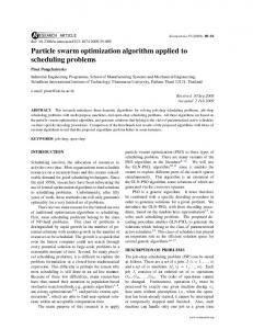
to be having a hard time capturing pieces, which was straightforward at the beginning of the second phase. One way we intend to solve this problem, in future work, is by explicitly steering the end game towards a good generalized strategy that would avoid this pitfall. Figure 1 shows how White’s weights for phase 1 have evolved over 200 epochs. Note that the initial values are random. For the first 50 epochs or so the weights are still being adjusted and fluctuate in the process, after which stagnation is reached, remaining relatively stable for the next 150 epochs. A complete set of evolved weights both for Black and White players is shown in Table I. These 15 values represent the weights for the combined features shown in vectors ~c1 and ~c2 in equations 2 and 3, respectively. The analysis of the values shown in the table, along with a sample game is shown in the next section, illustrating the effect of these values on the strategies and therefore on the outcome of the game. TABLE I S AMPLE W EIGHT V ECTORS FOR W HITE AND B LACK

3 2 2 (B

− 1) + 500 + 0.5 · r m + 500

where w represents the white and b the black pieces left on the board at the end of the game, m the number of moves made in that game, r is the result of the game (1 if Black won, -1 if White won or 0 if the game resulted in a draw), B the board size and P the total number of pieces a player has at the beginning of the game (24 in this case). The function produces a negative score if white has more pieces and vice versa for black. The term 32 (B 2 − 1) represents the minimum number of moves that can be made in order to win the game; the constant 500 is used to dilute the effect of the number of moves in the equation. A factor of 0.5 is added to or subtracted from the score of a game that didn’t result in a draw to reward the players for actually ending the game, instead of settling for a large difference in pieces by the end of the game. To sum up, each score depends on whether anyone won, the number of pieces left at the end and the number of moves. The large number of games were executed on a 14-processor cluster of Intel Zeon 2.2 GHz processors, with 512 MB of RAM on each processor. Each run of 200 iterations took a run-time of approximately 8 days. In previous work [1], the White population displayed a general tendency to play towards a draw. This is one of the reasons why we migrated to a larger board. The problem we now face is the greater sophistication of the game. On a 7 × 7 board, more games overall tend to lead to a draw, for different reasons, however. Once there is more free space on the board, the players have difficulty planning ahead in order to capture their opponents’ pieces. This is because of the reduction in depth that is applied to the minimax algorithm in order to conserve efficiency towards the end of the game when the average branching factor is at its highest. This tendency can be observed in the sample game in the following section. Although it is relatively easy for a human player to finish the game, the digital players seem

Weight 1 2 3 4 5 6 7 8 9 10 11 12 13 14 15

White 1.358074 0.301910 0.668130 0.086753 0.361836 0.361181 1.335093 0.529828 0.539433 0.169001 0.176832 0.357456 0.389927 0.516087 0.454301

Black 1.209082 0.196217 0.721942 0.171628 0.127716 0.230659 1.985006 0.009885 0.158170 0.114103 0.458611 0.740123 1.00919 0.103386 0.698025

Description beginning of phase 2 mass dist., encapsulation mass distance clustering corners + borders corners - borders material black clustering white clustering mass dist., encapsul. bl. clustering, encapsul. wh. clustering, encapsul. mass distance corners + borders corners - borders

Phase 1

2

The source code for the present version of the program is publicly available at the following URL: http://www.cs.aucegypt.edu/∼abdelbar/seega.html VI. A S AMPLE G AME This section shows a game as carried out on the game engine between two particles after 157 epochs, one from the White and one from the Black swarm, each with its own weight vector, whose values are listed in Table I. It is recommended that the reader refer to the table in order to fully understand the behavior of the players during the game. Below is a list of the moves made throughout the game: a white or a black circle signifies whose turn it is; one coordinate is given in the first phase of the game, which represents the position in which the disk was placed; both source and destination coordinates are given for phase two. The first board illustration (figure 2) shows the board at the end of stage one of the game. The strategies the players are following are already quite obvious. The white player seems to be concentrating more on defense, since it first tries to occupy the corners. Both players are less

1.2 1

w1

0.8 weight

0.6 0.4

w5 w3w2 w4

0.2

w6 0

100

200

300

400

500

iteration

Fig. 1.

A White particle’s feature weights for phase one

concerned with clustering their pieces in the first phase (weight 4), but have a lot of weight assigned to their fate at the beginning of the second phase (weight 1). It is noticeable, for example, that Black has tried to ensure that it makes the first few captures of the game and immediately captures 4 white pieces at the beginning of phase two. The distance in center of mass also plays an important role for both players. 1: ◦ d6, 5: ◦ b4, 9: ◦ e6, 13: ◦ a1, 17: ◦ a7, 21: ◦ c1, 25: ◦ d3, 29: ◦ b2, 33: ◦ c6, 37: ◦ a2, 41: ◦ c7, 45: ◦ a4,

2: • d2, 6: • e2, 10: • e1, 14: • f1, 18: • c2, 22: • c3, 26: • c4, 30: • f5, 34: • f6, 38: • b5, 42: • a3, 46: • a6,

3: ◦ d1, 7: ◦ g1, 11: ◦ g7, 15: ◦ b3, 19: ◦ e3, 23: ◦ d5, 27: ◦ b1, 31: ◦ d7, 35: ◦ e7, 39: ◦ f7, 43: ◦ b6, 47: ◦ e4,

4: • f4, 8: • f3, 12: • f2, 16: • g2, 20: • g3, 24: • g4, 28: • e5, 32: • c5, 36: • g5, 40: • g6, 44: • a5, 48: • b7,

7 6 5 4 3 2 1 a

b Fig. 2.

c

d

e

f

g

End of Phase One

The next moves are displayed below. Although Black is in the lead and is eating away at White’s pieces, it is

missing some relatively simple captures that White is taking advantage of. An interesting result of the co-evolutionary generation of the two players is how Black has put a really high value on clustering and encapsulation during the second phase (weight 11 and 12), while White has assigned it a value close to 0. And although both players should be concerned with material, Black has assigned a much higher value to the material weight (weight 7). On the other hand, White is more occupied with defense strategies, such as claiming corners and borders (see Table I). 49: • c4-d4, 53: ◦ d5-c5, 57: ◦ c6-c5, 61: ◦ d7-c7, 65: • f5-e5, 69: ◦ c7-b7, 73: ◦ f7-e7, 77: ◦ c5-d5, 81: ◦ c6-d6, 85: • e4-d4, 89: ◦ d5-e5, 93: • e3-d3, 97: ◦ d7-e7, 101: ◦ e5-f5, 105: • f7-g7, 109: • g4-g5, 113: • d6-c6, 117: • g5-g4, 121: • c6-b6, 125: • d3-c3, 129: ◦ c1-b1, 133: ◦ e6-e5, 137: ◦ d5-d4, 141: ◦ d3-c3, 145: ◦ b3-b2, 149: ◦ f7-g7, 153: • c1-c2, 157: • c1-c2,

50: • c3-d3, 54: • c3-b3, 58: • f3-e3, 62: ◦ d6-d7, 66: ◦ e7-e6, 70: • e3-e4, 74: • f5-e5, 78: ◦ d5-d4, 82: • e4-e3, 86: ◦ d6-d5, 90: ◦ e7-e6, 94: ◦ c3-b3, 98: • c5-c6, 102: • f6-f7, 106: ◦ b7-b6, 110: ◦ g6-g7, 114: • a3-b3, 118: ◦ b2-b3, 122: ◦ c1-c2, 126: • e1-d1, 130: • d1-d2, 134: • e4-d4, 138: • f1-e1, 142: • c2-c1, 146: • f4-e4, 150: • b4-b3, 154: ◦ g6-g7, 158: ◦ g6-g7,

51: • d3-c3, 55: • d4-d5, 59: ◦ c7-c6, 63: • d5-d6, 67: ◦ e6-d6, 71: ◦ c6-c5, 75: ◦ d6-c6, 79: • d2-d3, 83: ◦ c1-d1, 87: • e5-e4, 91: • f3-e3, 95: • c4-c3, 99: • c6-d6, 103: ◦ f5-g5, 107: • g7-f7, 111: ◦ g7-g6, 115: ◦ g6-g7, 119: • e5-e4, 123: • c4-d4, 127: ◦ b1-c1, 131: ◦ e7-e6, 135: ◦ e5-d5, 139: ◦ d4-d3, 143: ◦ b2-b3, 147: ◦ g7-f7, 151: • g4-f4, 155: • c2-c1, 159: • c2-c1,

52: • c5-c4, 56: • b3-b4, 60: • g3-f3, 64: • e5-d5, 68: • g5-f5, 72: • e5-e6, 76: • d5-d6, 80: ◦ d1-d2, 84: • e3-e4, 88: ◦ d2-d3, 92: ◦ d3-c3, 96: • b5-c5, 100: • c3-c4, 104: ◦ g7-g6, 108: ◦ g5-f5, 112: • e4-e5, 116: • b3-a3, 120: ◦ d1-c1, 124: ◦ c2-b2, 128: • c3-c2, 132: • d4-c4, 136: • d4-e4, 140: • e1-f1, 144: • e4-d4, 148: • d2-d3, 152: ◦ g7-g6, 156: ◦ g7-g6, 160: ◦ g7-g6,

Seega. Although the performance of the program seems to be improving, there still remains a lot to be done, especially with the larger board. The game has become much more sophisticated. Not only is more work needed on analyzing features and developing new ones, a whole new module needs to be added to the game engine to drive the end-game. At the moment, towards the end of the game, when the board becomes empty, look-ahead is not sufficient for the players to recognize their potential in winning the game, which is a trivial problem for any human player. We have avoided this problem in this paper by scoring a game even if it results in a draw. Essentially, we are cutting the game short and scoring it anyway. In the future, however, we will need a more sophisticated end-game engine.

7 6 5 4 3 2 1 a

b

Fig. 3.

c

d

e

f

g

Mid-game (after 120 moves)

R EFERENCES 161: 165: 169: 173: 177: 181: 185: 189:

• • • • • • • •

d3-d2, c2-d2, c1-d1, c2-d2, c2-d2, c1-c2, c3-c4, b5-b6,

162: ◦ g6-g7, 166: ◦ g6-g7, 170: ◦ g6-g7, 174: ◦ g6-g7, 178: ◦ g6-g5, 182: ◦ g6-g7, 186: ◦ g6-g7, 190: ◦ g6-g7

163: • d2-c2, 167: • d2-c2, 171: • d1-c1, 175: • d2-c2, 179: • c4-b4, 183: • c2-c3, 187: • b6-b5,

164: 168: 172: 176: 180: 184: 188:

◦ ◦ ◦ ◦ ◦ ◦ ◦

g7-g6, g7-g6, g7-g6, g7-g6, g5-g6, g7-g6, g7-g6,

7 6 5 4 3 2 1 a

b Fig. 4.

c

d

e

f

g

Game Over: Draw!

This has not had much implication on the game, since the problems at the end of the game still remain. Towards the end of the game, it seems to us as if Black has given up the fight and is moving around the board aimlessly, although it is simple for any human spectator to see how the game could be won (see fig 4). This game is a clear example of the problems we are currently facing with the end-game, which we hope to tackle in future work. Ideas for solutions are discussed in the next section. VII. C ONCLUSIONS AND F UTURE W ORK D IRECTIONS This paper continues on our attempt at developing a PSObased game engine for the ancient Egyptian board game

[1] A.M. Abdelbar, S. Ragab and S. Mitri. “Applying Co-evolutionary Particle Swarm Optimization to the Egypt Board Game Seega” Proceedings CEC-03 Workshop on Genetic Programming, pp. 9–15, 2003. [2] A.M. Abdelbar, and G. Tagliarini, “Using neural network learning in an Othello evaluation function,” Journal of Experimental and Theoretical Artificial Intelligence, vol. 10, pp. 217–229, 1998. [3] K.-F. Lee, and S. Mahajan, “The development of a world-class Othello program,” Artificial Intelligence, vol. 43, pp. 21–36, 1990. [4] Y. Shi, and R.A. Krohling, “Co-evolutionary particle swarm optimization to solve min-max problems,” In Proceedings IEEE Congress on Evolutionary Computation, 2002. [5] J. Kennedy, and R.C. Eberhart, “Particle swarm optimization,” In Proceedings IEEE International Conference on Neural Networks, vol. IV, pp. 1942–1948, 1995. [6] R.C. Eberhart, and J. Kennedy, “A new optimizer using particle swarm theory,” In Proceedings International Symposium on Micro Machine and Human Science, pp. 39-43, 1995. [7] J. Kennedy, and R. C. Eberhart, Swarm Intelligence, Morgan Kaufmann, San Francisco, 2001. [8] H. J. Van Den Herik, J. W. H. M. Uiterwijk, and J. Van Rijswijck, “Games solved: now and in the future,” Artificial Intelligence, vol. 134, pp. 277–311, 2002. [9] M. Campbell, A. J. Hoane, Jr., and F. Hsu, ‘ ‘Deep Blue,” Artificial Intelligence, vol. 134, pp. 57–83, 2002. [10] M. M¨uller, “Computer Go,” Artificial Intelligence, vol. 134, pp. 145– 179, 2002. [11] M. Burmeister, and J. Wiles, “AI techniques used in computer Go,” In Proceedings Fourth Conference of the Australasian Cognitive Science Society, 1997. [12] M. Buro, “From simple features to sophisticated evaluation functions,” In Proceedings First International Conference on Computers and Games (CG-98), pp. 126–145, 1998. [13] A. L. Samuel, “Some studies in machine learning using the game of checkers,” IBM Journal of Research and Development, vol. 44, No. 1/2, pp. 207–226, 2000. [14] M. Løvbjerg, T. K. Rasmussen, and T. Krink, “Hybrid particle swarm optimiser with breeding and subpopulations,” In Proceedings Third Genetic and Evolutionary Computation Conference (GECCO-01), vol. 1, pp. 469–476, 2001. [15] M. A. Potter, and K. A. De Jong, “A cooperative coevolutionary approach to function optimization,” In Proceedings Third Conference on Parallel Problem Solving from Nature, pp 249–257, 1994. [16] G. Tesauro, “TD-Gammon, a self-teaching backgammon program, achieves master-level play,” Neural Computation, vol. 6, pp. 215–219, 1994. [17] R. E. Korf, “Artificial Intelligence Search Algorithms,” In Algorithms and Theory of Computation Handbook, CRC Press, 1999. [18] A. G. Barto, R. S. Sutton, and C. W. Anderson, “Neuronlike adaptive elements that can solve difficult learning control problems,” 834–846, Sept./Oct. 1983.