A.4 Installing on Mac OS . . . . . . . . . . . . . . . . . . . . . . . . . 11. 1 Purpose. The COmparison of Continuous Optimizers (COCO) software1 is a benchmark- ing software to ... sulted in thirty-eight accepted workshop papers presenting results of state-of-.
COCO (COmparing Continuous Optimizers) Software: User Documentation Steffen Finck∗ and Raymond Ros† compiled March 22, 2010
Contents 1 Purpose
1
2 Experimental Framework Software 2.1 Running Experiments in C . . . . . . . . . . . . . . . . . . . . . 2.2 Running Experiments in Java . . . . . . . . . . . . . . . . . . . .
2 3 3
3 Post-Processing the Experimental Data 3.1 Using the bbob pproc Package . . . . . . . . . . . . . . . . . . . . 3.2 Comparison of Algorithms . . . . . . . . . . . . . . . . . . . . . .
4 7 7
4 Generating a Paper
8
A Installing bbob pproc A.1 Downloading the Packages A.2 Installing on Linux . . . . A.3 Installing on Windows . . A.4 Installing on Mac OS . . .
1
. . . .
. . . .
. . . .
. . . .
. . . .
. . . .
. . . .
. . . .
. . . .
. . . .
. . . .
. . . .
. . . .
. . . .
. . . .
. . . .
. . . .
. . . .
. . . .
. . . .
. . . .
. . . .
10 10 11 11 11
Purpose
The COmparison of Continuous Optimizers (COCO) software1 is a benchmarking software to render easier experiments in the field of continuous optimization. A post-processing Python package generates tables and figures to be included in a research paper template presenting all results. The COCO software was used for the GECCO 2009 workshop named BlackBox Optimization Benchmarking (BBOB-2009). The efforts of BBOB-2009 resulted in thirty-eight accepted workshop papers presenting results of state-ofthe-art algorithms. ∗ SF is with the Research Center PPE, University of Applied Sciene Vorarlberg, Hochschulstrasse 1, 6850 Dornbirn, Austria † RR is with the TAO Team of INRIA Saclay–ˆ Ile-de-France at the LRI, Universit´ e-Paris Sud, 91405 Orsay cedex, France 1 Available at http://coco.gforge.inria.fr
1
The same efforts will be pursued for the workshop BBOB-20102 to be held during GECCO 20103 . The COCO software provides: 1. a single generic function interface fgeneric to the benchmark functions of BBOB-2010, coded in Matlab/Gnu Octave and C, 2. Java Native Interface classes to use fgeneric in Java, 3. the Python post-processing module bbob pproc, 4. LATEX templates to generate papers, and 5. the corresponding documentation. The practitioner in BBO who wants to benchmark one or many algorithms on the BBOB-2010 testbeds has to download COCO, interface the algorithms to call the test functions in the testbed and use the post-processing tools. The most substantial part is to render the considered algorithms compatible with our software implementation. We describe the different steps for obtaining a complete workshop paper for an algorithm, thus allowing us to present the architecture of COCO. We also present additional facilities implemented for the comparison of the results of the many algorithms submitted. Section 2 presents the experimental framework software used to generate benchmarking data. Section 3 describes the post-processing facilities of COCO, namely the Python package bbob pproc. Section 4 briefly describes the process of compiling a paper regrouping all the post-processed results.
2
Experimental Framework Software
The experimental framework software mainly consists in the implementation of the methodology presented in [2]. The software is centered on the interface function, fgeneric. We describe the format of the output data files and the content of the files as they are written by fgeneric. These files are to be analysed with the provided post-processing tools that are described in Section 3. To display an example of the use of fgeneric, we provide two example scripts. Executing the Matlab scripts provided in Listings 2 and 3 results in testing an algorithm —MY OPTIMIZER in the examples, see Listing 1— on the noiseless testbed of BBOB-2010 and displaying measures of the time complexity of an algorithm respectively. In Listing 2, lines 6 to 10 set variables used by fgeneric. The whole set of experiment on the noiseless testbed is done by looping over the lines 18 to 36. The function fgeneric outputs the results of the experiments, also it provides a single interface to any of the test functions of the BBOB-2010 testbeds. Once fgeneric is loaded into memory, the initialization process, see line 21 in Listing 2, sets all variables internal to fgeneric: the test function considered, the instance considered, the output directory. Later calls to fgeneric evaluate the chosen test 2 http://coco.gforge.inria.fr/doku.php?id=bbob-2010
3 http://www.sigevo.org/gecco-2010/workshops.html#bbob
2
Listing 1: MY OPTIMIZER.m: Monte Carlo search in Matlab. At each iteration, 200 points are sampled and stored in a matrix of size DIM × 200 so as to reduce loops and function calls within Matlab and therefore improve its efficiency 1 2 3 4 5 6 7 8 9 10 11 12 13 14 15 16
function MY_OPTIMIZER(FUN, DIM, ftarget, maxfunevals) % MY_OPTIMIZER(FUN, DIM, ftarget, maxfunevals) % samples new points uniformly randomly in [-5,5]^DIM % and evaluates them on FUN until ftarget of maxfunevals % is reached, or until 1e8 * DIM fevals are conducted. % Relies on FUN to keep track of the best point. maxfunevals = min(1e8 * DIM, maxfunevals); popsize = min(maxfunevals, 200); for iter = 1:ceil(maxfunevals/popsize) feval(FUN, 10 * rand(DIM, popsize) - 5); if feval(FUN, ’fbest’) < ftarget % task achieved break; end % if useful, modify more options here for next start end
function at the point ~x given as input argument, see line 11 of Listing 1. Necessary finalization operations are effected by using the command fgeneric(’finalize’) in Matlab, see line 31 in Listing 2. In Listing 2, the function f8 is tested in 2, 3, 5, 10, 20, and 40-D. The while loop from line 15 to 18 make the runs last thirty seconds.
2.1
Running Experiments in C
The interface to fgeneric differs from the MATLAB example given in [2], we provide in Listing 4 the equivalent example script in C. A specific folder structure is needed for running an experiment. While creating the folder structure was handled by running fgeneric in Matlab, this is not the case using the C code. This folder structure can be obtained by un-tarring the archive createfolders.tar.gz and renaming the output folder or alternatively by executing the Python module createfolders before executing any experiment program. Make sure createfolders.py is in your current working directory and from the command-line simply do: python createfolders.py PUT_MY_BBOB_DATA_PATH Calls to fgeneric specified by a string first argument in MATLAB, are replaced by fgeneric string in C, e.g. fgeneric(’ftarget’) is replaced with fgeneric ftarget. Also, the generic call to fgeneric(X) to evaluate candidate vectors is replaced by fgeneric evaluate(double * X) for a single vector and fgeneric evaluate vector(double * XX, unsigned int np, double * result) for an array of vectors where XX is the concatenation of the np candidate vectors and result is an array of size np which contains the resulting function values.
2.2
Running Experiments in Java
The class JNIfgeneric implements an interface for using the C-implementation of fgeneric. Methods fgeneric string in C are replaced by JNIfgeneric.string, 3
Listing 2: exampleexperiment.m: script for benchmarking MY OPTIMIZER, see Listing 1, for BBOB-2010 on the noiseless function testbed in Matlab/Gnu Octave 1 2 3 4 5 6 7 8 9 10 11 12 13 14 15 16 17 18 19 20 21 22 23 24 25 26 27 28 29 30 31 32 33 34 35 36
% % % %
runs an entire experiment for benchmarking MY_OPTIMIZER on the noise-free testbed. fgeneric.m and benchmarks.m must be in the path of Matlab/Octave CAPITALIZATION indicates code adaptations to be made
addpath(’PUT_PATH_TO_BBOB/matlab’); % should point to fgeneric.m etc. datapath = ’PUT_MY_BBOB_DATA_PATH’; % different folder for each experiment opt.algName = ’PUT ALGORITHM NAME’; opt.comments = ’PUT MORE DETAILED INFORMATION, PARAMETER SETTINGS ETC’; maxfunevals = ’20 * dim’; % SHORT EXPERIMENT, takes overall three minutes more off;
% in octave pagination is on by default
t0 = clock; rand(’state’, sum(100 * t0)); % initialises the pseudo-random generator % in MY_OPTIMIZER for dim = [2,3,5,10,20,40] % small dimensions first, for CPU reasons for ifun = benchmarks(’FunctionIndices’) % or benchmarksnoisy(...) for iinstance = [1:15] % Instances 1 to 15 fgeneric(’initialize’, ifun, iinstance, datapath, opt); MY_OPTIMIZER(’fgeneric’, dim, fgeneric(’ftarget’), eval(maxfunevals)); disp(sprintf([’ f%d in %d-D, instance %d: FEs=%d,’ ... ’ fbest-ftarget=%.4e, elapsed time [h]: %.2f’], ... ifun, dim, iinstance, ... fgeneric(’evaluations’), ... fgeneric(’fbest’) - fgeneric(’ftarget’), ... etime(clock, t0)/60/60)); fgeneric(’finalize’); end disp([’ date and time: ’ num2str(clock, ’ %.0f’)]); end disp(sprintf(’---- dimension %d-D done ----’, dim)); end
except for the initialization JNIfgeneric.initBBOB(. . . ) and finalization JNIfgeneric.exitBBOB().
3
Post-Processing the Experimental Data
The Python post-processing tool, called bbob pproc in BBOB-2010 generates image files and LATEX tables from the raw experimental data obtained as described previously in Section 2. The entire post-processing tool requires that Python is installed on your machine. The minimal software requirements for using the post-processing tool are Python (2.5.2), Matplotlib (0.91.2) and Numpy (1.0.4). The installation of the software is described in Appendix A.
4
Listing 3: exampletiming.m: script for measuring the time complexity of MY OPTIMIZER, see Listing 1, for BBOB-2010 in Matlab/Gnu Octave 1 2 3 4 5 6 7 8 9 10 11 12 13 14 15 16 17 18 19 20 21 22 23 24 25 26
% runs the timing experiment for MY_OPTIMIZER. fgeneric.m % and benchmarks.m must be in the path of MATLAB/Octave addpath(’PUT_PATH_TO_BBOB/matlab’); more off;
% should point to fgeneric.m etc.
% in octave pagination is on by default
timings = []; runs = []; dims = []; for dim = [2,3,5,10,20,40] nbrun = 0; ftarget = fgeneric(’initialize’, 8, 1, ’tmp’); tic; while toc < 30 % at least 30 seconds MY_OPTIMIZER(@fgeneric, dim, ftarget, 1e5); % adjust maxfunevals nbrun = nbrun + 1; end % while timings(end+1) = toc / fgeneric(’evaluations’); dims(end+1) = dim; % not really needed runs(end+1) = nbrun; % not really needed fgeneric(’finalize’); disp([[’Dimensions:’ sprintf(’ %11d ’, dims)]; ... [’ runs:’ sprintf(’ %11d ’, runs)]; ... [’ times [s]:’ sprintf(’ %11.1e ’, timings)]]); end
Overview of the bbob pproc Package We present here the content of the latest version of the bbob pproc package (version 10.0). run.py is the main interface of the package that calls the different routines listed below, pproc.py defines the classes DataSetList and DataSet which are the main data structures that we use to gather the experimental raw data, ppfigdim.py, pptex.py, pprldistr.py are used to produce figures and tables that we describe further down, readalign.py, bootstrap.py contain routines for the post-processing of the raw experimental data, dataoutput.py contain routine to output instances of DataSet in Pythonformatted data files, bbob pproc.compall is a sub-package which contains modules for the comparison of the performances of algorithms, routines in this package can be called using the interface of runcompall.py, bbob pproc.comp2 is a sub-package which contains modules for the comparison of the performances of two algorithms, routines in this package can be called using the interface of runcomp2.py. 5
Listing 4: exampleexperiment.c: script for benchmarking MY OPTIMIZER, for BBOB-2010 on the noiseless function testbed in C 1 2 3 4 5 6 7 8 9 10 11 12 13 14 15 16 17 18 19 20 21 22 23 24 25 26 27 28 29 30 31 32 33 34 35 36 37 38 39 40 41 42 43 44 45 46 47 48 49 50 51 52 53 54 55
/*runs an entire experiment benchmarking MY_OPTIMIZER on the noise-free testbed*/ #include #include #include #include #include
"bbobStructures.h" /* Include all declarations for BBOB calls */
/* include all declarations for your own optimizer here */ void MY_OPTIMIZER(double(*fitnessfunction)(double*), unsigned int dim, double ftarget, unsigned int maxfunevals); int main() { unsigned int dim[6] = {2, 3, 5, 10, 20, 40}; unsigned int idx_dim, ifun, instance; clock_t t0 = clock(); time_t Tval; ParamStruct params = fgeneric_getDefaultPARAMS(); srand(time(NULL)); /* used by MY_OPTIMIZER */ strcpy(params.dataPath, "PUT_MY_BBOB_DATA_PATH"); /* please run ’python createfolders.py PUT_MY_BBOB_DATA_PATH’ beforehand */ strcpy(params.algName, "PUT ALGORITHM NAME"); strcpy(params.comments, "PUT MORE DETAILED INFORMATION, SETTINGS ETC"); for (idx_dim = 0; idx_dim < 6; idx_dim++) { /*Function indices are from 1 to 24 (noiseless) or from 101 to 130 (noisy)*/ for (ifun = 1; ifun >> import bbob_pproc >>> bbob_pproc.main(’DATAPATH’) This first command loads bbob pproc into memory and requires that the path to the package is in the Python search path. The resulting ppdata folder now contains a number of TEX, eps, png files. Additional help for the bbob pproc package can be obtained by executing the following command in a shell: python path_to_postproc_code/bbob_pproc/run.py -h In particular, this command describes the additional options for the execution of the post-processing. The code documentation can be found in the folder path to postproc code/pydoc within the provided software package.
3.2
Comparison of Algorithms
The sub-package bbob pproc.compall and bbob pproc.comp2 (v10.0) from bbob pproc provide facilities for the generation of tables and figures comparing the performances of algorithms tested using COCO. The post-processing works with data folders as input argument, with each folder corresponding to the data of an algorithm. Supposing you have the folders ALG1, ALG2 and ALG3 containing the data of algorithms ALG1, ALG2 and ALG3, you will need to execute from the command line: python path_to_postproc_code/bbob_pproc/runcompall.py ALG1 ALG2 ALG3 This assumes the folders ALG1, ALG2 and ALG3 are in the current working directory. In this case, the folders contain a number of files with the pickle extension which contain Python-formatted data or the raw experiment data with the info, dat and tdat extensions. Running the aforementioned command will generate the folder cmpalldata containing comparison figures and tables. Outputs appropriate to the comparison of only two algorithms can be obtained using bbob pproc.comp2 by executing from the command line: 4 The
package can be obtained from http://coco.gforge.inria.fr/doku.php?id= bbob-2010. 5 Note that in Windows the path separator ’\’ must be used instead of ’/’
7
python path_to_postproc_code/bbob_pproc/runcomp2.py ALG0 ALG1 This assumes the folders ALG0 and ALG1 are in the current working directory. Running the aforementioned command will generate the folder cmp2data containing the comparison figures. To run the post-processing from a Python shell, the following commands need to be executed: >>> from bbob_pproc import runcompall >>> bbob_pproc.runcompall.main(’ALG1 ALG2 ALG3’.split()) or: >>> from bbob_pproc import runcomp2 >>> bbob_pproc.runcomp2.main(’ALG0 ALG1’.split()) The from. . . import. . . command loads package into memory and requires that the path to the package is in the Python search path. Call to the main method runs the whole post-processing script.
4
Generating a Paper
templateBBOBarticle.tex and templateBBOBnoisyarticle.tex are the template LATEX files that include all the figures and tables presenting the result of an algorithm on the noiseless and noisy testbeds of BBOB-2010. If compiled correctly using LATEX, it generates documents collecting and organizing the output from bbob pproc. Each of the templates has a given page organization optimized for the presentation of the results on each testbed. To compile a document, one needs: 1. to have a working LATEX distribution6 , 2. to be in the correct working directory (containing the folder ppdata that includes all the output from the bbob pproc), 3. that templateBBOBarticle.tex7 , bbob.bib and sig-alternate.cls are in the working directory (all files are provided with the software), Then the following commands needs to be executed in a shell: latex templateBBOBarticle bibtex templateBBOBarticle latex templateBBOBarticle latex templateBBOBarticle The document templateBBOBarticle.dvi is then generated in the format required for a GECCO workshop paper. An example of the resulting template document obtained by compiling the LATEX template paper is provided here8 . 6 http://www.latex-project.org/ 7 or
templateBBOBnoisyarticle.tex for the noisy testbed of BBOB-2010. figures and tables show the data of the Monte Carlo search on the noiseless testbed of BBOB-2009 [1]. 8 The
8
1 Sphere
9
Black-Box Optimization Benchmarking Template for Noiseless Function Testbed
+1 +0
4
∗
-3
Forename Name
10
20
40
5 Linear slope
9
9 8 7 6 5 4 3 2 1 0
8
5 4
ABSTRACT
3 2
Categories and Subject Descriptors
1 0
G.1.6 [Numerical Analysis]: Optimization—global optimization, unconstrained optimization; F.2.1 [Analysis of Algorithms and Problem Complexity]: Numerical Algorithms and Problems
2
5
3
10
20
40
9 Rosenbrock rotated
9
3
2
2
1
1
40
2
7 Step-ellipsoid
9 8
8
7
7
12
6 5
5
4
4
5
10
20
40
10 Ellipsoid
1 0 2
5
3
10
20
40
2
11 Discus
9
7
5
4
4
3
13 Sharp ridge
9 8 7 6 5 4 3 2 1 0
7 6 5 4 3 2 1 0 2
5
3
10
20
40
17 Schaffer F7, condition 10
9
5
3
10
20
14 Sum of different powers
40
5
3
10
20
40
2
15 Rastrigin
9
5
3
10
20
40
18 Schaffer F7, condition 1000
8
8
7
7
6
6
5
5
4
4
1
2
5
3
10
20
40
2
19 Griewank-Rosenbrock F8F2
9
8
7
7
7
7
6
6
6
6
5
5
5
5
4
5
3
10
20
40
21 Gallagher 101 peaks
9
5
3
10
20
40
22 Gallagher 21 peaks
9
8
14
1 0 2
5
3
10
20
40
2
23 Katsuuras
9
8
7
2
1 0 2
8
7
7
7
6
6
6
5
5
5
4
4
4
3
3
2
10
20
40
24 Lunacek bi-Rastrigin
8
5
2
5
3
9
4 3
40
3
2
1 0 2
10
20 Schwefel x*sin(x)
4
3
2
1
6
4
3
2
5
3
9
8
3
20
2
0
8
0
10
16 Weierstrass
3
1 0
8
4
5
3
9
2
2
40
1 0 2
3
9
20
2
1 0 2
40
3
2
1
40
20
4
3
2
0 20
10
12 Bent cigar
8
6
10
5
3
9
8 7
5
40
2
1 0
5
3
20
3
2
3
10
8 Rosenbrock original
6
3
2
5
3
9
6
8
∗Camera-ready paper due April 17th.
20
7
9
[1] S. Finck, N. Hansen, R. Ros, and A. Auger. Real-parameter black-box optimization benchmarking 2009: Presentation of the noiseless functions. Technical Report 2009/20, Research Center PPE, 2009. [2] N. Hansen, A. Auger, S. Finck, and R. Ros. Real-parameter black-box optimization benchmarking 2009: Experimental setup. Technical Report RR-6828, INRIA, 2009. [3] N. Hansen, S. Finck, R. Ros, and A. Auger. Real-parameter black-box optimization benchmarking 2009: Noiseless functions definitions. Technical Report RR-6829, INRIA, 2009.
10
5
2
REFERENCES
0 5
3
6
1
RESULTS
6 Attractive sector
2
7
2
Results from experiments according to [2] on the benchmark functions given in [1, 3] are presented in Figures 1 and 2 and in Table 1.
40
5
0
Benchmarking, Black-box optimization, Evolutionary computation
20
6
3
Keywords
10
8
4
Algorithms
5
3
9
8
General Terms
+1 +0 -1
3
2
-2 -3
2
1
1
1
1
0
0
0
0
-5 -8
2
5
3
10
20
40
2
5
3
10
20
40
2
5
3
10
20
40
2
5
3
10
20
40
•
Figure 1: Expected Running Time (ERT, ) to reach fopt + ∆f and median number of function evaluations of successful trials (+), shown for ∆f = 10, 1, 10−1 , 10−2 , 10−3 , 10−5 , 10−8 (the exponent is given in the legend of f1 and f24 ) versus dimension in log-log presentation. The ERT(∆f ) equals to #FEs(∆f ) divided by the number of successful trials, where a trial is successful if fopt + ∆f was surpassed during the trial. The #FEs(∆f ) are the total number of function evaluations while fopt + ∆f was not surpassed during the trial from all respective trials (successful and unsuccessful), and fopt denotes the optimal function value. Crosses (×) indicate the total number of function evaluations #FEs(−∞). Numbers above ERT-symbols indicate the number of successful trials. Annotated numbers on the ordinate are decimal logarithms. Additional grid lines show linear and quadratic scaling.
Table 1: Shown are, for a given target difference to the optimal function value ∆f : the number of successful trials (#); the expected running time to surpass fopt + ∆f (ERT, see Figure 1); the 10%-tile and 90%-tile of the bootstrap distribution of ERT; the average number of function evaluations in successful trials or, if none was successful, as last entry the median number of function evaluations to reach the best function value (RTsucc ). If fopt + ∆f was never reached, figures in italics denote the best achieved ∆f -value of the median trial and the 10% and 90%-tile trial. Furthermore, N denotes the number of trials, and mFE denotes the maximum of number of function evaluations executed in one trial. See Figure 1 for the names of functions.
D=5
1.0
0.8
+1:6/24
-4:1/24 -8:0/24
0.6
0.4
0.2
0.0 0 1.0
0.8
2
3
4
5
6
0
2
4
log10 of FEvals / DIM f1-5
6
8
10
12
14
-8:0/24
0.4
0.0 0 1.0
16
log10 of Df / Dftarget
proportion of trials
proportion of trials
separable fcts
-4:0/5
0.4
0.2
0.8
2
3
4
5
6
0
2
4
log10 of FEvals / DIM f6-9
6
8
10
12
14
proportion of trials
proportion of trials
2
3
4
5
6
0
2
4
log10 of FEvals / DIM f10-14
6
8
10
12
14
0.8
2
4
6
8
10
12
14
16
log10 of Df / Dftarget
f1-5
1
2
3
4
5
6
0
2
4
log10 of FEvals / DIM f6-9
6
8
10
12
14
16
log10 of Df / Dftarget
-1:0/4 -4:0/4 -8:0/4
0.6
0.4
0.0 0 1.0
16
log10 of Df / Dftarget
f6-9
1
2
3
4
5
6
0
2
4
log10 of FEvals / DIM f10-14
6
8
10
12
14
16
log10 of Df / Dftarget
+1:1/5
proportion of trials
-1:1/5 -4:0/5 -8:0/5
0.6
0.4
0.8
-1:0/5 -4:0/5 -8:0/5
0.6
0.4
0.2
f10-14
1
2
3
4
5
6
0
2
4
log10 of FEvals / DIM f15-19
6
8
10
12
14
proportion of trials
0.6
0.4 +1:5/5 -1:0/5
-8:0/5 2
3
f15-19
4
5
6
0
2
4
log10 of FEvals / DIM f20-24
6
8
10
12
14
3
4
5
6
0
2
4
6
8
10
12
14
16
log10 of Df / Dftarget
-4:0/5 -8:0/5
0.4
f15-19
1
2
3
4
5
6
0
2
4
log10 of FEvals / DIM f20-24
6
8
10
12
14
16
log10 of Df / Dftarget
+1:2/5
+1:5/5 -1:2/5 -4:1/5
0.4
2
log10 of FEvals / DIM f15-19
-1:0/5
0.6
0.0 0 1.0
16
log10 of Df / Dftarget
0.8
0.6
0.8
0.2
-4:0/5
1
f10-14
1
+1:3/5
0.8
0.2
0.0 0 1.0
16
log10 of Df / Dftarget
proportion of trials
moderate fcts
0
0.2
f6-9
1
0.2
proportion of trials
6
0.4
+1:2/5
proportion of trials
ill-conditioned fcts
-4:0/4
0.2
-8:0/5
0.2
0.0 0
5
+1:0/4
-1:0/4
0.4
0.0 0 1.0
4
-8:0/5
0.0 0 1.0
16
log10 of Df / Dftarget
-8:0/4
0.0 0 1.0
3
-4:0/5
0.2
f1-5
1
0.6
0.8
2
log10 of FEvals / DIM f1-5
-1:0/5
0.6
+1:4/4
0.0 0 1.0
f1-24
1
+1:0/5
-1:1/5
-8:0/5
0.8
-4:0/24
0.2
f1-24
1
0.6
0.0 0 1.0
f1-24
-1:0/24
0.6
+1:4/5 0.8
D = 20
1.0
f1-24
-1:4/24 proportion of trials
proportion of trials
all functions
+1:20/24
multi-modal fcts
f 2 in 20-D, N=15, mFE=2.00 e7 # ERT 10% 90% RTsucc 0 12e+4 79e+3 15e+4 1.1 e7 . . . . . . . . . . . . . . . . . . . . . . . . . f 4 in 20-D, N=15, mFE=2.00 e7 # ERT 10% 90% RTsucc 0 33e+1 30e+1 35e+1 1.1 e7 . . . . . . . . . . . . . . . . . . . . . . . . . f 6 in 20-D, N=15, mFE=2.00 e7 # ERT 10% 90% RTsucc 0 48e+1 21e+1 46e+3 1.3 e7 . . . . . . . . . . . . . . . . . . . . . . . . . f 8 in 20-D, N=15, mFE=2.00 e7 # ERT 10% 90% RTsucc 0 80e+2 56e+2 10e+3 1.1 e7 . . . . . . . . . . . . . . . . . . . . . . . . . f 10 in 20-D, N=15, mFE=2.00 e7 # ERT 10% 90% RTsucc 0 11e+4 74e+3 17e+4 1.0 e7 . . . . . . . . . . . . . . . . . . . . . . . . . f 12 in 20-D, N=15, mFE=2.00 e7 # ERT 10% 90% RTsucc 0 28e+6 22e+6 35e+6 7.1 e6 . . . . . . . . . . . . . . . . . . . . . . . . . f 14 in 20-D, N=15, mFE=2.00 e7 # ERT 10% 90% RTsucc 15 3.4 e6 2.5 e6 4.4 e6 3.4 e6 0 80e–1 62e–1 91e–1 8.9 e6 . . . . . . . . . . . . . . . . . . . . f 16 in 20-D, N=15, mFE=2.00 e7 # ERT 10% 90% RTsucc 3 9.0 e7 4.9 e7 2.9 e8 1.0 e7 0 11e+0 95e–1 13e+0 1.1 e7 . . . . . . . . . . . . . . . . . . . . f 18 in 20-D, N=15, mFE=2.00 e7 # ERT 10% 90% RTsucc 0 18e+0 17e+0 20e+0 1.1 e7 . . . . . . . . . . . . . . . . . . . . . . . . . f 20 in 20-D, N=15, mFE=2.00 e7 # ERT 10% 90% RTsucc 0 15e+2 72e+1 27e+2 1.6 e7 . . . . . . . . . . . . . . . . . . . . . . . . . f 22 in 20-D, N=15, mFE=2.00 e7 # ERT 10% 90% RTsucc 1 3.0 e8 1.5 e8 >3 e8 1.7 e7 0 30e+0 18e+0 38e+0 1.0 e7 . . . . . . . . . . . . . . . . . . . . f 24 in 20-D, N=15, mFE=2.00 e7 # ERT 10% 90% RTsucc 0 26e+1 22e+1 27e+1 7.1 e6 . . . . . . . . . . . . . . . . . . . . . . . . .
proportion of trials
f 2 in 5-D, N=15, mFE=5.00 e6 ∆f # ERT 10% 90% RTsucc 10 0 11e+1 57e+0 22e+1 1.8 e6 1 . . . . . 1e−1 . . . . . 1e−3 . . . . . 1e−5 . . . . . 1e−8 . . . . . f 4 in 5-D, N=15, mFE=5.00 e6 ∆f # ERT 10% 90% RTsucc 10 5 1.3 e7 7.7 e6 2.3 e7 2.6 e6 1 0 12e+0 47e–1 16e+0 2.5 e6 1e−1 . . . . . 1e−3 . . . . . 1e−5 . . . . . 1e−8 . . . . . f 6 in 5-D, N=15, mFE=5.00 e6 ∆f # ERT 10% 90% RTsucc 10 15 3.5 e4 2.3 e4 4.7 e4 3.5 e4 1 5 1.2 e7 7.4 e6 2.3 e7 2.2 e6 1e−1 0 14e–1 73e–2 17e–1 2.5 e6 1e−3 . . . . . 1e−5 . . . . . 1e−8 . . . . . f 8 in 5-D, N=15, mFE=5.00 e6 ∆f # ERT 10% 90% RTsucc 10 15 1.5 e6 1.0 e6 2.0 e6 1.5 e6 1 0 64e–1 41e–1 90e–1 2.0 e6 1e−1 . . . . . 1e−3 . . . . . 1e−5 . . . . . 1e−8 . . . . . f 10 in 5-D, N=15, mFE=5.00 e6 ∆f # ERT 10% 90% RTsucc 10 0 10e+1 41e+0 20e+1 2.2 e6 1 . . . . . 1e−1 . . . . . 1e−3 . . . . . 1e−5 . . . . . 1e−8 . . . . . f 12 in 5-D, N=15, mFE=5.00 e6 ∆f # ERT 10% 90% RTsucc 10 0 19e+3 12e+3 29e+3 2.8 e6 1 . . . . . . . . . 1e−1 . 1e−3 . . . . . 1e−5 . . . . . . . . . 1e−8 . f 14 in 5-D, N=15, mFE=5.00 e6 ∆f # ERT 10% 90% RTsucc 10 15 1.2 e1 8.1 e0 1.6 e1 1.2 e1 1 15 4.1 e3 3.1 e3 5.1 e3 4.1 e3 1e−1 10 4.4 e6 2.9 e6 6.7 e6 1.9 e6 1e−3 0 93e–3 49e–3 14e–2 2.2 e6 1e−5 . . . . . . . . . 1e−8 . f 16 in 5-D, N=15, mFE=5.00 e6 ∆f # ERT 10% 90% RTsucc 10 15 4.3 e2 2.7 e2 6.0 e2 4.3 e2 1 15 3.1 e5 2.4 e5 4.0 e5 3.1 e5 1e−1 0 30e–2 17e–2 45e–2 2.8 e6 . . . . 1e−3 . 1e−5 . . . . . 1e−8 . . . . . f 18 in 5-D, N=15, mFE=5.00 e6 ∆f # ERT 10% 90% RTsucc 10 15 1.8 e3 1.0 e3 2.7 e3 1.8 e3 1 2 3.6 e7 1.7 e7 >7 e7 3.0 e6 1e−1 0 15e–1 95e–2 18e–1 2.5 e6 1e−3 . . . . . 1e−5 . . . . . 1e−8 . . . . . f 20 in 5-D, N=15, mFE=5.00 e6 ∆f # ERT 10% 90% RTsucc 10 15 4.6 e2 3.2 e2 6.0 e2 4.6 e2 1 8 7.9 e6 5.5 e6 1.3 e7 3.5 e6 1e−1 0 99e–2 86e–2 12e–1 3.2 e6 . . . . 1e−3 . 1e−5 . . . . . 1e−8 . . . . . f 22 in 5-D, N=15, mFE=5.00 e6 # ERT 10% 90% RTsucc ∆f 10 15 5.4 e2 3.3 e2 7.5 e2 5.4 e2 1 15 2.8 e4 2.2 e4 3.5 e4 2.8 e4 1e−1 15 3.7 e5 2.3 e5 5.1 e5 3.7 e5 1e−3 1 7.2 e7 3.4 e7 >7 e7 1.9 e6 1e−5 0 93e–4 13e–4 31e–3 3.5 e6 1e−8 . . . . . f 24 in 5-D, N=15, mFE=5.00 e6 ∆f # ERT 10% 90% RTsucc 10 10 4.8 e6 3.2 e6 7.2 e6 2.3 e6 1 0 96e–1 78e–1 12e+0 2.0 e6 1e−1 . . . . . 1e−3 . . . . . 1e−5 . . . . . 1e−8 . . . . .
weak structure fcts
Permission to make digital or hard copies of all or part of this work for personal or classroom use is granted without fee provided that copies are not made or distributed for profit or commercial advantage and that copies bear this notice and the full citation on the first page. To copy otherwise, to republish, to post on servers or to redistribute to lists, requires prior specific permission and/or a fee. GECCO’09, July 8–12, 2009, Montréal Québec, Canada. Copyright 2009 ACM 978-1-60558-505-5/09/07 ...$5.00.
f 1 in 20-D, N=15, mFE=2.00 e7 # ERT 10% 90% RTsucc 0 29e+0 27e+0 33e+0 1.0 e7 . . . . . . . . . . . . . . . . . . . . . . . . . f 3 in 20-D, N=15, mFE=2.00 e7 # ERT 10% 90% RTsucc 0 26e+1 23e+1 29e+1 7.1 e6 . . . . . . . . . . . . . . . . . . . . . . . . . f 5 in 20-D, N=15, mFE=2.00 e7 # ERT 10% 90% RTsucc 0 11e+1 97e+0 12e+1 1.0 e7 . . . . . . . . . . . . . . . . . . . . . . . . . f 7 in 20-D, N=15, mFE=2.00 e7 # ERT 10% 90% RTsucc 0 10e+1 68e+0 11e+1 7.1 e6 . . . . . . . . . . . . . . . . . . . . . . . . . f 9 in 20-D, N=15, mFE=2.00 e7 # ERT 10% 90% RTsucc 0 68e+2 54e+2 90e+2 1.1 e7 . . . . . . . . . . . . . . . . . . . . . . . . . f 11 in 20-D, N=15, mFE=2.00 e7 # ERT 10% 90% RTsucc 0 67e+0 48e+0 70e+0 1.1 e7 . . . . . . . . . . . . . . . . . . . . . . . . . f 13 in 20-D, N=15, mFE=2.00 e7 # ERT 10% 90% RTsucc 0 92e+1 83e+1 10e+2 8.9 e6 . . . . . . . . . . . . . . . . . . . . . . . . . f 15 in 20-D, N=15, mFE=2.00 e7 # ERT 10% 90% RTsucc 0 26e+1 23e+1 28e+1 8.9 e6 . . . . . . . . . . . . . . . . . . . . . . . . . f 17 in 20-D, N=15, mFE=2.00 e7 # ERT 10% 90% RTsucc 15 7.5 e3 5.4 e3 9.8 e3 7.5 e3 0 50e–1 43e–1 55e–1 7.1 e6 . . . . . . . . . . . . . . . . . . . . f 19 in 20-D, N=15, mFE=2.00 e7 # ERT 10% 90% RTsucc 15 5.9 e5 4.2 e5 7.6 e5 5.9 e5 0 78e–1 63e–1 82e–1 1.1 e7 . . . . . . . . . . . . . . . . . . . . f 21 in 20-D, N=15, mFE=2.00 e7 # ERT 10% 90% RTsucc 0 26e+0 21e+0 30e+0 1.0 e7 . . . . . . . . . . . . . . . . . . . . . . . . . f 23 in 20-D, N=15, mFE=2.00 e7 # ERT 10% 90% RTsucc 15 8.3 e0 5.8 e0 1.1 e1 8.3 e0 3 8.9 e7 4.9 e7 2.9 e8 9.4 e6 0 11e–1 87e–2 12e–1 1.3 e7 . . . . . . . . . . . . . . .
4
3
0 2
6
f 1 in 5-D, N=15, mFE=5.00 e6 ∆f # ERT 10% 90% RTsucc 10 15 8.2 e1 5.4 e1 1.1 e2 8.2 e1 1 15 2.0 e4 1.4 e4 2.7 e4 2.0 e4 1e−1 7 8.3 e6 5.4 e6 1.5 e7 2.5 e6 1e−3 0 10e–2 55e–3 15e–2 2.8 e6 1e−5 . . . . . 1e−8 . . . . . f 3 in 5-D, N=15, mFE=5.00 e6 ∆f # ERT 10% 90% RTsucc 10 10 4.8 e6 3.3 e6 7.4 e6 2.3 e6 1 0 83e–1 56e–1 11e+0 3.2 e6 1e−1 . . . . . 1e−3 . . . . . 1e−5 . . . . . 1e−8 . . . . . f 5 in 5-D, N=15, mFE=5.00 e6 ∆f # ERT 10% 90% RTsucc 10 15 4.3 e4 3.0 e4 5.8 e4 4.3 e4 1 0 37e–1 23e–1 42e–1 2.2 e6 1e−1 . . . . . 1e−3 . . . . . 1e−5 . . . . . 1e−8 . . . . . f 7 in 5-D, N=15, mFE=5.00 e6 ∆f # ERT 10% 90% RTsucc 10 15 9.1 e2 6.6 e2 1.2 e3 9.1 e2 1 15 3.9 e5 2.9 e5 5.0 e5 3.9 e5 1e−1 0 38e–2 20e–2 66e–2 2.2 e6 1e−3 . . . . . 1e−5 . . . . . 1e−8 . . . . . f 9 in 5-D, N=15, mFE=5.00 e6 ∆f # ERT 10% 90% RTsucc 10 15 1.4 e6 1.0 e6 1.8 e6 1.4 e6 1 0 58e–1 42e–1 89e–1 3.2 e6 1e−1 . . . . . 1e−3 . . . . . 1e−5 . . . . . 1e−8 . . . . . f 11 in 5-D, N=15, mFE=5.00 e6 ∆f # ERT 10% 90% RTsucc 10 15 1.0 e5 8.6 e4 1.2 e5 1.0 e5 1 3 2.2 e7 1.2 e7 7.2 e7 2.1 e6 2.0 e6 1e−1 0 11e–1 57e–2 24e–1 1e−3 . . . . . 1e−5 . . . . . . . . . 1e−8 . f 13 in 5-D, N=15, mFE=5.00 e6 ∆f # ERT 10% 90% RTsucc 10 0 30e+0 17e+0 45e+0 3.2 e6 1 . . . . . 1e−1 . . . . . 1e−3 . . . . . 1e−5 . . . . . . . . . 1e−8 . f 15 in 5-D, N=15, mFE=5.00 e6 ∆f # ERT 10% 90% RTsucc 10 13 3.5 e6 2.7 e6 4.6 e6 2.7 e6 1 0 83e–1 64e–1 11e+0 3.5 e6 1e−1 . . . . . . . . . 1e−3 . 1e−5 . . . . . 1e−8 . . . . . f 17 in 5-D, N=15, mFE=5.00 e6 ∆f # ERT 10% 90% RTsucc 10 15 2.1 e1 1.3 e1 2.9 e1 2.1 e1 1 15 1.8 e5 1.2 e5 2.4 e5 1.8 e5 1e−1 0 48e–2 39e–2 57e–2 2.5 e6 1e−3 . . . . . 1e−5 . . . . . 1e−8 . . . . . f 19 in 5-D, N=15, mFE=5.00 e6 ∆f # ERT 10% 90% RTsucc 10 15 3.8 e1 2.9 e1 4.7 e1 3.8 e1 1 15 1.4 e5 1.1 e5 1.7 e5 1.4 e5 1e−1 0 36e–2 27e–2 48e–2 2.2 e6 . . . . 1e−3 . 1e−5 . . . . . 1e−8 . . . . . f 21 in 5-D, N=15, mFE=5.00 e6 # ERT 10% 90% RTsucc ∆f 10 15 1.3 e2 8.8 e1 1.8 e2 1.3 e2 1 15 9.8 e3 6.6 e3 1.3 e4 9.8 e3 1e−1 15 4.5 e5 3.2 e5 5.9 e5 4.5 e5 1e−3 0 14e–3 36e–4 18e–3 2.8 e6 1e−5 . . . . . 1e−8 . . . . . f 23 in 5-D, N=15, mFE=5.00 e6 ∆f # ERT 10% 90% RTsucc 10 15 7.0 e0 5.5 e0 8.7 e0 7.0 e0 1 15 2.6 e4 2.0 e4 3.2 e4 2.6 e4 1e−1 0 38e–2 31e–2 43e–2 4.0 e6 1e−3 . . . . . 1e−5 . . . . . 1e−8 . . . . .
4
1 0
5
3
7
2.
5
-8 0 2
1.
7 6
5
2
-5
4 Skew Rastrigin-Bueche separable
8
7 6
5
3
-2
1
9
8
7 6
4
-1
2
3 Rastrigin separable
9
8
7
5
3
Draft version
2 Ellipsoid separable
9
8
6
0.8
-1:0/5 -4:0/5 -8:0/5
0.6
0.4
0.2
f20-24
1
2
3
4
log10 of FEvals / DIM
5
6
0
2
4
6
8
10
12
log10 of Df / Dftarget
14
16
0.0 0
f20-24
1
2
3
4
log10 of FEvals / DIM
5
6
0
2
4
6
8
10
12
14
16
log10 of Df / Dftarget
Figure 2: Empirical cumulative distribution functions (ECDFs), plotting the fraction of trials versus running time (left subplots) or versus ∆f (right subplots). The thick red line represents the best achieved results. Left subplots: ECDF of the running time (number of function evaluations), divided by search space dimension D, to fall below fopt + ∆f with ∆f = 10k , where k is the first value in the legend. Right subplots: ECDF of the best achieved ∆f divided by 10k (upper left lines in continuation of the left subplot), and best achieved ∆f divided by 10−8 for running times of D, 10 D, 100 D . . . function evaluations (from right to left cycling black-cyan-magenta). Top row: all functions; second row: separable functions; third row: misc. moderate functions; fourth row: ill-conditioned functions; fifth row: multi-modal functions with adequate structure; last row: multi-modal functions with weak structure. The legends indicate the number of functions that were solved in at least one trial. FEvals denotes number of function evaluations, D and DIM denote search space dimension, and ∆f and Df denote the difference to the optimal function value.
The participants of BBOB-2010 are expected to fill in the template with all of their information, the description of their algorithm and their parameter settings [2], their source code or a reference to it, their results on the timing experiment. The BibTEX file bbob.bib includes the references to the BBOB2010 experimental set-up and documentation.
Acknowledgments Steffen Finck was supported by the Austrian Science Fund (FWF) under grant P19069-N18. The BBOBies would like to acknowledge Miguel Nicolau for his insights and the help he has provided on the implementation of the C-code. The BBOBies would also like to acknowledge Mike Preuss for his implementation of the JNI for using the C-code in Java, and Petr Poˇs´ık for his help and feedback in the beta-tests.
References [1] Anne Auger and Raymond Ros. Benchmarking the pure random search on the BBOB-2009 testbed. In Franz Rothlauf, editor, GECCO (Companion), pages 2479–2484. ACM, 2009. [2] N. Hansen, A. Auger, S. Finck, and R. Ros. Real-parameter black-box optimization benchmarking 2010: Experimental setup. Technical Report RR-7215, INRIA, 2010.
Installing bbob pproc
A
The entire post-processing tool is written in Python and requires Python to be installed on your machine. The minimal software requirements for using the post-processing tool are Python (2.5.2), Matplotlib (0.91.2) and Numpy (1.0.4). In the following, we explain how to obtain and install the required software for different systems (Linux, Windows, Mac OS) and which steps you have to perform to run the post-processing on your data. While the bbob pproc source files are provided, you need to install Python and its libraries Matplotlib and Numpy. We recommend using Python 2.6 and not a higher version (3.0, 3.1) since the necessary libraries are not (yet) available and the code is not verified.
A.1
Downloading the Packages
For all operating systems the packages can be found at the following locations: • Python: http://www.python.org/download/releases/, • Numpy: http://sourceforge.net/projects/numpy/, • Matplotlib: http://sourceforge.net/projects/matplotlib/. We recommend the use of the latest versions of Matplotlib (0.99.1.2), Python (2.6.4) and Numpy (1.4.0). 10
A.2
Installing on Linux
In most common Linux distributions Python (not Numpy or Matplotlib) is already part of the installation. If not, use your favorite package manager to install Python (package name: python), Numpy (python-numpy) and Matplotlib (package name: python-matplotlib) and their dependencies. If your distribution and repositories are up-to-date, you should have at least Python (2.6.4), Matplotlib (0.99.0) and Numpy (1.3.0). Though those are not the most recent versions of each package, they meet the minimal software requirements to make the BBOB2010 software work. If needed, you can alternatively download sources and compile binaries. Python and the latest versions of Matplotlib and Numpy can be downloaded from the links in Section A.1. A dependency for the Linux version of Matplotlib is libpng, which can be obtained at http://www.libpng.org/. You then need to properly install the downloaded packages before you can use them. Please refer to the corresponding package installation pages.
A.3
Installing on Windows
For installing Python under Windows, please go to the Python link in Section A.1 and download python-2.6.4.msi. This file requires the Microsoft Installer, which is a part of Windows XP and later releases. If you don’t have the Microsoft Installer, there is a link for the download provided at the same page. After installing Python, it is recommended to first install Numpy and then Matplotlib. Both can be installed with the standard .exe files which are respectively • numpy-1.4.0-win32-superpack-python2.6.exe and, • matplotlib-0.99.1.win32-py2.6.exe. These files can be obtained from the provided SourceForge links in Section A.1.
A.4
Installing on Mac OS
Mac OS X comes with Python pre-installed, the version might be older than 2.6 though. It is recommended to upgrade Python by downloading and installing a newer version. To do this, if you have Mac OS X 10.3 and later you can download the disk image file python-2.6.4 macosx10.3.dmg containing universal binaries from the Python download page, see Section A.1. More information on the update of Python on Mac OS can be found at this location: http://www.python.org/download/mac/9 . Open the disk image and use the installer10 . You then need to download and install Numpy and Matplotlib from the SourceForge links listed in Sect A.1.
9 The discussion over IDLE for Leopard user (http://wiki.python.org/moin/MacPython/ Leopard) is not relevant for the use of bbob pproc package. 10 Following this step leave the pre-installed Python on the system and install the MacPython 2.6.4 distribution. MacPython contains a Python installation as well as some Mac-specific extras.
11