Cocoon bifurcation in three-dimensional reversible vector fields Freddy Dumortier Universiteit Hasselt Campus Diepenbeek Agoralaan-Gebouw D, B-3590, Diepenbeek, Belgium E-mail:
[email protected] Santiago Ib´an ˜ez∗ Department of Mathematics University of Oviedo Avda. Calvo Sotelo s/n, 33007 Oviedo, Spain E-mail:
[email protected] Hiroshi Kokubu† Department of Mathematics Kyoto University Kyoto 606-8502, Japan E-mail:
[email protected] Dedicated to Robert Roussarie for his sixtieth birthday September 19, 2005 ∗ †
Partially supported by the projects FICYT PB-EXP01-29 and MCT-02-BFM-00241. Partially supported by Grant-in-Aid for Scientific Research (No.14340055, No.
1
Abstract The cocoon bifurcation is a set of rich bifurcation phenomena numerically observed by Lau [17] in the Michelson system, a threedimensional ODE system describing travelling waves of the KuramotoSivashinsky equation. In this paper, we present an organizing center of the principal part of the cocoon bifurcation in more general terms in the setting of reversible vector fields on R3 . We prove that in a generic unfolding of an organizing center called the cusp-transverse heteroclinic chain, there is a cascade of heteroclinic bifurcations with increasing length close to the organizing center, which resembles the principal part of the cocoon bifurcation. We also study a heteroclinic cycle called the reversible Bykov cycle. Such a cycle is believed to occur in the Michelson system, as well as in a model equation of a Josephson Junction ([23]). We conjecture that a reversible Bykov cycle is, in its unfolding, an accumulation point of a sequence of cusp-transverse heteroclinic chains. As a first result in this direction, we show that a reversible Bykov cycle is an accumulation point of reversible generic saddle-node bifurcations of periodic orbits, the main ingredient of the cusp-transverse heteroclinic chain.
1
Introduction
There are a number of papers devoted to studying the dynamics and bifurcations of the following one-parameter family of vector fields on R3 (e.g. [5, 11, 12, 13, 17, 19, 20, 22, 24]): x˙ = y y˙ = z z˙ = c2 −
x2 2
(1.1) − y.
On one hand, this system appears as a part of the limit family of the unfolding of the nilpotent singularity of codimension three (see [5]) given by the following equations: x˙ = y y˙ = z (1.2) 2 z˙ = λ + µy + νz + x , 17340045), Ministry of Education, Science, Technology, Culture and Sports, Japan.
2
where (λ, µ, ν) ∈ S 2 . When ν = 0, λ ≤ 0 and µ < 0, a simple change of coordinates and a reparametrization transforms (1.2) into the family (1.1). On the other hand, the family (1.1), also called the Michelson system, appears as the equation for travelling wave solutions of a non-linear PDE called the Kuramoto-Sivashinsky equation in one-dimensional media: 1 ut + uxxxx + uxx + u2x = 0, 2
(t ≥ 0, x ∈ R).
See [12] or [20] for precise derivation of (1.1) from the PDE. Because of this reason, the system (1.1) has attracted much attention for research. Let us observe some basic properties of (1.1): • Since the divergence is identically zero, the family is volume-preserving. • The family is reversible, namely, it is invariant under the involution R : (x, y, z) 7→ (−x, y, −z) and the time reverse t 7→ −t. • For c > 0 there are only two equilibrium points at √ P± = (± 2c, 0, 0), both are of saddle-focus type with dim(W u (P+ )) = dim(W s (P− )) = 2. As was pointed out in [20], it follows from the results in [19] that for c large enough there is a unique transverse heteroclinic orbit connecting P+ and P− in (1.1) which is given by the intersection of the two-dimensional invariant manifolds, and the equilibrium points together with the heteroclinic orbit form the maximal bounded invariant set of the family (1.1). When the parameter c decreases, according to the numerical results in [17] and [20], the family exhibits an infinite sequence of heteroclinic bifurcations, each of which creates a pair of new transverse heteroclinic orbits. Again it follows from the numerical results in these papers that the sequence of heteroclinic bifurcations converges to c¯ ≈ 1.2662. For this value, there appears a saddle-node bifurcation that creates a periodic orbit γ∗ , symmetric under the involution R and intersecting with the y-axis, which is the fixed point subspace of R. According to [20], the parameter value c¯ seems corresponding to the largest value for which a periodic orbit exists. The sequence of bifurcations that appear before and after c = c¯ was studied by Lau [17] mainly using careful numerical simulation, and was called the “cocoon” bifurcation, because of the specific shape of the invariant manifolds controlling the process, see [17]. 3
The cascade of heteroclinic bifurcations, caused by the tangency of W u (P+ ) and W s (P− ), and accumulating from above to the parameter value c¯ ≈ 1.2662, has been numerically observed by Lau. Here we call it the “principal sequence” of Lau’s cocoon bifurcation. The goal of this paper is to study this principal sequence from a theoretical and more general point of view, and to explain its occurrence as a consequence of the presence of an organizing center. In order to state our main results precisely, we begin by stating some definitions. Let Xλ be a one-parameter family of vector fields on R3 having the following properties: (H1) Each of the vector fields Xλ is time-reversible with respect to the linear involution R with dim(Fix(R)) = 1, where Fix(R) stands for the fixed point subspace of R; (H2) There exist two hyperbolic equilibrium points P± 6∈ Fix(R) which are symmetric under the involution R and such that dim W u (P+ ) = dim W s (P− ) = 2. Remark 1.1 Without loss of generality, one can assume that the linear involution R in (H1) is given by the map (x, y, z) 7→ (−x, y, −z). Remark 1.2 We refer to [15] for a quite complete survey and an extensive bibliography about reversible dynamical systems in both continuous and discrete cases. Definition 1.3 Under the conditions (H1) and (H2), we say the family Xλ exhibits a cocooning cascade of heteroclinic tangencies centered at λ∗ , if there is a closed solid torus T with P± 6∈ T and a monotone infinite sequence of parameters λn converging to λ∗ , for which the corresponding vector field Xλn has a tangency of W u (P+ ) and W s (P− ) such that the heteroclinic tangency orbit intersects with T and has its length within T tending to infinity as n → ∞. Definition 1.4 A family of vector fields Xλ on R3 satisfying (H1) and (H2) is said to have a cusp-transverse heteroclinic chain at λ = λ0 , if the following three conditions hold: (C1) Xλ0 has a saddle-node periodic orbit γ∗ which is symmetric under the involution R. 4
(C2) The saddle-node periodic orbit γ∗ is generic and generically unfolded in Xλ under the reversibility with respect to R. (C3) W u (γ∗ ) and W s (P− ), as well as W s (γ∗ ) and W u (P+ ), intersect transversely, where W s (γ∗ ) and W u (γ∗ ) stand for the stable and unstable sets of the non-hyperbolic periodic orbit γ∗ . Note that, because of the reversibility, the saddle-node periodic orbit in (C1) must intersect with Fix(R) (see [15]). Our main result is the following: Theorem 1.5 Let Xλ be a smooth family of reversible vector fields on R3 with (H1) and (H2). Suppose at λ = λ0 the corresponding vector field Xλ0 has a cusp-transverse heteroclinic chain. Then the family Xλ exhibits a cocooning cascade of heteroclinic tangencies centered at λ0 . Remark 1.6 The name “cusp-transverse” comes from the fact that, under the genericity condition (C2), the Poincar´e map along the saddle-node periodic orbit has a fixed point whose stable and unstable sets form a cusp, see Figure 1 in Section 2, and by the condition (C3) they intersects the unstable and stable manifolds of the equilibrium points P± transversely. Under the bifurcation, the saddle-node periodic orbit will split into two periodic orbits for λ on one side of λ∗ , while no periodic orbit will be present near γ∗ for λ on the other side of λ∗ . The cocooning cascade occurs for the latter values of λ. Geometric structure of the cusp-transverse heteroclinic chain will become clear once the local structure of the saddle-node periodic orbit is studied in Section 2. See Figure 3 as representing a crucial part of the structure. Remark 1.7 We briefly illustrate how the generic saddle-node periodic orbit implies the cusp structure in the case of (1.1). The family (1.1) is reversible under the linear involution R : (x, y, z) 7→ (−x, y, −z) whose fixed point subspace is the y-axis, hence one-dimensional. Suppose at a parameter value λ = λ0 , there is a saddle-node periodic orbit γ which is invariant under R and hence intersects with the y-axis. Denote by Π the Poincar´e map along γ at a point p = (0, y0 , 0) in Fix(R). Notice that p is a fixed point of Π. Since the vector field is reversible, by choosing the (y, z)-plane as an invariant cross section under R, one sees that Π is also reversible, namely it is conjugate to its inverse by the restricted involution. In particular, the determinant of DΠ(p) at the fixed point p is equal to 1, because the Poincar´e map is 5
flow-defined, hence orientation preserving. Knowing that 1 is an eigenvalue of DΠ(p) as p is a saddle-node fixed point, we conclude that 1 is a double eigenvalue of DΠ(p). Moreover, we assume that the eigenvalue 1 is not semisimple, which is a generic condition under the presence of saddle-node. This fact is supported by a numerical result in Section 4 for (1.1). It follows that the linear part of Π is conjugate to the unipotent matrix µ ¶ 1 1 . (1.3) 0 1 In the analysis developed in Section 2, a reversible diffeomorphism with the unipotent linear part at a fixed point is studied through a nilpotent singularity of a planar reversible vector field. By using the blow up technique, we can show that the stable and unstable sets of the fixed point of Π indeed form a cusp structure. Remark 1.8 The description of “cocoon bifurcations” in Lau’s paper [17] is phenomenological, in the sense that a list of dynamical behaviors and their changes (bifurcations) with variation of the parameter c is given in relation to associated changes in the structure of numerically computed stable and unstable manifolds of equilibrium points. Our motivation was to treat these complex bifurcation phenomena by a general and solid mathematical manner. Theorem 1.5 says that at least a part of it, namely the accumulation of infinitely many heteroclinic tangency bifurcations, can be understood as a consequence of the presence of a cusp-transverse heteroclinic chain. Therefore one can understand that such a sequence of heteroclinic bifurcations in the description of Lau’s cocoon bifurcation is not a special bifurcation phenomenon which occurs only in the Michelson system. Indeed, it will be shown that the same phenomena indeed occurs in a different system. We believe that other part of the Lau’s cocoon bifurcations can also be understood from this point of view, but this will be the subject of future work. In order to rigorously show the existence of a cusp-transverse heteroclinic chain in a given family of vector fields, one must verify the conditions (C1C3), which is in general not easy by analytical methods and often requires numerical computation (see Section 4). However, we believe there is a bifurcation mechanism producing cusp-transverse heteroclinic chains. 6
Definition 1.9 Let Xλ be a family of vector fields on R3 satisfying (H1) and (H2). A reversible Bykov cycle is a heteroclinic cycle in Xλ0 for some λ0 consisting of two heteroclinic orbits between the equilibrium points P± , one given by the intersection, and hence coincidence of branches, of onedimensional invariant manifolds W u (P− ) and W s (P+ ), and the other given by an intersection of two-dimensional invariant manifolds W u (P+ ) and W s (P− ). Moreover we assume that the equilibrium points are of saddle-focus type, and that the following non-degeneracy conditions hold: (B1) The intersection W u (P+ ) ∩ W s (P− ) is transverse; (B2) As the parameter λ is varied around λ0 , the heteroclinic orbit W u (P− )∩ W s (P+ ) unfolds generically, namely the distance between W u (P− ) and W s (P+ ) measured in a transverse plane is diffeomorphic to µ = λ − λ0 . In a general context, not including the reversibility assumption, the coincidence of branches of the one-dimensional invariant manifolds along a heteroclinic orbit Γ is a codimension two phenomenon. On the other hand, since the intersection between the two-dimensional invariant manifolds is transverse, it has codimension zero. Hence, in general, a heteroclinic cycle as described above has codimension two. Nevertheless, when the system is reversible, a heteroclinic orbit Γ exists if and only if W u (P− ) intersects Fix(R) and therefore a reversible Bykov cycle has codimension one under reversibility. Remark 1.10 Since √ the Michelson system (1.1) is divergence-free, the eigenvalues at P− = (− 2, 0, 0) satisfy λu− +2Re(λs− ) = 0, where λu− and λs− are the unstable and stable eigenvalues at P− , and hence they satisfy the so-called Shil’nikov condition: |Re(λs− )| 1 = < 1. 0< u λ− 2 We do not rely on the condition in this paper. However, the dynamics and bifurcations from the reversible Bykov cycle satisfying Shil’nikov condition become richer than those without it since, for instance, the existence of Shil’nikov homoclinic orbits follows. See e.g. [5] and [16]. Remark 1.11 We have chosen the name “Bykov cycle” for the cycle characterized in the above definition, because it was V. V. Bykov in [1] who studied some of the dynamical consequences from the existence of similar 7
kinds of heteroclinic cycles in a more general context than reversible ones. Some recent results in the general context can also be found in [8]. This type of heteroclinic cycle, or rather its bifurcation point, is sometimes called a “T-point” [9]. An explicit heteroclinic solution representing a coincidence of one-dimensional branches has been found (see p [13]) in the Michelson system (1.1) at the parameter value c = cK = 15 22/193 . Then by showing the topological transversality of the two-dimensional invariant manifolds of these equilibrium points [11], a heteroclinic cycle indeed exists in (1.1) at this parameter value. This heteroclinic cycle almost satisfies the definition of the reversible Bykov cycle, but it remains to verify the genericity conditions (B1) and (B2), which might be tractable by rigorous numerical computation. We have the following Conjecture Let Xλ be a family of vector fields with (H1) and (H2). Suppose at λ∞ the vector field Xλ∞ has a reversible Bykov cycle. Then, there exist − + two sets of infinite sequences of parameters {λ± n }n∈N with λn < λ∞ < λn , converging to λ∞ as n → ∞, such that each Xλ±n has a cusp-transverse heteroclinic chain. Remark 1.12 In view of Theorem 1.5, this conjecture asserts that there is an infinite set of “cocoon” bifurcations accumulating at the reversible Bykov cycle. This is stronger than the mere accumulation of heteroclinic bifurcations (the cocooning cascade of heteroclinic tangencies). In other words, the conjecture indicates a nested structure of bifurcations where heteroclinic tangencies accumulate to saddle-node periodic orbits which in turn accumulate to a reversible Bykov cycle. At the moment, we are not able to prove the conjecture. In Section 3, we will, however, prove the following theorem: Theorem 1.13 Let Xλ be a smooth one-parameter family of vector fields with (H1) and (H2). Suppose at λ∞ the vector field Xλ∞ has a reversible Bykov cycle. Then there exist two sets of infinite sequences of parameters + − {λ± n }n∈N with λn < λ∞ < λn , converging to λ∞ as n → ∞, such that each Xλ±n has a saddle-node periodic orbit satisfying the conditions (C1) and (C2).
8
Remark 1.14 We consider this theorem as a first attempt to proving the above conjecture, since the existence of a saddle-node periodic orbit with the conditions (C1) and (C2) is the main ingredient of the cusp-transverse heteroclinic chain. Proving the condition (C3) seems to be a more involved task. In order to achieve such a goal one has to understand how the stable and unstable sets of the saddle-node periodic orbits evolve when they approach the reversible Bykov cycle. More precisely, we need a result showing that, after choosing an appropriate transverse section Σ, they tend to W s (P− ) ∩ Σ and W u (P+ ) ∩ Σ, respectively. This requires further investigation. Remark 1.15 Bifurcations from a reversible Bykov cycle are studied extensively by Lamb et al. [16], where they proved, among other things, bifurcations of countably many homoclinic and heteroclinic orbits from the cycle. Such heteroclinic orbits may be related to the ones expected from the above Conjecture. On the other hand, although it is not explicitly mentioned, it also follows from the results in [16] that there exist two sequences of parameters, converging to λ∞ , where the family shows a saddle-node bifurcation. In fact, the bifurcation equation from which we directly derive the existence of such sequences can also be found there in an equivalent formulation. Nevertheless, there is no argument in [16] leading to the genericity condition (C2), which is essential in the proof of our main result. In [23], the existence of a one-dimensional saddle-saddle connection is proven for a model equation of the Josephson Junction, and the transversality of two-dimensional invariant manifolds is numerically verified, without rigurous error estimate. Noticing that the model equation is reversible under a suitable linear involution, these results show the presence of a reversible Bykov cycle in the model equation, and therefore, from the results of this paper, it is very likely that the cusp-transverse heteroclinic chains and accompanying cocooning cascades of heteroclinic tangencies should exist in this system, similarly to the Michelson system and probably in many others. The structure of the rest of this paper is as follows: In Section 2, we consider a one-parameter family of reversible diffeomorphisms fλ such that f0 has a fixed point with the unipotent matrix as its linearization. Using results obtained in [14], we will see that, under generic assumptions, such a family can be written, up to infinite order, as the time-one mapping associated to a family of vector fields unfolding the planar nilpotent singularity of codimension two. From this fact and the transversality of the invariant manifolds, 9
we give a proof of Theorem 1.5. Theorem 1.13 is proven in Section 3. In Section 4, we show numerical results which support and illustrate many of the theoretical results as well as the conjecture given in the paper. We would like to thank the referees for their valuable remarks and suggestions concerning an earlier version of this paper; they helped improving the presentation.
2
2.1
Study of planar reversible diffeomorphisms near a fixed point with unipotent linear part Formal embedding of a reversible diffeomorphism in a flow
Consider a C ∞ one-parameter family of diffeomorphisms fλ on the plane, with f0 (0, 0) = (0, 0) and Df0 (0, 0) given by (1.3). Moreover assume that each fλ is reversible with respect to R(x, y) = (x, −y), namely R ◦ fλ ◦ R = fλ−1 . Remark 2.1 Attention should be paid to the notation here. Throughout the paper, the variables of the two-dimensional Poincar´e maps derived from reversible vector fields are (y, z). Only in this section, in order to formulate general results, we will use x and y, playing the same role as y and z in other sections. We will consider λ as a third variable and define f as the germ at 0 of the C ∞ diffeomorphism in R3 given by f : (x, y, λ) → f (x, y, λ) = (fλ,1 (x, y), fλ,2 (x, y), λ), where fλ,1 and fλ,2 denote the components of fλ . In the next theorem we will see how f can be embedded in the flow of a vector field on R3 having family character with respect to the third variable in the sense of the following definition. Definition 2.2 Let g be the germ at (0, 0) of a C ∞ diffeomorphism in Rn × Rm , with g(0, 0) = (0, 0) and P ◦ g = P , where P : Rn × Rm → Rm denotes 10
the natural projection. Let X be a C ∞ vector field on Rn × Rm such that X(0) = 0 and P ◦ X = 0. We say that g formally embeds as a family in the flow of X if there exists a C ∞ diffeomorphism ψ in Rn × Rm , with ψ(0, 0) = (0, 0) and P ◦ ψ = P , such that the infinite jets of ψ −1 ◦ g ◦ ψ and of the time-one mapping of X coincide at 0. Let us state the following theorem without proof. A proof can be obtained based on [21], together with some straightforward calculation exploiting the reversibility. A more specified expression can be found in [14], but we do not need to rely on it. 2
2 Theorem 2.3 Assume that ∂f (0) 6= 0 and ∂∂xf22 (0) 6= 0. Then, up to a λ∂λ dependent C ∞ coordinate change in the (x, y)-plane and a regular reparametrization in λ, f formally embeds as a family in the flow of a C ∞ vector field: 0 x = y 0 y = λ + m(λ)x + x2 + x3 g(x, λ) (2.1) X: +y(k(λ) + l(λ)x + x2 h(x, λ)) + y 2 Q(x, y, λ) 0 λ = 0,
with m(0) = k(0) = 0.
2.2
Study of the germ fλ at the zero-parameter value γu
γs
Figure 1: Phase portrait of X0 . This kind of germ of the diffeomorphism given above has been studied in [6], where the following theorem has been proven: 11
Theorem 2.4 Let f0 be a C ∞ germ having a 1-jet j1 f (0) = id + N , where N is nilpotent and non-zero, and a generic 2-jet in the sense of Theorem 2.3. Then f0 embeds in a C ∞ -way in the flow associated to a generic cusp-like vector field as its time-one map. As an additional consequence, there exist a stable branch γs and an unstable branch γu emanating from (0, 0). Let us quickly repeat some steps in the proof of this theorem, and add some extra information in view of the rest of the construction. The related vector field can be given in the traditional smooth normal form for nilpotent vector fields: y
∂ ∂ + (α(x) + yβ(x) + y 2 γ(x, y)) , ∂x ∂y
where γ(x, y) has vanishing infinite jet at (0, 0), β(0) = 0, α(0) = α0 (0) = 0, and, because of the conditions in Theorem 2.3, α00 (0) 6= 0. As such the phase portrait of the vector field X0 is as given in Figure 1. Here we note that, in this subsection, we consider the vector field X as a family of two-dimensional vector fields parametrized by λ, and we use the notation Xλ for indicating it. The above X0 is therefore understood as the planar vector field at λ = 0.
p2
p1
Figure 2: Blow-up of X0 . The “phase portrait” of f0 is similar to the one in Figure 1, in the sense that the orbits of f0 respect the orbit structure of such a nilpotent cusp-type singularity. It for instance makes sense to talk about a stable branch γs and an unstable branch γu emanating from the origin. The proof of Theorem 2.4 is based on a blow-up procedure (x, y) = (r2 cos θ, r3 sin θ). 12
(2.2)
This blow-up can be applied both to f0 and to X0 , and in studying the vector field X0 we can even rescale time by a factor 1/r, so that we get a desingularized situation as depicted in Figure 2.
q
γu D D
C p
C
γs
(a)
(b)
Figure 3: Iterates of segments transverse to γs . In Figure 2 the two singularities p1 and p2 on the singular locus {r = 0} are hyperbolic saddles. The two invariant curves γs and γu are obtained by blowing-down the respective stable manifold of p1 and unstable manifold of p2 . Of course in blowing-up f0 we can not rescale time and the dynamics of the blown-up diffeomorphism fˆ0 are essentially as depicted in Figure 2, with the exception that fˆ0 | {r = 0} is the identity. Suppose that some dynamically relevant one-dimensional manifold, like the intersection of the (x, y)-plane with the two-dimensional unstable manifold of the equilibrium point P+ of the three-dimensional flow, cuts γs transversely at some point p, like in Figure 3(a); let us only consider a segment C of the manifold which is everywhere transverse to the vector field X0 . We similarly consider some segment D, transverse to X0 and cutting γu at some point q; it could belong to some dynamically relevant one-dimensional manifold, like the intersection of the (x, y)-plane with the two-dimensional stable manifold of the equilibrium point P− of the three-dimensional flow. Theorem 2.5 Let fλ be a C ∞ family of planar diffeomorphisms as in Theorem 2.3. We suppose that fλ is reversible under the mapping R : (x, y) 7→ (x, −y), namely R ◦ fλ ◦ R = fλ−1 . Consider invariant curves γs and γu for f0 as obtained in Theorem 2.4. Let C be a segment transversely cutting γs at some point p1 ∈ γs and let D 13
D
E2
E1 C
Figure 4: Iterates of C and D after blowing-up. be its mirror image under R transversely cutting γu at p2 , where γu and p2 are the mirror images of γ1 and p1 under R, respectively. Then, for N sufficiently large, the iterates f0N (C) and f0−N (D) cut each other as represented in Figure 5. Proof. In studying forward iterates of C and backward iterates of D, we have to restrict to discrete iterates in working with f0 , but for X0 we can permit to work with continuous time-t iterates. Let us first keep D fixed and only follow C in forward time. We will show that the iterates behave like in Figure 3(b), i.e., they start bending around the singularity and after a while start cutting D, in a transverse way, exactly twice. The proof is again based on the blow-up (2.2), but since the original time is important in the construction, we are not allowed to rescale by a factor 1/r. The blown-up vector field is hence essentially like in Figure 2, except ˆ 0 | {r = 0} ≡ 0; the desingularized picture, as drawn in for the fact that X ¯0 = 1 X ˆ . In Figure 4 we Figure 2, can only be obtained by considering X r 0 draw the blown up situation representing C and D in it, without changing the notation, and introducing extra segments E1 and E2 . What we have to use in between C and E1 (resp. E2 ) and in between E1 (resp. E2 ) and D, is a kind of λ-lemma type argument, in the presence of a hyperbolic saddle with an extra time-degeneracy. This has been studied in [3] and [6]. In [3] ˆ 0 in between C and E1,2 (and it has been proven that the transit time of X equally in between D and E1,2 ) is monotonically going to ∞ when the orbits approach the singular locus {r = 0}. Let us continue reasoning with C and E1 ; the other situations dealing ˆ 0,t (C) will cut with D or E2 are similar. For t sufficiently large, the iterates X 14
fn(C) 0
D C f−n (D) 0
Figure 5: Iterates of C and D in a time-reversible situation. E1 at a unique point pt in a way that their tangent line at pt makes a nonzero ˆ 0 (pt ). If we can prove that this angle tends to zero for t → +∞, angle with X ˆ 0 -iterates of C over a or equivalently for pt → 0, then it will follow that the X ˆ 0 -iterates of D over a negative time exactly once positive time will cut the X on the E1 side and once on the E2 side; the intersection will be transverse. This type of λ-lemma argument is commonly used in hyperbolic situations but requires a proof in this more degenerate situation. The calculations to be made are completely similar to the ones that have been performed in [4] in a more degenerate semi-hyperbolic case. ˆ0 This observation at the time-t iterates of C and D for the vector field X of course applies to the discrete iterates for fˆ0 giving a similar picture as in Figure 4. If we apply this result to the original f0 then we can also use the fact that f0 is “time-reversible” under the mapping (x, y, n) → (x, −y, −n). As such γu is obtained from γs by the reflection (x, y) → (x, −y). Since the invariant manifolds that we are interested in are in a symmetric position with respect to {y = 0}, we can, in the previous construction, also restrict to some segment D, which is obtained from C by the reflection (x, y) → (x, −y). For n ≥ 0 sufficiently large, the iterates f0n (C) and f0−n (D), restricted to some neighbourhood of (0, 0), will be like in Figure 5, with f0n (C) and f0−n (D) mirror images under (x, y) → (x, −y). The angles between f0n (C) and f0−n (D) along the x-axis are necessarily like in the figure. In fact any different situation would either lead to tangencies or to extra intersections, which are both excluded by the previous construction. ¤
15
2.3
Study of the germ of the family fλ
We will continue using the notations introduced in the previous paragraph. Theorem 2.6 Under the same hypotheses as in Theorem 2.5, there exists a sequence of parameter values λn ↓ 0 such that for each λn there is some n Nn such that fλNnn (C) and fλ−N (D) have a point of tangency. Moreover, n Nn → ∞ as n → ∞. Like in the proof of Theorem 2.5, we again use blow up but this time in R instead of in R2 . We in fact consider λ to be a third variable, considering the family fλ as a diffeomorphism on R3 given by 3
(x, y, λ) → (fλ,1 (x, y), fλ,2 (x, y), λ), and we will concentrate on the study of its germ at (x, y, λ) = (0, 0, 0). As observed in Subsection 2.1, this germ formally embeds in a flow related to an unfolding of a nilpotent singularity. Up to a diffeomorphism respecting λ and a regular reparametrization of λ, we can suppose that as a germ at (0, 0, 0), fλ is infinitely close to the time-one mapping of some vector field (2.1) with C ∞ functions m, k, l, g, h and Q, m(0) = k(0) = 0 and Q(x, y, λ) = O(k(x, y, λ)kN ) with N given a priori and as large as needed. In this expression we use the information obtained in Subsection 2.1. Let us observe that this normal form has more terms than the traditional one where m(λ) = 0 and g(x, λ) = 0 for all x and λ. The latter is however valid for C ∞ equivalence, while in the current study we have to rely on C ∞ conjugacies. As formal calculation suggests, we can probably suppose that k, l and h are identically zero, but we will not use this since we do not need it. For further study we now rely on the results in [7], indicating the different steps in the procedure, but leaving the technical details to [7]. The construction is based on the blow-up: (x, y, λ) → (r2 x¯, r3 y¯, r4 v 4 ), with x¯2 + y¯2 +v 2 = 1 (or (¯ x, y¯, v) ∈ ∂B where B is some “box” homeomorphic 3 to D ); we also restrict to v ≥ 0. Working with v 4 instead of v is not really necessary, but is introduced here in order to fully agree with [7], where other parameters also had to be considered, imposing in a natural way that choice of the exponent. The blown-up locus {r = 0}, for v ≥ 0, is a half-sphere like in Figure 6(a) that we can also see from above like in Figure 6(b). 16
¯λ = 1 X ˆ , Again what we represent in Figure 6 is the desingularized field X r λ ˆ λ , obtained by that we obtain by blow-up and rescaling time. The field X ¯ λ outside {r = 0}, but is identically zero merely blowing-up, is equivalent to X on {r = 0}. The blowing-up fˆλ of the (three-dimensional) diffeomorphism fλ is equal to the identity on {r = 0} and is infinitely near the time-one ˆ λ along {r = 0}. mapping of X As is usual in working on a sphere, the calculations will be made in different charts. For instance, for making calculations in the interior of the half sphere in the blow-up locus, we use v = 1 leading to an r-family of vector fields ∂ ∂ y¯ + (¯ x2 + 1 + O(r)) . ∂ x¯ ∂ y¯ Let us remark that on {v = 0} we recover the two-dimensional situation described in Subsection 2.2. Possibly up to an extra C ∞ coordinate change (see [6]) we can suppose that f0 is the time-one map of the vector field X0 . We again consider C and D as in Theorem 2.5, or more precisely, for each λ we consider C × {λ} and D × {λ}, that for simplicity we still denote C and D, respectively, not specifying the λ-level. We have seen in Theorem 2.5 that for N sufficiently large the iterates f0N (C) will cut D in a transverse way at exactly two points (restricting our attention to a given neighbourhood of (0, 0)). Let us fix such N0 and choose some λ0 > 0 such that for all 0 ≤ λ ≤ λ0 , the same property holds for fλN0 (C) with respect to D. We can also take λ0 > 0 small enough such that for all 0 ≤ λ ≤ λ0 the vector field Xλ is transverse to f0N (C) as depicted in Figure 7(a) pointing
C
p1
p
D
p1
2
p2 D
C
(a)
(b) Figure 6: Blowing-up of Xλ . 17
inward the open disc RN bounded by f0N (C) and D. λ Let DN ⊂ RN denote the closed part of RN in between fλ−1 (D) and D. λ It is clear that for each λ ∈ [0, λ0 ] and for each x ∈ RN \ DN we still have λ fλ (x) ∈ RN , while fλ (x) ∈ / RN if we take x ∈ DN (to be sure about the last λ statement and since we have not paid attention to fλ | DN till now, it might −1 be safer to change D by f0 (D), calling it D again). 0 In the further study of fλN (C) we will restrict to λ ∈ [0, λ0 ], N 0 > N and 0 to the part of fλN (C) inside RN . By taking λ0 > 0 smaller —if necessary— λ ) 6= ∅. we can suppose that fλN +1 (C) ∩ (RN \ DN We will now prove that for each λ ∈ (0, λ0 ] there is some Nλ > N , such that 0 for N + 1 ≤ N 0 ≤ Nλ fλN (C) ∩ RN 6= ∅ Nλ +1 fλ (C) ∩ RN = ∅ 0
0
We recall that for each N 0 ≥ N we define fλN +1 (C) as fλ (fλN (C) ∩ RN ), keeping our attention to what happens inside RN and avoiding recurrences through the complement of RN . λ We need fλNλ (C) ∩ RN ⊂ DN . The proof of the existence of such Nλ will be done in the blown-up situation. In Figure 7(b) we represent C, D and the respective iterates after blowing-up, without putting a cap above the notation. In fact for λ > 0, the blow-up is a diffeomorphic change, sending the invariant planes {λ = const.} to the leaves of a regular foliation defined by {r4 v 4 = const.}. It will not lead to a misinterpretation in transferring the used quantities to these regular leaves, without changing the name.
RN
fN (C) 0
RN
f−1 (D) 0
p1
p2
D
C
(b)
Figure 7: Delimiting a control region.
18
f0−1(D) D
C
(a)
fN (C) 0
The reasoning which we will make is based on Figure 6 and on calculations made in [7]. We consider a neighbourhood of {r = 0} containing RN , that ¯λ we further subdivide in three parts V1 , V2 and V3 , defined in terms of X ˆ ). V1 (resp. V2 ) is an isolating block for the hyperbolic ¯λ = 1 X (recall that X r λ ¯ λ is a global flow saddle point p1 (resp. p2 ), while in V3 the vector field X box. We can choose the Vi compact in a way that V1 and V3 , V2 and V3 , as well as V1 and V2 overlap. If the iterates of C, for λ > 0, would be considered with respect to the ¯ λ , then clearly after a sufficiently large time desingularized vector field X they would first leave V1 , and at the end lay completely in V2 before leaving ˆ λ = rX ¯ λ , and V1 ∪ V2 ∪ V3 . We only have to check that the same holds for X ˆλ. also for fλ which, along {r = 0} is infinitely near the time-1 map of X Seen the compactness of the Vi , the verification can be done locally. Beˆ λ and fˆλ , which we have for r 6= 0, we sides genuine flow boxes, both for X can encounter two different situations along {r = 0}. The first is a “degenerate flow box” and the second a “degenerate hy¯ λ | {r = 0} is perbolic saddle”, occurring respectively at a point where X non-singular or is singular, and hence, in the latter case, is a hyperbolic saddle. In the first case it immediately follows from the flow box theorem that in well chosen coordinates (ξ, η, ζ), with {r = 0} represented by {ζ = 0}, the ¯ λ and X ˆ λ are, respectively expressions of X 0 0 ξ =1 ξ = ζA(ξ, η, ζ) 0 ¯ ˆ η = 0 and Xλ : η0 = 0 Xλ : 0 0 ζ =0 ζ = 0, with A(ξ, η, ζ) > 0. Accordingly fˆλ can be given as an expression ξ → ξ + ζB(ξ, η, ζ) η → η + ζ N g(ξ, η, ζ) ζ → ζ + ζ N h(ξ, η, ζ), with N arbitrarily big and B(ξ, η, ζ) > 0. In fact the expression could be more simplified, if we would use that in the “family chart” ({v = 1}), fˆλ respects the foliation {r = const.}, while in the “phase directional charts” ({¯ x = ±1} or {¯ y = ±1}) it respects the foliation {rv = const.}. There is however no use to do so. It is immediate to observe that the coordinate ξ 19
¯ λ , but also for X ˆ λ and fˆλ as long as defines a global Lyapunov function for X we keep λ > 0. ¯ λ on {r = 0}, we use a “phase To work near p1,2 , the singularities of X directional” chart given by {¯ x = 1}. We will restrict to a study near p1 , the calculations near p2 being similar. We will also avoid making unnecessary ¯ λ has a calculations and only consider the essential facts. We know that X hyperbolic saddle at p1 , whose unstable manifold is contained in the singular ¯ λ can be written as locus {r = 0}. As such the r-component of X r0 = rA(r, v, y¯) ˆ λ has an r-component with A(r, v, y¯) < 0, and X r0 = r2 A(r, v, y¯). By this it is clear that the r-component on {r > 0} is a Lyapunov function for ¯λ, X ˆ λ and also for fˆλ , since the last is infinitely near the time-one mapping X ˆ of Xλ along {r = 0}. By the construction we know that {rv = const.} is an invariant foliation ˆ λ and fˆλ . As such for λ > 0, while the r-component of fˆλ is strictly both for X decreasing, the v-component will be strictly increasing until exceeding the boundary of the chosen neighbourhood of p1 . Going back now to the original fλ and applying the previous observations on the forward iterates of C and the backward iterates of D, we can again use the time reversibility of fλ under the mapping (x, y, n) → (x, y, −n). We know that γu is the mirror image of γs under the reflection (x, y) → (x, −y) and we can again ask D to be the mirror image of C under the same reflection. As such fλn (C) and fλ−n (D) will also be mirror images under this reflection. We have seen that for each λ > 0 sufficiently small, there exists some Nλ λ such that fλNλ (C)∩RN ⊂ DN implying that fλNλ (C) is completely in {y > 0}. In keeping the same Nλ and taking λ0 ∈ (0, λ], we obtain curves that start at fλNλ (C) for λ0 = λ and tend in a continuous way to f0Nλ (C) for λ0 → 0. Certainly f0Nλ (C) contains points in {y < 0}, as we have seen in the preceding paragraph. Hence in (0, λ] there must be a value λ0 where fλN0 λ (C) is tangent to the x-axis. We hence have proven the existence of a sequence λn ↓ 0 at which, n for some Nn ∈ N, there is a tangency between fλNnn (C) and fλ−N (D). ¤ n In Figure 8 we represent the most probable situation, in which the two n curves fλNnn (C) and fλ−N (D) meet at exactly one point with a quadratic n 20
fN n(C) λ n
D C −N
fλ
(D)
n
n
Figure 8: Contact between iterates of C and D. tangency. This is most likely to be the case, but a precise proof might be technically quite involved.
2.4
Proof of Theorem 1.5
The assertion of Theorem 1.5 now follows easily from Theorem 2.6. Let γ0 be the saddle-node periodic orbit associated to the cusp-transverse heteroclinic chain, and denote by Πλ the Poincar´e map along γ0 parameterized by λ. Choosing the transverse section Σ appropriately, Πλ is a family of planar dif˜ : (y, z) 7→ (y, −z). feomorphisms, reversible under the restricted involution R As observed in Introduction, the Jacobian matrix DΠλ0 (p0 ) at the saddlenode fixed point p0 corresponding to γ0 must have a double eigenvalue 1. Moreover, it is assumed that the saddle-node periodic orbit is generically unfolded by the family Xλ , which is equivalent to saying that DΠλ0 (p0 ) is conjugate to the unipotent matrix (1.3) as well as all the genericity conditions imposed in Theorem 2.3. From the condition (C3), the segments given by C = W u (P+ ) ∩ Σ and D = W s (P− ) ∩ Σ intersect transversely with the stable set γ s and the unstable set γ u of γ0 . All the hypotheses in Theorem 2.6 are thus satisfied, and hence there exists a sequence of parameters {λn } converging to λ0 , which can be chosen to be monotone, and a sequence of integers {Nn } diverging to ∞ such that Nn n ΠN λn (C) and Πλn (D) have a point of tangency. This means that for each λn the corresponding vector field Xλn has an orbit Γn along which W u (P+ ) and W s (P− ) intersect tangentially. Moreover, since Nn → ∞ as n → ∞, the length of Γn diverges inside any a priori given tubular neighbourhood of the saddle-node periodic orbit. This completes the proof of Theorem 1.5. ¤ 21
3
Unfolding of a reversible Bykov cycle
In this section, we prove Theorem 1.13. We shall prove the condition (C1) in Subsection 3.1 and (C2) in Subsection 3.2.
3.1
Poincar´ e map along the reversible Bykov cycle
We describe the Poincar´e map along the reversible Bykov cycle by using Shil’nikov’s idea, in particular, what is called the exponential expansion. See [10] and references therein. The Poincar´e map along the heteroclinic cycle can be given by composing local transition maps near P± and global transition maps between them. In order to take the most advantage of the reversibility, which is the special feature of the system under consideration, we assume without loss of generality that the linear involution for reversibility is given by R : (x, y, z) 7→ (−x, y, −z) and take two-dimensional cross sections Σ0 and Σ1 to the cycle in such a way that they are contained in an R-invariant plane containing Fix(R), say the (y, z)-plane, and that Σ0 has non-empty transverse intersection with the codimension zero heteroclinic orbit W s (P− ) ∩ W u (P+ ) when λ = λ∞ , whereas Σ1 has non-empty transverse intersection with the codimension one heteroclinic orbit Γ. Let ϕ : Σ0 → Σ1 be the flow-defined transition map (with an appropriate domain of definition in Σ0 ), and let ψ : Σ0 → Σ1 be similarly defined by the time-reversed flow. The Poincar´e map is then given by Π = ψ −1 ◦ ϕ, and therefore, finding a fixed point of the Poincar´e map is equivalent to finding a point p ∈ Σ0 that satisfies ϕ(p) = ψ(p). Recall that the system is time-reversible with respect to the involution R : (x, y, z) 7→ (−x, y, −z), which fixes both Σ0 and Σ1 . This implies that ˜ ◦ϕ◦R ˜ = ψ, where R ˜ : (y, z) 7→ (y, −z). This the maps ϕ, ψ are related by R follows from the fact that the flow Φt of a reversible vector field is reversible in the sense that R ◦ Φt ◦ R = Φ−t . Since the codimension zero heteroclinic orbit persists under parameter variation and since W s (P− ) and W u (P+ ) intersect transversely along it, it is more convenient to introduce coordinates (u, v) on Σ0 such that the u-axis coincides with W u (P+ ) ∩ Σ0 and the v-axis does with W s (P− ) ∩ Σ0 . More precisely, we may assume, without loss of generality, that W u (P+ ) ∩ Σ0 is a smooth curve given by G(y, z) = 0 with gradG 6= 0, and hence W s (P− ) ∩ Σ0 can be given by G(y, −z) = 0 due to the reversibility. We then define the 22
new coordinates (u, v) as u = G(y, z),
v = G(y, −z).
These relations indeed define the new coordinates near the intersection point of W u (P+ ) and W s (P− ) in Σ0 , because of the transversality of these invariant ˜ sends (y, z) to (y, −z), it acts manifolds. Moreover, since the involution R on the coordinates (u, v) as T (u, v) = (v, u). We fix such cross sections as well as the coordinates (u, v) on Σ0 and (y, z) on Σ1 using changes depending on the bifurcation parameter µ = λ − λ∞ . Under these circumstances, the above relation becomes ˜ ◦ ϕ ◦ T = ψ, R
(3.1)
where T (u, v) = (v, u). An immediate consequence of this fact is that the Poincar´e map Π = ψ −1 ◦ ϕ satisfies T ◦ Π ◦ T = Π−1 , since ˜ ◦ ϕ) ◦ T T ◦ Π ◦ T = T ◦ (ψ −1 ◦ ϕ) ◦ T = T ◦ (T ◦ ϕ−1 ◦ R ˜ ◦ ϕ ◦ T = ϕ−1 ◦ ψ = Π−1 . = ϕ−1 ◦ R Therefore Π is reversible under the reflection T . We are looking for saddle-node periodic orbits, hence saddle-node fixed points of the Poincar´e map Π, which are symmetric under the involution R : (x, y, z) 7→ (−x, y, −z) and which intersect Fix(R), namely, the y-axis. Note that there is a fixed point p ∈ Σ0 of Π, if and only if ϕ(p) = ψ(p). This ˜ together with the fact that q = ϕ(p) lies in the fixed point subspace of R implies that p must be on the fixed point subspace of T , namely the diagonal of the (u, v)-plane. Therefore, the point p ∈ Σ0 is of the form (u, u) for some u, and the condition for existence of a symmetric periodic orbit is that the z-component of ϕ(u, u) be equal to 0. Take a cylindrical neighborhood around P− whose coordinates (r, θ, ζ) are chosen such that (r, θ) are the polar coordinates on W s (P− ) and the ζ-axis corresponds to W u (P− ). Let Σ− side = {(r, θ, w) p| r = δ, |w| < δ} in the polar − coordinates, and let Σtop = {(ξ, η, ζ) | ζ = δ, ξ 2 + η 2 < δ} in the cartesian coordinates. Then the map ϕ can be decomposed into ϕ = ϕ2 ◦ Π− loc ◦ ϕ1 , − − − − → Σ are flow, ϕ : Σ , and ϕ : Σ → Σ → Σ : Σ where Π− 1 2 1 0 top top side side loc defined local diffeomorphisms along (part of) heteroclinic orbits at λ = λ∞ . Therefore the essential information of the map ϕ lies in the description of the local transition map Π− loc . This is given by the following Proposition, which is an immediate consequence of Theorem 1.6 of Deng [2]: 23
Proposition 3.1 Under an appropriate choice of coordinates, the local tran− − sition map Π− loc : Σside → Σtop can be given by µ ¶ µ ¶ µ ¶ θ ξ δwν cos(θ + Θ) + S1 (θ, w; µ) 7→ = , w η δwν sin(θ + Θ) + S2 (θ, w; µ) √ where ν = |λs /λu | and Θ = − λωus log w with λu (> 0) and λs ±ωs −1 (ωs > 0) being the eigenvalues of the linearized vector field at P− . The remainder term Si (θ, w) (i = 1, 2) is a smooth function for w > 0 that satisfies ¯ ¯ ¯ ∂ k+`+m ¯ ¯ ¯ ≤ Cwν+σ−` , S (θ, w; µ) i ¯ ∂θk ∂w` ∂µm ¯ where C and σ are some positive constants, k, `, m are non-negative integers. Remark 3.2 In Deng’s paper, the result is given in terms of the so-called Shilnikov variables (t, τ, x0 , y1 ) which in our notation correspond to (t,
1 δ log( ), (δ cos θ, δ sin θ), δ). λu w
Deng’s Theorem 1.6 asserts the existence of the exponential expansions for both the stable variable (x in Deng’s paper) and the unstable variable (y) in terms of the Shil’nikov variables. The local transition map is then given by setting t = 0 for the unstable variable, and t = τ for the stable variable respectively, from which we obtain the above results. It is also used later in the bifurcation analysis of a reversible Bykov cycle. Note that a better estimate under a stronger eigenvalue condition is obtained by Homburg [10, Proposition 2.4]. Since the coordinates (u, v) in Σ0 parametrize W u (P+ )∩Σ0 and W s (P− )∩ Σ0 respectively, and since W s (P− )∩Σ− side corresponds to the plane {w = 0} in (r, θ, w)-coordinates around P− , the transition map ϕ1 : Σ0 → Σ− side ; (u, v) 7→ (θ, w) is such that w = u{1 + O(|u| + |v|)} up to reparametrization of the coordinates if necessary, and hence wν = O(1) · uν ωs ωs − log w = − log u + O(1). λu λu 24
On the other hand, since the vanishing of the z-component of ϕ2 (0, 0) ∈ Σ1 , denoted by [ϕ2 (0, 0)]z , means the existence of a codimension one heteroclinic orbit from P− to P+ , [ϕ2 (0, 0)]z is locally diffeomorphic to the bifurcation parameter µ. Namely, again up to reparametrization if necessary, [ϕ2 (ξ, η)]z = µ + O(|ξ| + |η|), which must be zero if (ξ, η) corresponds to a reversible periodic orbit. Combining µ
u
β(µ,u)=0
Figure 9: The solution curve β(µ, u) = 0 for reversible periodic orbits. these with the above proposition, the equation for reversible periodic orbits is given by β(µ, u) = µ + uν · A cos(−
ωs log u + B) + S = 0, λu
where A, B = O(1), and S satisfies the same type of estimates with respect to u as Si in Proposition 3.1 does with respect to w, in particular, S = O(uν+σ ). It is then easy to show that the solution curve of β(µ, u) = 0 is given asymptotically by the projection of a logarithmic spiral centered at (µ, u) = (0, 0) that corresponds to the codimension one heteroclinic cycle. Notice that the envelop of the curve β(µ, u) is asymptotically of O(uν ), and hence, the curve appears as in Figure 9. Therefore there are infinitely many saddle-node bifurcation points {µn } with µn → 0 which are given by the tangency points of the curve β(µ, u) = 0 with the lines parallel to the u-axis in the (µ, u)-plane (see Figure 9). This concludes that saddle-node periodic orbits satisfying the condition (C1) accumulate to the reversible Bykov cycle.
25
3.2
Genericity of the reversible saddle-node bifurcations
In this subsection, we prove the genericity condition (C2) for the saddle-node periodic orbits obtained in the previous subsection, based on the hypotheses (B1) and (B2). Let Π(u, v, µ) be the planar diffeomorphism on the (u, v)-plane Σ0 obtained as the Poincar´e map along a periodic orbit corresponding to a fixed point, and suppose that, when µ = µ0 , the fixed point p = (u0 , u0 ) represents a (reversible) saddle-node. As seen before, the Poincar´e map Π can be written as ψ −1 ◦ ϕ where ϕ, ψ : Σ0 → Σ1 . We first consider whether the Jacobian matrix DΠ(p) at the fixed point p is conjugate to the unipotent matrix µ ¶ 1 1 . 0 1 Because of the reversibility, DΠ(p) at a saddle-node fixed point p must have double eigenvalue 1. Therefore if DΠ(p) is not conjugate to the above unipotent matrix, it must be conjugate to the identity matrix, hence DΠ(p) = I. It follows from this and the form p = (u0 , u0 ) that the matrices Dϕ(p) and Dψ(p) must be identical. Suppose this is the case, ¶ relation (3.1) µ then the a a for some nonimplies that Dϕ(p) = Dψ(p) must take the form b −b zero a, b ∈ R. Since p corresponds to a saddle-node periodic orbit satisfying the condition (C1), it follows that the point p has to be in the symmetry axis of the involution R, namely the diagonal line in the (u, v)-plane, and that its images under ϕ and ψ are both tangent to the y-axis at the common image point ϕ(p) = ψ(p). Therefore the vector given by µ ¶ µ ¶ 1 1 Dϕ(p) = Dψ(p) 1 1 is horizontal, i.e. lower component being zero, hence the lower row vector of Dϕ(p) = Dψ(p) must be of the form (b, −b) for some b 6= 0 as above. However, as we will see, the upper row vector of Dϕ(p) = Dψ(p) cannot be of the form (a, a), i.e. orthogonal to (b, −b). If it were the case, then Dϕ(p)e− = Dψ(p)e− would be vertical, i.e. orthogonal to Dϕ(p)e+ = Dψ(p)e+ , where µ ¶ µ ¶ 1 1 e+ = , e− = . 1 −1 26
Let us now show that this is impossible for Dϕ(p). A similar reasoning also applies to Dψ(p). For that purpose, we suppose, without loss of generality, that the domain of definition of the map ϕ is in {u ≥ 0} in Σ0 , and, along the diagonal ∆ = {(u, u) | u ∈ R} in the (u, v)-plane Σ0 , we consider the lines Cu0 = {(u, 2u0 − u) | u ≥ 0} which are perpendicular to ∆. We will measure the angle of Dϕ(p)e+ and Dϕ(p)e− by successively seeing how D(ϕ1 )(p), − D(Π− loc )(ϕ1 (p)) and D(ϕ2 )((Πloc ◦ ϕ1 )(p)) change the angle between e+ and e− . In keeping p = (u, u) with u ≥ 0 to a sufficiently small neighborhood of (0, 0), we know that D(ϕ1 )(p) changes the angle with a factor k(p) that is bounded away from 0 and +∞ in a uniform manner, since it is a regular local diffeomorphism. We then see the effect of D(Π− loc )(ϕ1 (p)) on the angle between D(ϕ1 )(p)e+ and D(ϕ1 )(p)e− . On Σ− , we consider the images of side ∆ and Cu0 under ϕ1 . The curves ϕ1 (∆) and ϕ1 (Cu0 ) are smooth curves, which cut {w = 0} transversely. Let D1 = {θ = θ1 (w)} represent ϕ1 (∆), while D2 = {θ = θ2 (w)} represents any of ϕ1 (Cu0 ). Suppose θ1 (0) = θ∗ . In the following calculations, we will restrict the curves D1 = ϕ1 (∆) and D2 = ϕ1 (Cu0 ) in a fixed neighborhood V = [θ∗ − ε, θ∗ + ε] × [0, w0 ] with ε > 0 and w0 > 0 sufficiently small. It corresponds to a fixed (small) neighborhood of (0, 0) in the (u, v)-plane with u ≥ 0. If q = ϕ1 (p) is a point of intersection of D1 and D2 in V , then the angle 1 2 of D(ϕ1 )(p)e+ and D(ϕ1 )(p)e− is given by the angle of dθ (w) ¯ and dθ (w), ¯ dw dw − if q = (θ1 (w), ¯ w) ¯ = (θ2 (w), ¯ w). ¯ We will estimate the angle between Πloc (D1 ) − and Π− loc (D2 ) at Πloc (q) by using Proposition 3.1. The curves Di (i = 1, 2) are transformed to Ei = Π− loc (Di ), which is given by a parametric expression (ξ, η) = (ξ(w), η(w)) with ξ(w) = δwν cos(θi (w) + Θ(w)) + S1 (θi (w), w; µ) η(w) = δwν sin(θi (w) + Θ(w)) + S2 (θi (w), w; µ), where Θ(w) = −(ωs /λu ) log w. The tangent vector of Ei at a point (ξ(w), η(w)) has an expression Zi (w) = (Ziξ (w), Ziη (w)) (i = 1, 2) given by ωs Ziξ (w) = δ{ν cos(θi (w) + Θ(w)) + sin(θi (w) + Θ(w))}wν−1 + o(wν−1 ) λu ωs cos(θi (w) + Θ(w))}wν−1 + o(wν−1 ). Ziη (w) = δ{ν sin(θi (w) + Θ(w)) − λu Here we have used the fact that θi (w) and its derivative are uniformly bounded. The inner product of Z1 (w) and Z2 (w) at q = (θ1 (w), ¯ w) ¯ = 27
(θ2 (w), ¯ w) ¯ thus becomes µ ¶ ωs2 2 2 δ ν + 2 cos(θ1 (w) ¯ − θ2 (w)) ¯ w ¯ 2(ν−1) + o(w¯ 2(ν−1) ), λu and dividing it by the length of these vectors gives the cosine of the angle between Z1 (w) ¯ and Z2 (w) ¯ as cos(θ1 (w) ¯ − θ2 (w)) ¯ + o(1) = 1 + o(1), which can be made as close to 1 as required by taking ε and w0 sufficiently small. In other words, the angle of these vectors, and hence the angle of − D(Π− loc ◦ ϕ1 )(p)e+ and D(Πloc ◦ ϕ1 )(p)e− converges to zero as p = (u, u) tends to the origin. Since ϕ2 is a local diffeomorphism near (ξ, η) = (0, 0), it is clear that this property of the angle remains true for Dϕ(p)e+ = D(ϕ2 ◦ Π− loc ◦ ϕ1 )(p)e+ − and Dϕ(p)e− = D(ϕ2 ◦ Πloc ◦ ϕ1 )(p)e− . This proves that Dϕ(p)e+ and Dϕ(p)e− cannot be orthogonal, and hence that DΠ(p) must be conjugate to the unipotent matrix. The previous analysis also shows that, in (y, z)-coordinates on Σ0 in which ˜ z) = (y, −z), the fixed point set of DΠ(p) has to be the y-axis. Using R(y, ˜ once again, we see that the the reversibility of DΠ(p) with respect to R matrix DΠ(p) has to be µ ¶ 1 c 0 1 with c 6= 0. Linear change of z, if necessary, permits to suppose c = 1, and hence DΠ(p) is exactly given by ¶ µ 1 1 . 0 1 It remains to show the genericity conditions which are formulated as the following two conditions: (1)
∂[Π]z (y0 , z0 , µ0 ) 6= 0, ∂µ
(2)
∂ 2 [Π]z (y0 , z0 , µ0 ) 6= 0. ∂y 2
We give a proof of these conditions below. First recall that the curve given by β(µ, u) = 0 gives the condition for the existence of symmetric periodic orbits, and hence the points of tangency 28
on the curve with respect to the lines parallel to the u-axis correspond to the reversible saddle-node bifurcations. From the expression of β(µ, u) given in the previous subsection which shows that the curve is asymptotically the projection of a logarithmic spiral, it is clear that there is a sequence of such tangency points accumulating to (0, 0), and moreover, the tangencies that are sufficiently close to (0, 0) are quadratic. Therefore, in order to prove the non-degeneracy conditions (1) and (2) given above, it is enough to show only one of these, because the other follows from the quadratic nature of the tangency. Below we prove the condition (1) using the hypothesis (B2). In order to prove (1), we note that the Poincar´e map along the reversible saddle-node periodic orbit is close to that of the reversible Bykov cycle, if we choose the periodic orbit sufficiently close to the cycle. As a consequence, we will now see that the condition (B2) for the heteroclinic cycle implies the desired condition (1) for the periodic orbit. Recall that the Poincar´e map for the heteroclinic cycle is given by composing maps which are either local transition maps near the saddle-focus equilibrium points or else transition maps along the heteroclinic orbits outside neighborhoods of the equilibrium points. Although the local transition maps around the equilibrium points depend on parameters, the description of the local transition maps does not change much under variation of parameters, because one can choose coordinates also depending on parameters. The transition map along the heteroclinic orbit from P+ to P− does not depend much on parameters either, because of the transversality. Therefore, the essential dependence of the Poincar´e map on the parameter comes from the transition along the heteroclinic orbit from P− to P+ which is given by the coincidence of one-dimensional invariant manifolds W u (P− ) and W s (P+ ). Then by the hypothesis (B2), we assume that this one-dimensional connection is broken in a non-degenerate way under the variation of the parameter µ around µ = 0 corresponding to the presence of the reversible Bykov cycle. In particular, the derivative in z-direction with respect to the parameter should be non-zero, because it is transverse to the y-axis which is the fixed subspace of the involution R. This proves the nondegeneracy condition (1), and hence (2) also, as noted above, and therefore, the proof of Theorem 1.13 is completed. ¤
29
4
Discussions: Numerical results
Some numerical work can be done in order to support and illustrate many of the theoretical results and conjectures that have been presented in this paper. Following calculation has been done using the MATLAB tools [18]. Let us first present some numerical evidence for the occurrence of a cusptransverse heteroclinic chain in the Michelson system. 1.5
1
0.5
0
y
−0.5
−1
−1.5
−2
−2.5
−3
−3.5 −3
−2
−1
0
1
2
3
x
Figure 10: Projection on the plane z = 0 of the periodic orbit for c = cL . In [17] and [20], the authors obtained the approximate value cL ≈ 1.2662 as the parameter value for the occurrence of the first saddle-node periodic orbit. We have checked it and obtained a more accurate value by the following computation. We study the curve C given by the first intersection with the half-plane {x = 0, y > 0} of the orbits with initial points on the negative y-axis; there is a segment l0 on this axis for which such intersection is defined. The first saddle-node periodic orbit corresponds, for decreasing c, to the first tangency of C with the positive y axis. Let m(c) be the minimum value of the z-coordinate along C, considered as a function of y ∈ l0 ; the parameter cL is given by the zero of m(c) closest to 1.2662. With this method we get the value cL ≈ 1.26623233, for which m(cL ) ≈ −1.2 × 10⁻¹⁵ and such a minimum is achieved for yL ≈ −3.02959972. In Figure 10, the projection on the xy-plane of the corresponding periodic orbit γL is plotted. Consider now the Poincar´e map Π = ([Π]y , [Π]z ) along γL defined on a cross section contained in the half-plane {x = 0, y < 0}. Let us now check numerically that the condition (C2) in Definition 1.4 is satisfied for the periodic γL . We have performed a numerical integration of the variational
30
0.15
γs
0.1
U0 0.05
0
z
yH −0.05
S0
γu
−0.1
−0.15
−0.2 −3.25
−3.2
−3.15
−3.1
−3.05
−3
y
Figure 11: The global hypothesis for a cusp-transverse heteroclinic chain. U0 and S0 are pieces of the first intersections of W u (P+ ) and W s (P− ), respectively, with the plane x = 0. γs and γu are branches of W s (H) and W u (H), respectively, where H denotes the hyperbolic saddle arising, at the selected parameter value, after the saddle-node bifurcation. equations to compute the derivatives of Π and found: µ ¶ µ ¶ ∂[Π]y,z 1.0000 2.0537 1.0000 2.0537 ≈ ≈ ∂(y,z) −1.3 × 10⁻⁵ 1.0000 0.0000 1.0000 ∂[Π]z ∂ 2 [Π]z ≈ −7.6896 ≈ −6.3771 × 10² . ∂c ∂y 2 Note that all the local conditions for a cusp-transverse heteroclinic chain are, at least numerically, satisfied. We observe that the numerically computed Jacobian matrix of the Poincar´e map along the periodic orbit γL is unipotent, and the genericity of the unfolding is also verified as seen above. On the other hand, in order to verify the global hypothesis (C3), we have chosen a parameter value c / cL and obtained an estimate of the hyperbolic saddle H = (0, yH , 0) which, for such a parameter value, appears in a saddle-node bifurcation. Figure 11 shows a numerical approach of the first intersections of W u (P+ ) and W s (P− ) with the plane {x = 0}, and also of two branches of W s (H) and W u (H). Since such branches approach the stable and unstable sets, respectively, of the saddle-node point, we can expect that they are close enough to such sets. Hence we can consider Figure 11 as a support of the validity of (C3), at least for the Lau’s parameter value cL . To approximate W u (H), we have used a second-degree local expansion of the Poincar´e map at H, with coefficients obtained by integration of the variational equations, and a second-degree local expansion of the invariant 31
−3
0.08
12
0.07
x 10
10
U1
U0
0.06
8
U1
0.05
U2
6 0.04
z
z
4 0.03
2 0.02 0 0.01
U2
−0.01
−0.02 −3.15
U3
−2
0
−3.1
−3.05
−3
−4
−2.95
−6 −3.045
−2.9
y
−3.04
−3.035
−3.03
−3.025
−3.02
y
(a)
(b)
Figure 12: Intersections of W u (P+ ) with the half-plane {x = 0, y < 0} for c = cL . U0 is a piece of the first intersection and U1 , U2 and U3 are pieces of the subsequent iterates. The small circle on the y-axis corresponds to the fixed point given by the periodic orbit. Figure (b) is a magnification around such fixed point. manifold. To draw the orbits in Figure 11 we take initial points (y, z) on the invariant manifold with y ∈ [y1 , y2 ], where y2 = yH − 10−6 and y1 is given by the y-coordinate of Π(y2 , z2 ) with (y2 , z2 ) on the invariant manifold. Here and in the sequel, numerical approximation of W u (P+ ) is obtained by using a 30th-degree local expansion to obtain good fundamental domains where initial conditions are taken. In Figure 12 we have plotted several intersections of W u (P+ ) with the half-plane {x = 0, y < 0} for c = cL . It should be recalled that for this parameter value, the two-dimensional invariant manifolds have infinitely many intersections; we have only computed the first ones. Figure 13 shows the sequence of the first three tangent bifurcations. Let us also p present some numerical computations at the parameter value c = cK = 15 22/193 at which we have coincidence of branches of the onedimensional invariant manifolds ([13]) and at which it is conjectured that there exists a Bykov cycle. In Figure 14 we show such a cycle obtained numerically. The connection along the one-dimensional invariant manifolds has been plotted using the explicit solution from [13]. Choosing an appropriate fundamental domain of W u (P+ ), parametrized by an angle θ, and considering the function z(θ) given by the value of the z-coordinate at the first intersection with the plane x = 0, we have approximated the zero of such 32
c ≈ 1.274514
c ≈ 1.266985
0.08
0.05 0.06
c ≈ 1.266408
−3
0.06
5
x 10
U
0
4
U1
U0 0.04 3
0.04 0.03
U2
z
z
z
2 0.02
0.02
U
1
1
U3
0.01 0 0 0
U1
−0.02
U2
−0.01
−0.04 −3.12
−3.11
−3.1
−3.09
−3.08
−3.07
−3.06
−3.05
−3.04
−0.02 −3.11
−3.03
−3.1
−3.09
−3.08
−3.07
y
−3.06
−1
−3.05
−3.04
−3.03
−2 −3.038
−3.02
−3.037
−3.036
y
(a)
−3.035
−3.034
−3.033
−3.032
−3.031
−3.03
−3.029
−3.028
y
(b)
(c)
Figure 13: First three tangent bifurcations.
2
z
1
0
−1
−2 −2.5 −2 −1.5
−3 −1
−2 −1
−0.5 0
0 1
0.5
2 1
y
3
x
Figure 14: A Bykov cycle for c = cK . function. It leads to a heteroclinic connection crossing the y-axis at the point (0, y0 , 0) with y0 ≈ −2.17092839. In Figure 15(a) we have drawn the graph of the function z(c) given by the value of the z-coordinate at the first intersection point of the one-dimensional invariant manifold W u (P− ) with the half-plane {x = 0, y < 0}. It is clear from that figure that condition (B2) in Definition 1.9 is satisfied. A numerical computation of the derivative at c = cK gives ∂z ≈ −4.5185. In Figure ∂c 15(b) we have drawn the first intersections U0 and S0 of the two-dimensional invariant manifolds W u (P+ ) and W s (P− ), respectively, with the plane x = 0, in order to show the transversality. Numerically solving the variational equation we can approximate the tangent plane at the intersection point; we dz ≈ 0.8364 along U0 . Figure 15(b) also includes a plot of the tangent get dy 33
−3
5
x 10
4
4
3
3 2 2
S0 1
z
z
1
0
−1
0
−1
U0
−2 −2 −3 −3
−4
−5 0.8485
0.849
0.8495
0.85
0.8505
−4 −6
0.851
c
−5
−4
−3
−2
−1
0
y
(a)
(b)
Figure 15: In (a) we represent the value of the z-coordinate at the first intersection point of W u (P− ) with the half-plane {x = 0, y > 0}, as a function of the parameter. In (b) the first intersection of the two-dimensional invariant manifolds with the plane x = 0 is presented. line. Finally, we remark that Wilczak [24] has numerical results concerning the Michelson system which are related to our results. Some of his computations are made rigorous.
References [1] V. V. Bykov, Bifurcations of dynamical systems close to systems with a separatrix contour containing a saddle-focus, in “Methods of the qualitative theory of differential equations”, Russian original in 1980, English translation: Amer. Math. Soc. Trans. Ser. 2, 200 (2000), 87–97. ˇ saddle-focus, J. Diff. [2] B. Deng, Exponential expansion with Sil’nikov’s Eq. 82 (1989), 156–173. [3] F. Dumortier, Singularities of vector fields, Monografias de Matematica, n. 32, IMPA, Rio de Janeiro, 1978. [4] F. Dumortier, Non-stabilizable jets of diffeomorphisms in R2 and of vector fields in R3 , Ann. of Math. 124 (1986), 405–440.
34
[5] F. Dumortier, S. Ib´an ˜ez and H. Kokubu, New aspects in the unfolding of the nilpotent singularity of codimension three, Dynamical Systems 16 (2001), 63–95. [6] F. Dumortier, P. Rodrigues, and R. Roussarie, Germs of Diffeomorphisms in the Plane, Lect. Notes Math., Vol. 902, 1981, Springer-Verlag. [7] F. Dumortier, R. Roussarie, and J. Sotomayor, Bifurcations of cuspidal loops, Nonlinearity 10 (1997), 1369–1408. [8] F. Fern´andez-S´anchez, Comportamiento din´amico y de bifurcaciones en algunas conexiones globales de equilibrio en sistemas tridimensionales, Ph.D Thesis, University of Sevilla, 2002. [9] P. Glendinning and C. Sparrow, T-points: a codimension two heteroclinic bifurcation, J. Stat. Phys. 43 (1986), 479–488. [10] A. J. Homburg, Periodic attractors, strange attractors and hyperbolic dynamics near homoclinic orbits to saddle-focus equilibria, Nonlinearity 15 (2002), 1029–1050. [11] S. Ib´an ˜ez and J. A. Rodr´ıguez, Shil’nikov configurations in any generic unfolding of the nilpotent singularity of codimension three on R3 , J. Diff. Eq. 208 (2005), 147–175. [12] P. Kent and J. Elgin, Travelling-waves of the Kuramoto-Sivashinsky equation: period multiplyng bifurcations, Nonlinearity 5 (1992), 899– 919. [13] Y. Kuramoto and T. Tsuzuki, Persistent propagation of concentration waves in dissipative media far from thermal equilibrium, Prog. Theor. Phys. 55 (1976), 356–369. [14] J. S. W. Lamb, Reversing symmetries in dynamical systems, Ph.D thesis, University of Amsterdam, 1994. [15] J. S. W. Lamb and J. A. G. Roberts, Time-reversal symmetry in dynamical systems: A survey, Physica D 112 (1998), 1–39. [16] J. S. W. Lamb, M.-A. Teixeira, and K. N. Webster, Heteroclinic bifurcations near Hopf-zero bifurcation in reversible vector fields in R3 , J. Diff. Eq., in press. 35
[17] Y.-T. Lau, The “cocoon” bifurcations in three-dimensional systems with two fixed points, Int. J. Bif. Chaos 2 (1992), 543–558. [18] MathWorks, MATLAB User’s Guide, Natick MA USA, 1999, Version 5.3. [19] C. K. McCord, Uniqueness of connecting orbits in the equation Y (3) = Y 2 − 1, J. Math. Anal. Appl. 114 (1986), 584–592. [20] D. Michelson, Steady solutions of the Kuramoto-Sivashinsky equation, Physica D 19 (1986), 89–111. [21] F. Takens, Forced oscillations and bifurcations, in “Applications of Global Analysis 1”, Comm. of Math. Inst. Rijksuniv., Utrecht, 3 (1974), 1-59; reprinted in “Global Analysis of Dynamical Systems” (Eds. H. Broer, B. Krauskopf, and G. Vegter), 2001, Institute of Physics Publishing, pp. 1–61. [22] W. C. Troy, The existence of steady solutions of the KuramotoSivashinsky equation, J. Diff. Eq. 82, (1989) 269–313. [23] J. B. van den Berg, S. van Gils, and T. Visser, Parameter dependence of homoclinic solutions in a single long Josephson junction, Nonlinearity 16 (2003), 707–717. [24] D. Wilczak, Symmetric heteroclinic connections in the KuramotoSivashinsky equations - a computer assisted proof, Preprint.
36