Dec 3, 2004 - Ïmax of Qary-PSK codes vs. lower bound (based on the S256 uni- ...... channel, since this is one of the most unfathomable areas of the coding literature. ...... 878, 793, 194, 516, 1005, 827, 264, 20, 82, 752, 380, 938, 38, 308, ...
CODE DESIGN BASED ON METRIC-SPECTRUM AND APPLICATIONS
A Dissertation by PANAYIOTIS D. PAPADIMITRIOU
Submitted to the Office of Graduate Studies of Texas A&M University in partial fulfillment of the requirements for the degree of DOCTOR OF PHILOSOPHY
December 2004
Major Subject: Electrical Engineering
CODE DESIGN BASED ON METRIC-SPECTRUM AND APPLICATIONS A Dissertation by PANAYIOTIS D. PAPADIMITRIOU Submitted to Texas A&M University in partial fulfillment of the requirements for the degree of DOCTOR OF PHILOSOPHY
Approved as to style and content by:
Costas N. Georghiades (Chair of Committee)
Scott L. Miller (Member)
Garng M. Huang (Member)
Riccardo Bettati (Member)
Chanan Singh (Head of Department) December 2004
Major Subject: Electrical Engineering
iii
ABSTRACT Code Design Based on Metric-Spectrum and Applications. (December 2004) Panayiotis D. Papadimitriou, B.S., University of Patras, Greece; M.S., University of Patras, Greece Chair of Advisory Committee: Dr. Costas N. Georghiades We introduced nested search methods to design (n, k) block codes for arbitrary channels by optimizing an appropriate metric spectrum in each iteration. For a given k, the methods start with a good high rate code, say k/(k + 1), and successively design lower rate codes up to rate k/2k corresponding to a Hadamard code. Using a full search for small binary codes we found that optimal or near-optimal codes of increasing length can be obtained in a nested manner by utilizing Hadamard matrix columns. The codes can be linear if the Hadamard matrix is linear and non-linear otherwise. The design methodology was extended to the generic complex codes by utilizing columns of newly derived or existing unitary codes. The inherent nested nature of the codes make them ideal for progressive transmission. Extensive comparisons to metric bounds and to previously designed codes show the optimality or near-optimality of the new codes, designed for the fading and the additive white Gaussian noise channel (AWGN). It was also shown that linear codes can be optimal or at least meeting the metric bounds; one example is the systematic pilot-based code of rate k/(k + 1) which was proved to meet the lower bound on the maximum cross-correlation. Further, the method was generalized such that good codes for arbitrary channels can be designed given the corresponding metric or the pairwise error probability. In synchronous multiple-access schemes it is common to use unitary block codes
iv
to transmit the multiple users’ information, especially in the downlink. In this work we suggest the use of newly designed non-unitary block codes, resulting in increased throughput efficiency, while the performance is shown not to be substantially sacrificed. The non-unitary codes are again developed through suitable nested searches. In addition, new multiple-access codes are introduced that optimize certain criteria, such as the sum-rate capacity. Finally, the introduction of the asymptotically optimum convolutional codes for a given constraint length, reduces dramatically the search size for good convolutional codes of a certain asymptotic performance, and the consequences to coded codedivision multiple access (CDMA) system design are highlighted.
v
To my beloved Father, Mother, Brother, and to my Blessed Geronta.
vi
ACKNOWLEDGMENTS
First of all, I thank my Lord and God Jesus Christ, for all His benefactions to me. I thank my parents Dimitrios and Evangelia and my brother Georgios for their love and encouragement. I thank my Blessed Geronta Evdokimos (of Corinth) for his wise spiritual guidance; without him, I wouldn’t have been able to reach the point where I am now. I would like to express my sincere thanks to my advisor, Dr. Costas N. Georghiades, who has guided, supported and encouraged me through my doctoral journey in digital communications, specifically in coding theory. My early full-time employment slowed down my progress toward the completion of the Ph.D. dissertation; however with hard work, God’s help, and Dr. Georghiades’ guidance, this dissertation is now complete. Finally, I would like to thank Dr. Scott L. Miller, Dr. Garng M. Huang, and Dr. Riccardo Bettati, members of my dissertation committee. Each of them contributed to my research and to this dissertation, in many ways.
vii
TABLE OF CONTENTS CHAPTER
Page
I
INTRODUCTION
. . . . . . . . . . . . . . . . . . . . . . . . .
1
II
BACKGROUND . . . . . . . . . . . . . . . . . . . . . . . . . .
4
II.1.
Channel Coding . . . . . . . . . . . . . . . . . . II.1.1. Block Codes . . . . . . . . . . . . . . . . . II.1.2. Convolutional Codes . . . . . . . . . . . . II.2. Communication Channels - Probability of Error II.2.1. AWGN Channel . . . . . . . . . . . . . . II.2.2. Noncoherent Block Fading Channel . . . . II.2.3. Coherent Fading Channel . . . . . . . . . II.2.4. Generic Channel . . . . . . . . . . . . . . II.3. Coding Literature Survey . . . . . . . . . . . . III
IV
. . . . . . . . .
4 4 7 8 8 9 11 13 13
UNION BOUND, METRIC SPECTRUM AND OPTIMAL BLOCK CODES . . . . . . . . . . . . . . . . . . . . . . . . . .
16
III.1. Union Bound and Metric Spectrum . . . . . . . . . . . III.2. Optimal Metric Spectrum and Optimal Block Codes . III.2.1. AWGN Channel . . . . . . . . . . . . . . . . . . III.2.2. Coherent Fading Channel . . . . . . . . . . . . . III.2.3. Noncoherent Block Fading Channel . . . . . . . . III.2.4. Generic Channel . . . . . . . . . . . . . . . . . . III.3. Metric Bounds . . . . . . . . . . . . . . . . . . . . . . III.3.1. Lower Bounds on ρmax for Binary Block Codes . . III.3.2. Lower Bounds on ρmax for Complex Block Codes III.4. Good and Optimal Block Codes of Certain Parameters III.4.1. Good Systematic Codes with Minimal Length . . III.4.2. Orthogonal/Unitary Codes . . . . . . . . . . . . .
16 19 20 21 22 23 23 24 27 28 28 29
SEARCH METHODS
. . . . . . . . .
. . . . . . . . .
. . . . . . . . .
. . . . . . . . . . . . . . . . . . . . . . .
Search for Optimal Binary Block Codes for the Noncoherent Block Fading Channel . . . . . . . . . . . IV.1.1. Rate 2/n Systematic Code Search . . . . . . . IV.1.2. Rate 3/n Systematic Code Search . . . . . . . IV.1.3. Nested Search . . . . . . . . . . . . . . . . . .
32
IV.1.
. . . .
. . . .
32 33 36 40
viii
CHAPTER
Page a. Best Rate k/(k + 1) Code . . . . . . . . . . . . . IV.1.4. Backward Nested Search . . . . . . . . . . . . . . IV.1.5. Enhanced Nested Search . . . . . . . . . . . . . . IV.2. Generalized Nested Search Methods . . . . . . . . . . . IV.2.1. Generalized Forward Nested Search . . . . . . . . IV.2.2. Generalized Backward Nested Search . . . . . . . IV.2.3. Generalized Enhanced Forward/Backward Nested Search . . . . . . . . . . . . . . . . . . . . . . . . IV.3. Other Common Search Methods . . . . . . . . . . . . . IV.3.1. Full (Exhaustive) Search . . . . . . . . . . . . . . IV.3.2. Random Search . . . . . . . . . . . . . . . . . . . IV.4. Indicative Complexity Comparison of the Nested Search Method . . . . . . . . . . . . . . . . . . . . . .
V
NEW BLOCK CODES
49 50 50 50 51
. . . . . . . . . . . . . . . . . . . . . .
54
Noncoherent Block Fading Channel . . . . . . . . . . . V.1.1. Binary Codes . . . . . . . . . . . . . . . . . . . . V.1.2. Complex Codes . . . . . . . . . . . . . . . . . . . V.2. AWGN Channel . . . . . . . . . . . . . . . . . . . . . . V.2.1. Binary Codes . . . . . . . . . . . . . . . . . . . . V.2.2. Complex Codes . . . . . . . . . . . . . . . . . . . V.3. Coherent Fading Channel . . . . . . . . . . . . . . . . V.4. Other Channels with Known Pairwise Error Probability
54 54 68 81 81 91 95 97
APPLICATIONS TO MULTIPLE-ACCESS . . . . . . . . . . .
99
V.1.
VI
44 45 45 46 47 48
VI.1.
Binary Code Search Maximizing Total Squared Correlation . . . . . . . . . . . . . . . . . . . . . . . . . VI.1.1. Sequences with Low Cross-correlations . . . . . VI.1.2. TSC-optimal Sequences with Low ρ-spectrum . a. Overloaded Case: K ≥ n . . . . . . . . . . . . . b. Underloaded Case: K ≤ n . . . . . . . . . . . . VI.1.3. Applications . . . . . . . . . . . . . . . . . . . . VI.2. Complex Block Code Search for Maximizing Sum Capacity . . . . . . . . . . . . . . . . . . . . . . . . . VI.2.1. Max-SC Block Codes with Low Cross-correlation Spectrum . . . . . . . . . . . . . . . . . . . . . VI.3. Bandwidth Efficient Synchronous Multiple-access . . VI.3.1. Signal Model and Code Design . . . . . . . . .
. . . . . .
99 100 101 102 109 112
. 117 . 118 . 118 . 119
ix
CHAPTER
Page VI.3.2. Simulation Results . . . . . . . . . . . . . . . . . 121
VII
ASYMPTOTICALLY OPTIMUM RATE 1/N CONVOLUTIONAL CODES FOR A GIVEN CONSTRAINT LENGTH
. 129
VII.1. The γmax -Code Set . . . . . . . . . . . . . . . . . . . . 130 VII.2. Some Practical Considerations . . . . . . . . . . . . . . 132 VII.3. Application to CDMA . . . . . . . . . . . . . . . . . . 134 VIII
CONCLUSIONS
. . . . . . . . . . . . . . . . . . . . . . . . . . 137
REFERENCES . . . . . . . . . . . . . . . . . . . . . . . . . . . . . . . . . . . 140 APPENDIX A . . . . . . . . . . . . . . . . . . . . . . . . . . . . . . . . . . . 150 APPENDIX B . . . . . . . . . . . . . . . . . . . . . . . . . . . . . . . . . . . 152 APPENDIX C . . . . . . . . . . . . . . . . . . . . . . . . . . . . . . . . . . . 155 APPENDIX D . . . . . . . . . . . . . . . . . . . . . . . . . . . . . . . . . . . 162 APPENDIX E . . . . . . . . . . . . . . . . . . . . . . . . . . . . . . . . . . . 167 APPENDIX F . . . . . . . . . . . . . . . . . . . . . . . . . . . . . . . . . . . 174 APPENDIX G . . . . . . . . . . . . . . . . . . . . . . . . . . . . . . . . . . . 178 VITA . . . . . . . . . . . . . . . . . . . . . . . . . . . . . . . . . . . . . . . . 180
x
LIST OF TABLES TABLE
Page
I
SNRb required to achieve 10−2 WER . . . . . . . . . . . . . . . . . .
II
Columns of HM comprising the forward nested search codes of Fig. 4(a). 55
III
Columns of HM comprising the backward nested search codes of Fig. 4(a). . . . . . . . . . . . . . . . . . . . . . . . . . . . . . . . . .
55
IV
Code ρmax comparison; M = 256, Q = 4. . . . . . . . . . . . . . . . .
81
V
Code ρmax comparison; M = 256, Q = 256. . . . . . . . . . . . . . . .
81
VI
Some bandwidth efficient codes . . . . . . . . . . . . . . . . . . . . .
93
VII
TSC optimal CK,P codes. . . . . . . . . . . . . . . . . . . . . . . . . . 113
VIII
5-path multipath channel . . . . . . . . . . . . . . . . . . . . . . . . 122
IX
Cross-correlation spectrum and correlation properties of the multipleaccess codes . . . . . . . . . . . . . . . . . . . . . . . . . . . . . . . . 123
X
Asymptotically optimum convolutional codes . . . . . . . . . . . . . 133
XI
Other low-rate convolutional codes . . . . . . . . . . . . . . . . . . . 134
35
xi
LIST OF FIGURES
FIGURE
Page
1
Rate 1/2 convolutional encoder. . . . . . . . . . . . . . . . . . . . . .
7
2
Simulation results and union bound (UB) of the systematic optimal rate 2/3 and 2/4 codes. . . . . . . . . . . . . . . . . . . . . . . .
36
Full search (upper set of curves) vs. forward nested search (lower set of curves) complexity comparison, in number of codes required to be searched; the lower curve in a set corresponds to the lower corresponding M shown in the legends. . . . . . . . . . . . . . . . . .
53
ρmax of our binary codes (based on the HM ) vs. Levenshtein’s lower bound. . . . . . . . . . . . . . . . . . . . . . . . . . . . . . . .
56
M = 64 (rate 6/n codes); ρmax of our binary codes (based on the H64 ) vs. Levenshtein’s lower bound. . . . . . . . . . . . . . . . . . .
57
M = 128 (rate 7/n codes); ρmax of our binary codes (based on the H128 ) vs. Levenshtein’s lower bound. . . . . . . . . . . . . . . . . . .
58
M = 256 (rate 8/n codes), n = 9, . . . , 256; ρmax of our binary codes (based on the H256 ) vs. Levenshtein’s lower bound. . . . . . . .
59
M = 512 (rate 9/n codes), n = 10, . . . , 512; ρmax of our binary codes (based on the H512 ) vs. Levenshtein’s lower bound. . . . . . . .
61
M = 1024 (rate 10/n codes), n = 11, . . . , 1024; ρmax of our binary codes (based on the H1024 ) vs. Levenshtein’s lower bound. . . . . . .
62
M = 2048 (rate 11/n codes), n = 12, . . . , 2048; ρmax of our binary codes (based on the H2048 ) vs. Levenshtein’s lower bound. . . . . . .
63
M = 4096 (rate 12/n codes), n = 13, . . . , 4096; ρmax of our binary codes (based on the H4096 ) vs. Levenshtein’s lower bound. . . . . . .
64
M = 8192 (rate 13/n codes), n = 14, . . . , 8192; ρmax of our binary codes (based on the H8192 ) vs. Levenshtein’s lower bound. . . . . . .
65
3
4
5
6
7
8
9
10
11
12
xii
FIGURE 13
14
15
16
17
18
19
20
21
22
23
24
Page M = 8192 (rate 13/n codes), n = 14, . . . , 64; ρmax of our binary codes (based on the H8192 ) vs. Levenshtein’s lower bound. . . . . . .
66
M = 32 (rate 5/n codes), n = 6, . . . , 32; ρmax of our binary codes (based on H32 (“Sylvester”) and first Paley type Hadamard matrices) vs. Levenshtein’s lower bound. . . . . . . . . . . . . . . . . .
67
ρmax of Qary-PSK codes found with the full over-the-columns search vs. lower bound (based on the S16 unitary matrix); M = 16, 2 ≤ n ≤ M . . . . . . . . . . . . . . . . . . . . . . . . . . . . . . .
69
ρmax of Qary-PSK codes found with the full over-the-columns search vs. lower bound (based on the I16 unitary matrix); M = 16, 2 ≤ n ≤ M . . . . . . . . . . . . . . . . . . . . . . . . . . . . . . .
70
ρmax of Qary-PSK codes vs. lower bound (the codes were found with the full over-the-columns search but using the short ρ-spectrum, and are based on the S32 unitary matrix); M = 32, 2 ≤ n ≤ M . . . .
72
ρmax of Qary-PSK codes vs. lower bound (based on the S64 unitary matrix); M = 64, 2 ≤ n ≤ M . . . . . . . . . . . . . . . . . . . . . . .
73
ρmax of Qary-PSK codes vs. lower bound (based on the S256 unitary matrix); M = 256, 2 ≤ n ≤ M . . . . . . . . . . . . . . . . . . .
74
ρmax of 1024-PSK codes vs. lower bound (based on the S1024 unitary matrix); M = 1024, 2 ≤ n ≤ M . . . . . . . . . . . . . . . . .
76
ρmax of 256-PSK codes vs. lower bound (based on the S256 unitary matrix); Comparison of forward nested vs. backward nested search; M = 256, 2 ≤ n ≤ M . . . . . . . . . . . . . . . . . . . . . . .
77
ρmax of Qary-PSK codes vs. lower bound (based on the S64 , and I64 unitary matrices); M = 64, 2 ≤ n ≤ M . . . . . . . . . . . . . . .
78
ρmax of Qary-PSK codes vs. lower bound (based on the S256 , and I256 unitary matrices); M = 256, 2 ≤ n ≤ M . . . . . . . . . . . . . .
79
dmin of linear binary block codes (based on the H16 ) vs. coexisting lower and upper bounds; k = 4, 5 ≤ n ≤ 2k . . . . . . . . . . . . . . .
82
xiii
FIGURE 25
26
27
28
29
30
31
32
33
34
35
36
37
38
Page dmin of linear binary block codes (based on the H32 ) vs. coexisting lower and upper bounds; k = 5, 6 ≤ n ≤ 2k . . . . . . . . . . . . . . .
83
dmin of linear binary block codes (based on the H64 ) vs. coexisting lower and upper bounds; k = 6, 7 ≤ n ≤ 2k . . . . . . . . . . . . . . .
84
dmin of linear binary block codes (based on the H128 ) vs. coexisting lower and upper bounds; k = 7, 8 ≤ n ≤ 2k . . . . . . . . . . . . . . .
85
dmin of linear binary block codes (based on the H16384 ); k = 14, 15 ≤ n ≤ 2k . . . . . . . . . . . . . . . . . . . . . . . . . . . . . . . .
87
dmin of linear binary block codes resulted from the Direct construction vs. coexisting lower and upper bounds; k = 6, 7 ≤ n ≤ 2k . .
88
dmin of linear binary block codes resulted from the Direct construction vs. coexisting lower and upper bounds; k = 7, 8 ≤ n ≤ 2k . .
89
Product Rdmin of linear binary block codes (based on the H64 ) vs. coexisting lower and upper bounds; k = 6, 7 ≤ n ≤ 2k . . . . . . . . .
91
Minimum d2E of complex block codes based on IM and SM , and binary bound vs. code length n; M = 64. . . . . . . . . . . . . . . .
92
Minimum d2E of complex block codes found with the Direct Construction, based on S64 , and binary bound vs. code length n; M = 64. . . . . . . . . . . . . . . . . . . . . . . . . . . . . . . . . . .
94
Minimum d2E of complex block codes found with the forward nested search vs. code length n; M = 1024. . . . . . . . . . . . . . .
94
Minimum metric B (SNR=10), cf. (3.13), of linear block codes CM,n , based on I64 and S64 ; M = 64. . . . . . . . . . . . . . . . . . .
96
Minimum metric Ξ, cf. (3.14), of linear block codes CM,n , based on I64 and S64 ; M = 64. . . . . . . . . . . . . . . . . . . . . . . . . .
97
Minimum metric Γ, cf. (3.15), of linear block codes CM,n , based on I64 and S64 ; M = 64. . . . . . . . . . . . . . . . . . . . . . . . . .
98
Matched filter receiver; K = 256 over AWGN. . . . . . . . . . . . . . 114
xiv
FIGURE
Page
39
5-stage partial PIC; K = 256 over AWGN. . . . . . . . . . . . . . . . 114
40
5-stage partial PIC; K = 256 over PedA channel (block fading). . . . 116
41
5-stage partial PIC; K = 256 over VehA channel (block fading). . . . 116
42
Generic multiple-access transmitter. . . . . . . . . . . . . . . . . . . 120
43
(M =)K = 64 number of users (QPSK-modulated), processing gain P , Q-ary code alphabet. . . . . . . . . . . . . . . . . . . . . . . 125
44
Performance comparison for different M = K; f = 33.3%. . . . . . . 127
45
γf ree for various constraint lengths K . . . . . . . . . . . . . . . . . . 131
46
γf ree for K = 9. . . . . . . . . . . . . . . . . . . . . . . . . . . . . . . 132
47
γmax vs. K. . . . . . . . . . . . . . . . . . . . . . . . . . . . . . . . . 135
1
CHAPTER I
INTRODUCTION Modern Communications make use of various types of codes to improve communication reliability by appropriately inserting redundancy to the information to be transmitted. There are two major types of channel codes, convolutional and block codes, over which all modern concatenated coding schemes are based. Other types of codes include the codes used to “multiplex” the information from many data sources prior to transmission. For example, in the code division multiple access scheme, a block code is used to multiplex the information from different users, e.g. a Hadamard block code. Code design is often focused on a specific communication scenario, such as transmission over a specific channel, or under some constraints (for example, power, bandwidth). The code design is traditionally performed by algebraic methods, combined with some type of a sophisticated search. The target of the design is usually the minimization of the probability of error which is characterized by some metric. Since in many cases the probability of error, is hard to derive analytically, a usual approach is to employ the union-bound which is the sum of all the pairwise codeword error probabilities. The set of all the values of the metric characterizing the pairwise error probabilities is called the metric-spectrum. In this work, we develop a generic block code design methodology for arbitrary channel based on a nested search targeted at optimizing the corresponding metricspectrum. Extensive comparisons to metric bounds and applications of the designed codes are given to point out their efficiency. In addition, we introduce asymptotically The journal model is IEEE Transactions on Automatic Control.
2
optimum convolutional codes based on the metric-spectrum to facilitate code design. In more detail, in this dissertation, we first give a brief background on the basic concepts of this work, such as the channel codes, convolutional and block codes, as well as the probability of error of some communication channels of interest, such as the AWGN and the fading channel with coherent and noncoherent detection. Additionally we include a brief coding literature survey. In Chapter III we introduce the union bound on the probability of error, and the concept of the metric-spectrum in general, and specifically for the aforementioned communication channels. Based on the metric-spectrum, we give the definition of best and optimal codes. In addition we present from the literature some metric bounds, and derive our own bounds for a limited number of cases, as well as derive some new unitary codes to be used in the search methods. Chapter IV deals with search methods to find block codes for arbitrary communication channels, for which the pairwise error probability is known either analytically or through an upper bound. The new block codes, binary and complex, derived from the search methods, are presented in Chapter V, targeting the AWGN and fading channels. The optimality or near-optimality of the new codes is shown - when applicable - with comparisons to the corresponding metric bounds and to prior state-of-the-art codes. In Chapter VI we show the applications of the previously designed codes for the multiple-access case, as well as introduce modifications of search methods to fit the specific communication problems in multiple-access scenarios. Where applicable, comparison to existing codes for the multiple-access channel is also performed, showing the efficiency of our codes. Chapter VII includes the introduction of asymptotically optimum rate 1/n convolutional codes for a given constraint length, based on the distance spectrum concept.
3
It is shown that one need not employ very low rate convolutional codes to achieve maximum asymptotic performance, which can be achieved by codes of rates up to 1/7. Based on this result, it is also argued that the use of low rate convolutional codes in CDMA may not be the most efficient approach. Finally, Chapter VIII concludes the dissertation.
4
CHAPTER II
BACKGROUND In this chapter we give the necessary background needed in the dissertation. We discuss briefly channel coding techniques, such as block codes and convolutional codes, which are the codes that we deal with in this dissertation. More emphasis is given to block codes, binary and complex, throughout the dissertation. Secondly, we review some major communication channels and their corresponding probabilities of error, in which our design methods are based. Finally, a literature survey is performed towards the end of the chapter on related code design techniques. II.1. Channel Coding Channel coding, refers to the addition of redundancy into the information stream to be transmitted in a way that it (the information) will be received at the receiver with a small probability of error (reliable transmission). We will consider two major categories of channel codes; block and convolutional codes. II.1.1. Block Codes We consider the binary (n, k) block code described by a matrix,
CM,n
=
c0,0
c0,1
...
c0,n−1
c1,0 .. .
c1,1 ...
... ...
c1,n−1 .. .
,
cM −1,0 cM −1,1 . . . cM −1,n−1 where M = 2k is the cardinality of the code, and n the code length.
(2.1)
5
cj = [cj,0 , cj,1 , . . . , cj,n−1 ],
j = 0, 1, . . . , M − 1,
(2.2)
constitutes the codeword cj of length n with elements from the binary field [1, p. 69]. It is apparent that the block code can be considered as a matrix of size M × n with the codewords as its rows. If the block code is linear, then it can be also uniquely represented by its generator matrix, G, of size k × n (k = log2 M ) where
CM,n = mG
(2.3)
and m is the matrix containing all the possible M = 2k combinations of k bits (assuming binary code), as its rows, i.e. m=
0
0
...
0
0
0
0
...
0
1
0
0
...
1
0
0
0
...
1
1
···
···
···
1
1
...
1
0
1
1
...
1
1
R=
k . n
··· ···
.
(2.4)
The code rate, R, is defined as
(2.5)
The weight of a binary codeword is the number of ones it contains. Hamming distance dH between two binary codewords is the number of bits in which the two codewords differ, and finally minimum distance dmin of a block code is the minimum
6
Hamming distance between all its distinct codeword pairs, [1]. In the encoding process, an information k-tuple (word ), e.g. the j th row of m, mj , is mapped to a codeword, e.g. the j th row of CM,n , cj (2.1), (2.2); for linear codes this mapping is given by cj = mj G.
(2.6)
The block encoding process is memoryless, meaning that the codeword selected by the information k-tuple does not depend on previous information k-tuples. Systematic block codes are a special case of block codes where the information k-tuple appears as a block in the codeword. In the dissertation we focus only on code design, hence we assume generic maximum-likelihood decoding. The interesting reader may consult the various coding books for numerous decoding algorithms [1, 2]. For simplicity, we considered in this brief introduction binary block codes. However in general the code’s elements cj,q maybe from any complex alphabet A. If A is the Q-ary PSK alphabet, we let the generator matrix G have elements from the ring of integers modulo Q, ZQ [3]. Likewise m is the matrix containing all the possible M = Qk combinations of k Q-ary integers (∈ [0, 1, . . . , Q − 1]), as its rows. Then we define the (complex) block code as, cf. [3],
CM,n = Ψ(mG),
(2.7)
where [Ψ(C)]jq ≡ exp(−i i=
√
2π Cjq ), Q
−1, and Cqj the element of C at the j th row and q th column.
(2.8)
7
II.1.2. Convolutional Codes The convolutional encoder can be considered as a finite impulse response (FIR) filter [1]. Therefore it can encode the whole data stream into a single codeword without the necessity of breaking down the data stream into k-tuples as it is happening in the block codes. However by k-tuples in the convolutional codes, we generally mean the k bits entering the encoder in each shift of the encoder. Likewise by n we denote the number of bits exiting the encoder in each shift of the encoder (or in each entry of a new k-tuple). The convolutional encoder of rate R = k/n is characterized by its k × n impulse responses, i.e. one impulse response for each input-output pair. Besides the rate, the convolutional encoder is also characterized by the constraint length K, which equals the length of the longest impulse response. Let’s take for example the rate R = 1/2 convolutional encoder of Fig. 1: y1
x
y2
Fig. 1. Rate 1/2 convolutional encoder. This encoder (shift register) is characterized by the two impulse responses: g1 = [1, 0, 1]
(2.9)
g2 = [1, 1, 1] which represent the connections of the shift register to the corresponding encoder
8
outputs, where the adders are modulo-2. The constraint length of this encoder is K = 3. II.2. Communication Channels - Probability of Error The communication channels are the media through which the transmitted signal reaches the receiver. These channels distort in some sense the transmitted signal. Therefore the receiver must either apply advanced equalization techniques or a provision must be taken to add a redundancy to the transmitted signal, in some form of channel coding, so that its errorless recovery will be more likely. The channel code shall be designed for each communication channel, so that the corresponding probability of error is minimized. In the following we will list a few of the popular communication channels [4, 5], and we will give the corresponding probabilities of error. II.2.1. AWGN Channel In the AWGN channel, the transmitted signal vector is corrupted by additive random noise following the normal distribution [6],
r=x+ν
(2.10)
where x = [x0 , x1 , . . . , xn−1 ]T and r = [r0 , r1 , . . . , rn−1 ]T are the transmitted and received vectors respectively, and ν = [ν0 , ν1 , . . . , νn−1 ]T is the additive noise vector. νj are i.i.d. random variables such that νj ∼ N (0, σ 2 ), where σ 2 = N0 /2 is the noise variance. Assuming that we transmit one of two different binary vectors x1 and x2 , then the pairwise error probability (PEP) is given by
9
µr P2 (x1 → x2 ) = Q
¶ Es 2dH (x1 , x2 ) , N0
(2.11)
where Es is the energy per transmitted symbol and dH (x1 , x2 ) is the Hamming distance between vectors x1 and x2 . If we now assume the transmission of two complex vectors x1 and x2 , then the pairwise error probability (PEP) can be shown to be [7] µs P2 (x1 → x2 ) = Q where d2E (x1 , x2 )
=
n X
¶ Es d2E (x1 , x2 ) , N0 2
|x1j − x2j |2 ≡ kx1 − x2 k2 ,
(2.12)
(2.13)
j=1
is the squared Euclidean distance. We observe from (2.11) and (2.12) that in the AWGN channel, the maximization of the Hamming or Euclidean distance minimizes the probability of error (for binary signaling). II.2.2. Noncoherent Block Fading Channel Assume the following discrete-time vector model of the block fading channel,
r = αx + ν where x =
√
(2.14)
Es d, d = [d0 , d1 , . . . , dn−1 ]T . The fading variable α is modeled as a
zero-mean, circularly symmetric, complex Gaussian random variable of variance σα2 , and ν is a vector of i.i.d., zero-mean, circularly symmetric complex Gaussian random variables having variance σ 2 = N0 . Es is the energy per symbol. If we assume that the modulation symbols dj take values from the binary set
10
{1, −1} with equal probability and independently in time, then the noncoherent maximum likelihood (ML) detector can be shown to be
ˆ = arg max |rH d|2 . d d
(2.15)
The ML detector makes an error if it chooses, say, the 2nd codeword (vector), while the first codeword was transmitted. The pairwise word error probability P2 (d1 → d2 ) can be shown to be (see Appendix A) s 1 1 P2w ≡ P2 (d1 → d2 ) = − 2 2
Λ2 (1 − ρ2 ) , Λ2 (1 − ρ2 ) + 4Λ + 4
(2.16)
where Λ=
σα2 Es Es nEs = nσα2 =n , 2 σ N0 N0
(2.17)
and ρ is the normalized cross-correlation of codewords d1 and d2 , defined as
ρ=
1 T d d2 . n 1
(2.18)
Notice that 0 ≤ ρ2 ≤ 1. From (2.16) we see that the pairwise word error probability is minimized for ρ2 = 0, i.e. for orthogonal codewords. Since P2w depends on ρ2 for a given code and Λ, we are interested in minimizing ρ2 , or its absolute value |ρ| (i.e., make it as close to zero as possible). This equivalently means that the Hamming distance (dH ) [1] between two codewords, should be as close as possible to n/2, since |ρ| = |1 − 2dH /n|. Note the difference with the AWGN channel, where we want pairs with dH as close as possible to n. If we let now the modulation symbols dj take complex values, we have that the pairwise word error probability P2w is upper-bounded by [8]
11
P2w (ρ2 ) ≤
1 1 1 4Λ + 4 · · 2 2 (1−|ρ|2 ) = Λ 2 1+ 2 Λ (1 − |ρ|2 ) + 4Λ + 4 4(1+Λ)
(2.19)
which is also minimized for |ρ|2 = 0 and maximized for |ρ|2 = 1, where here
ρ=
1 H d d2 n 1
1/2 assuming the codewords di have norm kdi k = (dH = i di )
(2.20) √
n (n is the codeword
length). It should be mentioned that the expression in (2.16) was found to be, at least for our checked cases, about 3 dB tighter to that of (2.19) which is an upper-bound, however for complex signals. II.2.3. Coherent Fading Channel By coherent fading channel we refer to a fading channel, with coherent maximum likelihood (ML) detection. In mathematical terms, the communication through the fading channel can be described as,
r = Ax + ν
(2.21)
where here A = diag([α0 , α1 , . . . , αn−1 ]), and αj are the i.i.d. fading coefficients following the generic Rician distribution [9, 5],
p(α) =
p 2α(1 + K) exp[−K − α2 (1 + K)]I0 (2α K(1 + K)), α ≥ 0; 0,
(2.22)
o.w.,
where K is the Rice factor representing the ratio of the power of the fixed-path (lineof-sight) component to the power of the Rayleigh (diffused) component of the fading
12
amplitude α. ν = [ν0 , ν1 , . . . , νn−1 ]T is the additive noise vector, where νj is a sample of a zero mean Gaussian process with variance σ 2 = N0 . For simplicity we assume perfect channel state information (CSI) at the receiver, and transmission of symbols from the Q-ary PSK alphabet, i.e. µ xj = exp where p = 0, 1, 2, ..., Q − 1, and i =
√
2π −i p Q
¶ (2.23)
−1.
Then it has been shown in [9, 10] that the pairwise error probability is upperbounded by: µ P2 (x1 → x2 ) ≤ exp
Es 2 − d 4N0
¶ (2.24)
where 2
d =
X j∈ξ
µ
|x1j − x2j |2 K 1+K +
Es |x 4N0 1j
− x2j |2
+
Es 4N0
¶−1
µ ln
1+K +
Es |x 4N0 1j
− x2j |2
1+K
¶ , (2.25)
and ξ is the set of all j, for which x1j 6= x2j . Expression (2.24) is generic in that it can be simplified to the two extreme cases i.e. the AWGN and the Rayleigh channel, for K = ∞ and K = 0, respectively. In more detail [9] for K = ∞ (AWGN), (2.25) reduces to, cf. (2.13)
d2 =
X
|x1j − x2j |2
(2.26)
j∈ξ
i.e. the squared Euclidean distance, and for K = 0 (Rayleigh), (2.25) reduces to ¶ X µ E s ¶−1 µ Es 2 ln 1 + d = |x1j − x2j | . 4N0 4N0 j∈ξ 2
(2.27)
13
Equation (2.24) can be simplified to P2 (x1 → x2 ) ≤
·Yµ j∈ξ
Es 1+ |x1j − x2j |2 4N0
¶¸−1 .
(2.28)
II.2.4. Generic Channel In the generic channel case, we will assume any channel for which the pairwise error probability or an upper-bound of it is known, e.g.
P2 (x1 → x2 ) ≤ f (µ)
(2.29)
where f (·) a function monotonic in µ. Equation (2.29) will be useful later in the generalization of our code design methodology. II.3. Coding Literature Survey The topic of the code design is one of the richest in the communication literature, from the fact that all modern communication systems are relying in good channel codes. Since in this dissertation we are focused on basic channel codes, we won’t refer to any concatenated coding schemes. Historically, the coding theory began in the late 1940’s with the work of Golay, Hamming and Shannon [11]. Since then, many codes have been developed for a multitude of channel conditions, and an extensive list of their majority may be found in many coding books [11, 1, 2, 12, 13]. For the AWGN channel, codes from all categories have been designed. From the category of block codes, some popular codes are the Hamming, Golay, Reed-Muller, BCH and Reed-Solomon codes [11]. Another interesting class of block codes are also
14
the linear codes constructed from simplex codes by using the notion of anticodes (see [11, p. 547] and the references therein). The key idea behind these codes was found to be the most related (independent though) to our block code design, as compared to the rest of the block codes. In more detail, these codes are constructed from the generator matrix of a binary simplex code (or several copies of it), by deleting certain columns, which form the generator matrix of the anticode. The formation of the anticode is more involved, using the tool of projective geometry (see [11] and the references therein). It must be also noted that the majority of block code designs is based on algebraic properties, as opposed to the next category, the convolutional codes, which are usually found based on exhaustive searches or heuristic design techniques. Convolutional codes for the AWGN channel exist for a wide range of code rates. Their simple ML decoding algorithm (the so-called Viterbi algorithm [14]) has made them popular compared to block codes. Extensive lists of convolutional codes can be found in [15, 16, 17, 18, 19, 20, 21, 1], for example. In the coded modulation for AWGN many good codes also exist, which provide good performance with minimal or no bandwidth expansion compared to uncoded modulation. Extensive lists and references of codes exist in [22, 23, 24, 12, 13, 25]. For the coherent fading channel, we are aware of only trellis code designs, e.g. [10, 9, 26, 27, 28, 29, 30]. See also [5]. Coding for the fading channel with noncoherent detection seems to be still at an early stage, since only a limited number of publications have been reported. The characteristic of this case is that only block codes have been considered, to the best of our knowledge, with the exception of the work of Giallorenzi and Wilson [31]. We are aware of the pioneering work of Knopp and Leib [32, 3] in 1993, as well the works of [33, 8, 34, 35].
15
In more detail, Knopp and Leib in [32, 3] created good M -PSK block codes, in one case by excluding unwanted vectors (codewords that increase the maximum crosscorrelation) through concatenation of generator matrices. In another case, by allowing codeword overlapping and relying on computer searches, both exhaustive and random. In [33] the authors came up with an analytical linear block code design approach for noncoherent detection, however they confined themselves to codes with very small redundancy. Finally, in [34] a random search is performed either on DFT matrix’ columns, or on the elements of a predefined-size generator matrix so that the maximum cross-correlation of the resulting code is minimum.
16
CHAPTER III
UNION BOUND, METRIC SPECTRUM AND OPTIMAL BLOCK CODES∗ The performance of a communication system is usually measured by the probability of error. The error may refer among others, to the transmitted signals (codewords), or to the transmitted bits. III.1. Union Bound and Metric Spectrum Let us assume the transmission of (one of) M codewords over a communication channel. Further we assume the codewords are of a specific length, say n, with elements from some alphabet, A. Then by the total probability theorem [6], the probability of a codeword error, P (e), is given by
P (e) =
M −1 X
P (e|sj )P (sj )
(3.1)
j=0
where P (e|sj ) is the probability of decision error when the actual transmitted codeword is sj , and P (sj ) the a priori probability of sj . Now, P (e|sj ) can be upperbounded by the union bound as [7, p. 265],
P (e|sj ) ≤
M −1 X
P2 (sj → si )
(3.2)
i=0,i6=j
where P2 (sj → si ) is the pairwise error probability of erroneously deciding that codeword si was transmitted, when sj is the actually transmitted one. ∗
c °2004 IEEE. Part of this chapter is reprinted, with permission, from “Block Code Design based on Metric-Spectrum”, by Panayiotis D. Papadimitriou and Costas N. Georghiades, in Proceedings of the IEEE Global Communications Conference (GLOBECOM), Nov. 29 - Dec. 3, 2004, Dallas, TX, USA.
17
By assuming equally likely transmitted codewords, i.e. P (sj ) = 1/M , ∀j, we have through (3.1), (3.2) that M −1 M −1 1 X X P (e) ≤ P2 (sj → si ). M j=0 i=0,i6=j
(3.3)
If the underlying channel code is linear, and if the uniform error property [25, p. 530], [4] holds, i.e.
P (e|sj ) = c, for some constant c,
(3.4)
then for equally likely transmitted codewords, (3.1) can be simplified to
P (e) = P (e|s0 )
(3.5)
and by using (3.2) we have that
P (e) ≤
M −1 X
P2 (s0 → si ),
(3.6)
i=1
where we have assumed that s0 is the transmitted codeword. Let us assume that the pairwise error probability, P2 (sj → si ) is a strictly decreasing function1 of some metric µ (although it may not be a true metric2 ), which is a function of si , sj ,
P2 (sj → si ) ≡ f (µ). 1 2
(3.7)
The case of strictly increasing function is straightforward.
Definition of Metric [2]: A function d : A × A → R that maps two elements a, b from a set A to a real number d(a, b) is called a metric of A if the following axioms are satisfied: 1. d(a, b) ≥ 0, d(a, b) = 0 ⇔ a = b, 2. d(a, b) = d(b, a), 3. d(a, b) ≤ d(a, z) + d(z, b).
18
For example, in the AWGN channel (2.12), the pairwise error probability is a strictly decreasing function of the squared Euclidean distance between the two codewords. Now we can rewrite (3.3) as 2 X Nµ P2 (µ) M µ∈M
P (e) ≤
(3.8)
where M the set of all the possible pairwise values of µ, and µ
X
Nµ =
µ∈M
¶ M . 2
(3.9)
Similarly (3.6) may be written as X
P (e) ≤
Nµ P2 (µ),
(3.10)
µ∈MUEP
where here MUEP is the set of all the possible pairwise values of µ according to (3.6), and obviously, X
Nµ = M − 1.
(3.11)
µ∈MUEP
Let us assume that the metric µ can take for all the possible transmitted codewords the values µ0 < µ1 < µ2 < . . . < µδ . Now specifically, for each of the equations (3.8) or (3.10), we can define the metric spectrum,
Sµ ≡ {(µ0 , N0 ), (µ1 , N1 ), (µ2 , N2 ), . . . , (µδ , Nδ )}
(3.12)
where Ni are the multiplicities (some of them can be zero) of the corresponding µi . If the multiplicities of (3.12) satisfy (3.11) we will call the corresponding metric spectrum short, to distinguish from the (full) metric spectrum resulting from all the
19
pairwise metrics, cf. (3.9). The µmin ≡ µq , for some q ∈ [0, δ] is defined as the minimum3 µ for either (3.8) or (3.10), for which its corresponding multiplicity Nmin is non-zero. The metric-spectrum is useful in the sense that if we know it for a certain transmission of codewords (signals), like the codewords of a block code, then we can easily obtain the upper-bound on the probability of a codeword error. Therefore, we could say that, the metric spectrum “measures” the performance of the code, through the union upper-bound. III.2. Optimal Metric Spectrum and Optimal Block Codes Having defined the metric spectrum for our communication problem (3.12), we can derive the optimal metric-spectrum, which derivation depends on the monotonicity of the pairwise error probability on the metric µ. Here in the general case, cf. (3.7), we will assume that the pairwise error probability is strictly decreasing in µ. The optimal metric-spectrum intuitively shall be the one that minimizes asymptotically (at high Es /N0 ) the probability of error as it is given by the union bound, (3.8) or (3.10), over all the possible metric-spectra, e.g. the spectra of all the possible block codes of a certain cardinality, length and alphabet. In mathematical terms, the optimal metric spectrum may be stated as follows:
Definition III.1. Optimal metric spectrum (PEP is strictly decreasing on µ). The optimal metric spectrum S ∗ over all the possible spectra S of block codes of cardinality M , length n and alphabet A, is the one for which one of the following is 3
Note that if the pairwise error probability was strictly increasing in µ, then as we shall see later, we would be interested in the maximum of µ.
20
true: 1. µ∗min > µmin , or 2. µ∗min = µmin , and there exists some ∗ ∗ λ ∈ {q, q + 1, q + 2, . . . , δ} : Nmin = Nmin , . . . , Nλ−1 = Nλ−1 , Nλ∗ < Nλ .
That is the optimal metric spectrum has either the maximum µmin among all the metric spectra, or if there is some other metric spectrum having same µmin then the optimal metric spectrum is the one having the smaller multiplicity for some µ (starting checking from the multiplicity of µmin onwards). We now define as optimal block codes the codes having the optimal metric spectrum. Note that these codes minimize asymptotically the probability of word error, according to the union-bound. Moreover best codes are loosely defined as the codes achieving the optimal metric spectrum over all the spectra of the codes of a limited search. And finally, max-µmin codes are defined as the codes achieving the theoretical upper-bound (when available) on the minimum metric µmin . In the following we will be more specific and we will review the metrics and the optimal spectra for some of the most widely used channel models referred to in §II.2. III.2.1. AWGN Channel In the AWGN channel, the metric µ = d (d can be the Hamming or the squared Euclidean distance). Note also that the pairwise error probability in this case, (2.11), (2.12), is a strictly decreasing function of d; therefore the generic definition of the optimal metric spectrum, given in the previous section, also holds here.
21
Also in this case we will use interchangeably the minimum µ with the minimum distance values, µmin = dmin . III.2.2. Coherent Fading Channel From (2.28), we have that in the coherent fading channel with perfect channel state information (CSI), the metric µ = B, where
B=
Yµ j∈ξ
¶ Es 2 |x1j − x2j | . 1+ 4N0
(3.13)
It is apparent that the pairwise error probability is here also a strictly decreasing function of µ, therefore the generic definition of the optimal metric spectrum applies also here. On the other hand, in the literature it is common to approximate (3.13) for reasonably large E s /N0 values [9, 27], i.e. µ ˜= B
Es 4N0
¶Ξ Y
|x1j − x2j |2 ,
(3.14)
j∈ξ
where Ξ = |ξ| is the cardinality of the set ξ, cf. (2.25). In (3.14), Ξ is usually called the effective length and the second term
Γ=
Y
|x1j − x2j |2
(3.15)
j∈ξ
is the so-called product distance. Therefore based on the above approximation, in prior work the code design looked independently on the effective length and the product distance [9, 27]. From our perspective, since the approximation for reasonably large signal-to-noise ratios, cf. (3.13), (3.14),
22
Es |x1j − x2j |2 À 1 4N0
(3.16)
is weak for highly dense constellations, we suggest in the code design using equation (3.13) instead as our optimization criterion (this will be revisited in Chapter V). III.2.3. Noncoherent Block Fading Channel For the non-coherent block fading channel, we have from equations (2.16) and (2.19) that
µ = |ρ|.
(3.17)
In this case, however, the pairwise error probability is a strictly increasing function of µ, therefore the optimal metric (cross-correlation in this case) spectrum, given in the previous section, needs to be redefined for this case. Another consequence is that in this channel, the maximum value of µ needs to be minimized to assure low probability of error. Recall the metric spectrum defined in (3.12), where now, µ0 = 0 (the smallest possible |ρ| value). For a CM,n block code, we define also ρmax ≡ µmax ≡ µδ for some δ.
(3.18)
Therefore the new definition of the optimal metric spectrum for the noncoherent block fading channel is as follows. Definition III.2. Optimal metric spectrum (PEP is strictly increasing on µ). The optimal metric spectrum S ∗ over all the possible spectra S of block codes of
23
cardinality M , length n and alphabet A, is the one for which one of the following is true: 1. µ∗max < µmax , or 2. µ∗max = µmax , and there exists some ∗ = Nλ+1 , . . . , Nδ∗ = Nδ . λ ∈ {0, 1, 2, . . . , δ} : Nλ∗ < Nλ , Nλ+1
In this case, we need also to add one more definition, that of the min-µmax codes, defined as the codes achieving the theoretical lower bound (if any) on the maximum metric µmax (as opposed to the previous definition of the max-µmin codes). In addition, we define a block code as catastrophic (for the noncoherent fading channel) if it has ρmax = 1, since in this case the codeword pair that has ρ = 1 will exhibit PEP equal to 0.5, cf. (2.16). III.2.4. Generic Channel In this case we assume we are given the pairwise error probability which is a complicated function, so that a “metric” µ cannot be easily derived. Therefore we can set
µ = P2 (·)
(3.19)
where P2 (·) is the PEP of the generic channel. In this case since µ is the same as the pairwise error probability, we follow Definition III.2 for the optimal metric spectrum. III.3. Metric Bounds As per our discussion on the previous subsections, the knowledge of a metric bound helps in determining the “quality”, i.e. the performance of a designed code in a
24
particular channel condition. In the related literature, there exist many bounds both lower and upper for many metrics and corresponding parameters, while also there are cases with metrics for which a bound has not yet been derived. In these cases, we believe our codes (to be presented in Chapter V) will serve as a reference point for future researchers on the topic. We will start with the Hamming distance, for which there exist bounds for a large multitude of binary code parameters. In [36], the authors provide an extensive list of upper and lower bounds on the minimum distance dmin of binary codes of length up to 127; see also [37]. For the squared Euclidean distance, we are aware of the upper-bounds of [38, 39, 40]. However in [38] the upper-bound is asymptotic in code length (n → ∞), and in [39] the upper-bound is not parameterized with respect to the code’s cardinality and length of Qary-PSK (or complex in general) sequences. Finally, the upper-bound of [40] is parameterized to the code’s cardinality M , length n and Qary-PSK alphabet, but is of limited practicality in our case since it is valid, in general, for large cardinalities (M > (Q/3)n ). For the coherent fading channel discussed in the Section §III.2.2, we are not aware of any bound on the corresponding metrics. However the case of the noncoherent fading channel cross-correlation metric is very rich in lower bounds on the maximum cross-correlation, and we give more details in the following subsections. III.3.1. Lower Bounds on ρmax for Binary Block Codes The larger lower bound (hence the tightest among other lower bounds) we found on the ρmax of binary codes was that of Levenshtein [41], which we briefly state below:
25
Theorem III.1. Levenshtein’s bound on ρmax . Let κ−1 P ¡ n ¢ ¡ n−2 ¢ Qn−2 (z) − 2κ−2 Q2κ−2 n (z) , 2i 2κ i=0 if z2κ−1 (n − 2) < z ≤ z2κ (n − 2), where κ = 1, 2, . . . , b n2 c Dn (z) =
κ−1 P ¡ n ¢ ¡ n−2 ¢ Qn−2 (z) − 2κ−1 Q2κ−1 , n 2i+1 (z) 2κ+1 i=0 if z2κ (n − 2) < z ≤ z2κ+1 (n − 2), where κ = 1, 2, . . . , b n−1 c 2
(3.20)
where the polynomials Qnj (z) can be found from the following recurrence relation:
(n − j)Qnj+1 (z) = zQnj (z) − jQnj−1 (z), Qn0 (z) = 1,
(3.21)
and zj (n) is the largest root of Qnj (z), with z0 (n) = −∞, (z ∈ R). Then for any code C ⊆ F2n (F2n the Hamming space [41]) such that %(C) < n,
|C| ≤ Dn (%(C)),
(3.22)
where %(C) ≡ nρmax (C), and |C| = M the cardinality of the code C.
In the sequel, we give 6 indicative examples of the evaluation of the Levenshtein’s bound (through a symbolic math tool) for various code rates: • C6/7 code, ρmax ≥ 0.714286, using κ = 3 (for κ = 1, 2 the conditions of (3.20) couldn’t be met). • C10/11 code, ρmax ≥ 0.815723, using κ = 4.
26
• C11/12 code, ρmax ≥ 0.833333, using κ = 5. • C11/13 code, ρmax ≥ 0.715564, using κ = 3. • C12/13 code, ρmax ≥ 0.846154, using κ = 6. • C12/32 code, ρmax ≥ 0.290939, using κ = 1.
Unfortunately it is not known, in general, how tight Levenshtein’s bound is. To estimate the bound tightness we compared it with the well known Welch’s bound [42],
ρ2max
µ ¶ 1 M ≥ −1 M −1 n
(3.23)
which is though for complex codes, and as such expected to be loose when applied to binary codes. We found though, that e.g. for M = 32 and M = 2048 both bounds agree for n ≥ 9 and n ≥ 65 respectively. We can however “tighten” Levenshtein’s bound by the observation that the normalized cross-correlation values of any binary block code of length n, are some el, n−4 , . . . , $n }, where $ = 0 for n even, and $ = 1 ements of the set S0 = {1, n−2 n n for n odd. On the other hand, if δ is Levenshtein’s LB, then ∃δ ∈ / S0 . Therefore, we propose the quantized Levenshtein’s LB, δq = dδe, where the operation d·e here means: δq is the smallest element of S0 , such that δq ≥ δ. Furthermore, for a few code rates, we can easily derive some computationally simple (tight for some cases) lower bounds on the ρmax of binary codes. The bounds are based on the simple observations that a rate k/k binary code has ρmax = 1 (since it necessarily includes complementary codewords, assuming it doesn’t have identical codewords), and the rate k/M (M = 2k ) orthogonal binary code has ρmax = 0.
27
• For a rate k/(k + 1) code, a tight lower bound is ρmax ≥ (k − 1)/(k + 1). The proof is trivial: Let the codewords d1 , d2 of the rate k/k code which have |ρ| = 1, or equivalently |dT1 d2 | = k. Then with the addition of any M -bit column to the rate k/k code (which results to a k/(k + 1) code), we will have that |[d1 ; b1 ]T [d2 ; b2 ]| = |dT1 d2 + b1 b2 | where b1 , b2 the corresponding bits of the additional column. This will be minimum, i.e. |dT1 d2 + b1 b2 | = k − 1, if b1 b2 = 1, which is true for b1 = b2 (note that dT1 d2 = −k). Therefore the rate k/(k+1) code will have ρmax ≥ (k−1)/(k+1), and the bound is tight since it is achieved, for example, for a code resulting by the addition of an all-zeroes or all-ones column to a systematic k/k code (pilot code).
• Following similar arguments, we can show that the rate k/(k + µ) code (k > µ), have ρmax ≥ (k −µ)/(k +µ) (and by observation, the bound is tighter for smaller µ).
• For a rate k/(M − 2) code, a simple tight lower bound is ρmax ≥ 2/(M − 2), see §VI.1.2, [43].
III.3.2. Lower Bounds on ρmax for Complex Block Codes The lower bound depends on the dimensions of the code M (code’s cardinality), n (codeword length), and of course on the alphabet of the code’s elements. From a
28
search in the literature we found the bounds of Welch [42], Mazo [44], and Levenshtein [45] for the complex alphabet. After evaluating them we found Levenshtein’s bound to be the tightest. However for some cases checked, we found that all the aforementioned bounds merge (become identical) after some n. For example, all the three bounds merge for n ≥ 4, 6, 8 for M = 16, 32, 64, respectively (Levenshtein’s and Mazo’s bounds merge for n ≥ 3, 4, 5 for M = 16, 32, 64, respectively). It must be also noted that except for trivial cases, it is not known how tight Levenshtein’s bound (for complex codes) is. One could also try to “quantize” the Levenshtein bound for the corresponding alphabet of the block codes used, as it was done in §III.3.1, [46] for the binary alphabet, so as to tighten the bound for the corresponding alphabet. However this requires finding all the possible values of the absolute pairwise crosscorrelations, which is in general highly computationally intensive for complex codes. III.4. Good and Optimal Block Codes of Certain Parameters Having referred to the union bound, the metric spectrum that measures the code performance to a specific communication problem, we will refer to some simple but best and optimal block codes of specific cardinality and length (see their definitions in §III.2). These codes will be the basis of the search methods to be developed in the sequel. III.4.1. Good Systematic Codes with Minimal Length First we consider the rate k/k binary systematic block code, which has as codewords all the M = 2k combinations of k bits. This code is a linear code since it contains all
29
the M combinations of k bits, the modulo-2 addition of any two codewords will be a codeword of the code. It is obvious that the minimum distance of this code is dmin = 1. It is also easy to infer - by construction - that the maximum dmin of a binary block code of rate k/k is 1, see also [36], which is achieved by the aforementioned systematic binary block code. The systematic (k, k) binary block code is a max-dmin code, however in the fading channel with noncoherent detection it is catastrophic (ρmax = 1), since it contains complementary codewords. Therefore for this case we will increase the code length by one. It was proved in §III.3.1 that the ρmax of a rate k/(k + 1) binary block code is upper-bounded by ρmax ≥ (k − 1)/(k + 1), and the bound is achieved, for example, by a code resulting by appending an all-zeros or all-ones column to a systematic k/k code. Such a code is a min-ρmax code, since it achieves the lower bound on ρmax . III.4.2. Orthogonal/Unitary Codes In this subsection we derive and list some unitary block codes of size M × M (CM,M ) that will be useful in the sequel. The Hadamard code of size M ×M HM resulting from the Sylvester construction (with corner element equal to 0) can be shown to be equal to (cf. Appendix B)
HM = mmT ,
(3.24)
(i.e. G = mT ) where the addition is in GF(2) [1], and m is the matrix containing all the possible M = 2k combinations of k bits, as its rows, (2.4); aT is the transpose of a. Eq. (3.24) means that any column of a linear binary block code is also a column
30
of HM , by definition of m [47] (see Appendix B). It is also easily seen that HM is a systematic code (with shuffled systematic columns), see Appendix B. The codewords of the HM Hadamard code differ each other in M/2 positions, which means that the ρmax of this code is ρmax = 0, i.e. the Hadamard code is an optimal code for the noncoherent fading channel. Since this code is also linear, it is easily shown that its minimum distance is dmin = M/2. Therefore comparing this value to the minimum distance bounds of [36], we conclude that the Hadamard code is also a max-dmin code for the AWGN channel (at least for the verified cases of [36]). If we now set the M × M IM matrix, cf. (2.7), (2.8) IM = Ψ(mmT ),
(3.25)
then the DFT matrix DQ with elements [48], DQ [α, β] ≡ WQ−αβ ≡ e−i2παβ/Q , α, β = 0, 1, . . . , Q − 1,
(3.26)
(hence of alphabet Q-PSK) equals to IM (for M = Q) if k = 1, i.e. m is an M × 1 vector, m = [0, 1, 2, . . . , Q − 1]T . For k > 1 (m an M × k matrix, M = Qk ), (3.25) gives again unitary codes (G = mT ); the proof is given in Appendix C. As in the binary case it is also obvious that any column of the code of (2.7) is also a column of the code of (3.25). Finally another family of unitary matrices is obtained through the Sylvester construction [1] on DFT matrices [49]. That is if DQ is the DFT matrix we construct the unitary matrix SM (of size M × M , for some M ) in the following manner: set A = DQ , and then iterate the formulation A A → A, A −A
(3.27)
31
until A is of size M × M (then SM = A), for applicable M and Q. The matrices SM provide more flexibility than IM . For example an S16 with Q = 8 can be obtained, but I16 with Q = 8 is not possible, since log8 (16) is not an integer. Other constructions for any M and Q are possible. One for example, could also use the following iterative construction (instead of the Sylvester construction (3.27)),
A A → A, −A A
(3.28)
where A denotes the complex conjugate of A, and the above construction is taken from the well known Alamouti code in the space-time coding literature [50]. However, it can be shown that the codes derived from both constructions, have identical ρspectra. The aforementioned orthogonal/unitary codes will be the key elements for the search methods to be developed in the sequel. Their key characteristic (among others) is that they are optimal at least for the noncoherent fading channel, since they exhibit ρmax = 0. Intuitively, and from the previous discussion, we believe that the previously analyzed orthogonal/unitary codes are (for their parameters) one of the best choices in any channel condition, because they contain no repeated columns4 , and moreover the linear codes contain all the possible columns (of a linear code).
4
Note that the repetition coding is in general considered as a pure coding technique, since someone can perform better with more sophisticated coding.
32
CHAPTER IV
SEARCH METHODS∗ In this Chapter, we will concentrate on a new search/design methodology of best or, if possible, optimal block codes for the most common communication channels, i.e. AWGN, Noncoherent and Coherent Fading channels. In other words, we search for codes that minimize the various metric spectra, where the metrics can be the squared Euclidean distance, the cross-correlation, etc., as they are given in Chapter III. IV.1. Search for Optimal Binary Block Codes for the Noncoherent Block Fading Channel We start the search with the binary block codes for the noncoherent block fading channel, since this is one of the most unfathomable areas of the coding literature. Recall that we define the optimal (n, k) block code for the noncoherent fading channel as the code having the optimal cross-correlation spectrum, ρ-spectrum (see also related work for convolutional codes [21, 51] and the references therein). There are more than one optimal (n, k) block codes, because if we interchange the columns of an optimal code, we obtain another optimal code, since the ρ-spectrum remains the same. In the following we redefine the optimal ρ-spectrum specifically for the binary codes. ∗
c °2004 IEEE. Part of this chapter is reprinted, with permission, from “Block Code Design based on Metric-Spectrum”, by Panayiotis D. Papadimitriou and Costas N. Georghiades, in Proceedings of the IEEE Global Communications Conference (GLOBECOM), Nov. 29 - Dec. 3, 2004, Dallas, TX, USA., and from “On Binary Code Design for the Non-Coherent Block Fading Channel”, by Panayiotis D. Papadimitriou and Costas N. Georghiades, in Proceedings of the IEEE Global Communications Conference (GLOBECOM), December 1-5, 2003, San Francisco, CA, USA.
33
Definition IV.1. Optimal ρ-spectrum for Binary Codes. Let the ρ-spectrum Sρ of an (n, k) binary block code be the set of all pairs of absolute cross-correlations and their multiplicities, i.e., Sρ = {(0, N0 ), (1/n, N1/n ), . . . , (ρmax , Nρmax )}. Then the optimal ρ-spectrum Sρ∗ over all the possible spectra Sρ of (n, k) block codes is the one for which one of the following is true: 1. ρ∗max < ρmax , or 2. ρ∗max = ρmax , and there exists some λ : λ/n = 0, 1/n, 2/n, . . . , ρmax , for which ∗ ∗ Nλ/n < Nλ/n , N(λ+1)/n = N(λ+1)/n , . . . , Nρ∗max = Nρmax .1
We will restrict first our search to systematic codes, since we don’t have as much unknown bits as in the nonsystematic codes. We look into codes of rates R = k/n, where k < n ≤ M (M = 2k ). For n = M the optimal code is an orthogonal code, e.g. HM , and so by increasing n beyond M we won’t find better codes. IV.1.1. Rate 2/n Systematic Code Search As an example, the rate R = 2/3 systematic code [4], would look like, 0 0 0 1 C= 1 0 1 1 1
b0
b1 . b2 b3
(4.1)
For a code with n odd, λ is necessarily odd, from the definition of the normalized cross-correlation, and for n even, λ is similarly even. For the sake of simplicity though we do not make this distinction.
34
In this case we have to find the optimal code out of 24 = 16 possible codes. However, since a codeword and its complement should not coexist in the code since the absolute cross-correlation between the two is one in this case and the receiver cannot distinguished between them, we require that the following conditions hold in (4.1),
b0 = b3 , b1 = b2
(4.2)
Thus, the search has been reduced to only over 22 = 4 codes, since we now have only 2 unknown bits due to (4.2). Calculating the ρ-spectra of all the possible 4 codes we see they are identical: Sρ∗ = {(1/3, 6)}. So all 4 codes perform the same based on (3.8). For example two optimal rate 2/3 systematic codes are:
∗ C2/3
0 0 0 1 = 1 0 1 1
0
0 0 0 1 0 ? = , and C2/3 0 1 0 0 1 1
0
1 , 1 0
(4.3)
where the first corresponds to inserting a pilot bit and the second is a single-bit paritycheck code. Both perform the same in a noncoherent block-faded channel, although the code with the pilot symbol has an advantage when suboptimum detection is used in which the channel is first estimated based on the pilot symbol and then used to detect the two data bits. For a rate 2/4 code search, we can see, similarly to (4.2), that by forcing the parity parts of the codewords that correspond to complementary systematic parts to be the same, we reduce the search size as well making sure that these pairs have the minimum possible |ρ| = 0.
35
For example consider two such codewords of the rate 2/4 systematic code: d1 = [0, 0, b0 , b1 ]T , and d2 = [1, 1, b2 , b3 ]T . By setting [b0 , b1 ] = [b2 , b3 ], this codeword pair has |ρ| = 0. With this approach, the search size is reduced from 2M (n−k) to 2M (n−k)/2 codes. The result of the search follows:
∗ C2/4
0 0 0 1 = 1 0 1 1
0 0
0 1 0 1 0 0
(4.4)
with Sρ∗ = {(0, 6)}, which is a Hadamard matrix, H4 , with interchanged columns. ∗ ∗ Note that both codes (C2/3 , C2/4 ) are optimal (i.e. they have optimal ρ-spectra). The
union-bound performance (word error rate (WER) vs. average signal to noise ratio per bit (SNRb ) ) of these optimal codes, along with the simulation results, are plotted in Figure 2, and are indicatively shown in Table I. Table I. SNRb required to achieve 10−2 WER Rate
2/3
2/4
Simulation, dB
20.24
19.54
Union Bound, dB
22.24
21.73
36
0
10
Rate−2/3, simulation Rate−2/3, UB Rate−2/4, simulation Rate−2/4, UB
−1
Word Error Rate
10
−2
10
−3
10
−4
10
0
5
10
15 average SNRb [dB]
20
25
30
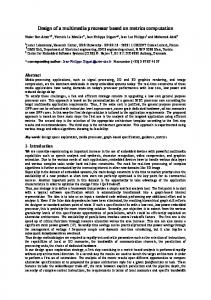
Fig. 2. Simulation results and union bound (UB) of the systematic optimal rate 2/3 and 2/4 codes. IV.1.2. Rate 3/n Systematic Code Search For the rates 3/4 up to 3/7 we can apply a reduced search similar to what was used for the rate 2/4 code. That is we are forcing the parity parts of the codewords that correspond to complementary systematic parts to be the same, and thus we make sure those codeword pairs have minimum |ρ|. The systematic codes found for rates 3/4 up to 3/7 are given below:
37
• Rate 3/4:
∗ C3/4
=
0 0 0 0 0 0 1 0 0 1 0 0 0 1 1 0 1 0 0 0 1 0 1 0 1 1 0 0
,
(4.5)
1 1 1 0 Sρ∗ = {(0, 12), (2/4, 16)}.
• Rate 3/5:
∗ C3/5
=
0 0 0 0 0 0 0 1 0 0 0 1 0 0 1 0 1 1 0 1 1 0 0 0 1 1 0 1 0 1 1 1 0 0 0 1 1 1 0 0
Sρ∗ = {(1/5, 24), (3/5, 4)}.
,
(4.6)
38
• Rate 3/6:
∗ C3/6
=
0 0 0 0 0 0 0 0 1 0 0 1 0 1 0 0 1 0 0 1 1 0 1 1 1 0 0 0 1 1 1 0 1 0 1 0 1 1 0 0 0 1
,
(4.7)
1 1 1 0 0 0 Sρ∗ = {(0, 16), (1/3, 12)}.
• Rate 3/7:
∗ C3/7
=
0 0 0 0 0 0 0 0 0 1 0 0 1 1 0 1 0 0 1 0 1 0 1 1 0 1 1 0 1 0 0 0 1 1 0 1 0 1 0 1 0 1 1 1 0 0 0 1 1 1 1 1 0 0 0 0
Sρ∗ = {(1/7, 28)}.
,
(4.8)
39
• Rate 3/8: For the rate 3/8 code search, we are similarly forcing the first 4 bits of the parity parts of the codewords that correspond to complementary systematic parts to be the same, while setting the remaining bit to be complementary. For example consider two such codewords of the rate 3/8 systematic code: d1 = [0, 0, 0, b0 , b1 , b2 , b3 , b4 ]T , and d2 = [1, 1, 1, b5 , b6 , b7 , b8 , b9 ]T .
If we set
[b5 , b6 , b7 , b8 , b9 ] = [b0 , b1 , b2 , b3 , b4 ], we make sure that this codeword pair has the minimum possible |ρ| = 0. Therefore we reduced the search from 240 to 220 codes. The result of this search is the following orthogonal systematic code (equals to a Hadamard code, H8 , with interchanged columns):
∗ C3/8
=
0 0 0 0 0 0 0 0 0 0 1 0 0 1 1 1 0 1 0 0 1 0 1 1 0 1 1 0 1 1 0 0 1 0 0 0 1 1 0 1 1 0 1 0 1 0 1 0 1 1 0 0 0 1 1 0
,
(4.9)
1 1 1 0 0 0 0 1 Sρ∗ = {(0, 28)}.
By simple observation the rate 3/7 and 3/8 codes are optimal since they have optimal ρ-spectra. From [43] the rate 3/6 code is also optimal. For the rate 3/4 code we run a full search (over 232 codes) and verified that this code has optimal spectrum, and we also verified the optimality of the rate 3/5 code (over the systematic codes though)
40
by running a full search over the parity part. For the performance (union bound, Eq. (3.8) ) of the aforementioned codes, indicatively we give that 10−2 WER is achieved ∗ ∗ code at SNRb = 24.42dB. for the C3/8 code at SNRb = 23.67dB, while for the C3/4
From the resulting optimal codes, we observe that:
∗ ∗ ∗ C2/4 = [C2/3 , c0 ], c0 the fourth column of C2/4 ,
(4.10)
and
∗ ∗ ∗ C3/5 = [C3/4 , c1 ], c1 the fifth column of C3/5 , ∗ ∗ ∗ C3/6 = [C3/5 , c2 ], c2 the sixth column of C3/6 ,
(4.11)
∗ ∗ ∗ C3/7 = [C3/6 , c3 ], c3 the seventh column of C3/7 , ∗ ∗ ∗ C3/8 = [C3/7 , c4 ], c4 the eighth column of C3/8 .
This observation, suggests a nested search, similar to the nested convolutional code search in [52], where a lower rate code is obtained by adding the best code column to a higher rate code. IV.1.3. Nested Search Assume we are given a (ξ, k) binary block code Ck/ξ (i.e. of rate k/n), and want to find the best possible (n, k) code (n > ξ) using a nested search. The steps of the nested search are summarized below: 1. Set j = ξ + 1. 2. Search over the possible (j, k) block codes Ck/j = [Ck/(j−1) , c], where c is an M -bit vector to be found from a search, to yield the best code C 0 k/j , having
41
optimal spectrum over all the spectra of the search. 3. Set Ck/j = C 0 k/j . 4. Set j = j + 1. 5. If j > n Stop, else go to Step 2.
Step 2 of the nested search can be done in a number of ways, depending mostly on k. The following search methods, for example, have been used in Step 2, classified in the order of the complexity of the nested search required to find a systematic rate k/n code, starting from the rate k/k systematic code (complexity is given in terms of the number of codes searched, irrelevant of their length n ≤ M , M = 2k ):
1. Full search. The complexity is
Φ = (n − k) × 2M .
(4.12)
2. Reduced search. For codes with n ≤ 2k+1, we force the parity bits corresponding to complementary systematic parts to be equal, and for codes with n > 2k + 1 we alternatively set those parity bits to be complementary for n even, and equal for n odd (cf. §IV.1.1 and §IV.1.2). Therefore we achieve for these codeword pairs the minimum possible |ρ|. The complexity using this method is
Φ = (n − k) × 2M/2 .
(4.13)
Using similar arguments, based on the structure of the k/k systematic code,
42
one can reduce the complexity to Φ ∝ 2M/4 , and so on (see Appendix D).
3. Hyper-reduced search (see Appendix D). In this method, we let the c vector take only columns of the HM Hadamard code (3.24). We observed that the systematic part of the code is simply the M/2, M/4, . . . , 2, 1st columns of the HM (counting starts from 0), cf. Appendix B. Therefore we find the first code of rate
k k+1
by searching over M − k columns of the HM (excluding the k
systematic columns), the code of rate
k k+2
by searching over M − k − 1 columns
of HM , and so on (code Ck/j must have different columns ∀j). The complexity of the nested search using this method is only
Φ=
M −k X
j ≤ (n − k)(M − k).
(4.14)
j=M −n+1
¤ All these search methods2 yield at the end, i.e. for code rates k/(M − 1) and ¡ ¢ ¡ ¢ k/M , optimal codes. That is they have ρ-spectra equal to ( M1−1 , M2 ) and (0, M2 ) respectively. One can easily verify that if we take any M − 1 columns of HM to form a rate k/(M − 1) code, this code is optimal. In this category also belongs the reduced (7,4,3) Hamming code which appeared in [35]. See also related work in [53]. Furthermore all search methods found to yield equivalent codes (same ρ-spectrum), for those ranges of k that agree. Two exceptions were the rate 4/10 and 5/18 codes found with method 2, which have higher ρmax than the other methods. Note that the codes derived from Method 3 are linear since they consist of columns of the linear HM Hadamard code. 2
Method 1 was used for k ≤ 4, method 2 for k ≤ 5, and method 3 for k ≤ 9. Above these values complexity is a problem (for the current computer power).
43
For an (n, k) linear binary block code Ck/n employed on the block fading channel with non-coherent ML detection, the error probability for the transmission of the mth -codeword is the same for all m, [4, p. 439] (in our case the block fading channel is binary-input symmetric). Assuming that the all-zero codeword was transmitted, the probability of a word error is upper bounded by the union-bound [4, p. 440], (3.6),
P (e) ≤
M −1 X
P2 (ρ2m )
(4.15)
m=1
where ρm = 1 − 2wm /n is the normalized cross-correlation of the mth codeword pair (0th codeword, mth codeword ), codeword 0th is the all-zero codeword, and wm is the weight of the mth codeword. Thus the linearity of the block codes derived from Method 3 gives rise to a 4th search method for the Step 2 of the nested search: We use in this search the union bound (4.15), (3.10) to select the best code, which requires (per code) the calculation of only M − 1 weights, thus reducing dramatically the complexity (as compared to calculate the (full) pairwise ρ-spectrum which requires ¡ ¢ calculation of M2 cross-correlations per code). That is, we will select the best code as the one which has the optimal short ρ-spectrum (over the limited search), that results only from the weight calculation (as opposed to all the possible pairs), cf. §III.1. This is Method 4, and the codes found are, as expected, identical to those of Method 3, but with Method 4 we can more easily find codes with k ≥ 10, that we were not able to find (due to complexity) with Method 3. In the dissertation, unless otherwise stated, we assume that method 4 is used in the step 2 of the aforementioned (forward) nested search.
44
a. Best Rate k/(k + 1) Code Method 3 of the nested search indicates that the columns of the HM matrix can be used to find a best code (if not optimal). But so far our nested search was based on (started from) the rate k/k systematic code, which as we noted, is comprising from HM ’s columns (Appendix B). So here, we will search for the best rate k/(k + 1) codes, whose k + 1 columns are simply some columns of the HM matrix, in order to see whether the use of the systematic k/k code for the beginning of the nested search is a good choice or not. ¡M¢ The complexity of finding such codes is k+1 . We searched for codes, up to k = 5, and found them having identical ρ-spectrum with the systematic k/(k + 1) codes found with method 3. ¡¢ More specifically for k = 3, there were 69 (out of 84 = 70) codes with optimal ρ-spectrum, for k = 4 there were 4353 (out of 4368), and for k = 5 there were 444416 (out of 906192) best 3 codes. Therefore we see that (at least for k ≤ 5) the systematic k/k code is an optimal (or best) choice to start the nested search. However for all k the systematic code is a good choice to start the nested search, since for the rate k/(k + 1) code the nested search will pick at least a min-ρmax code, e.g. the systematic pilot rate k/(k + 1) code, cf. §III.3.1. We verified also for a few code rates that starting our nested search (Methods 3, 4) with just the first column of the HM matrix (i.e. the all-zero column), codes with identical ρ-spectrum were obtained as if we were started with the rate k/k systematic code (see also §VI.1.1, [43]). 3
Here (k = 4, 5) best means the best code found over the corresponding search. For k = 3 though, we had verified by full search the optimality of the corresponding ρ-spectrum.
45
IV.1.4. Backward Nested Search The aforementioned nested search proceeds forward. Likewise, we can have a backward nested search where we begin from a Ck/M code (e.g. the HM code, M = 2k ), and in each iteration we remove an appropriate column until we get to the desired Ck/n code (n < M ). Similar to the (forward) nested search, the backward nested search steps are as follows:
1. Set j = M − 1. 2. Search over the possible (j, k) block codes Ck/j = Ck/(j+1) \{c}, where c a column of Ck/(j+1) , to yield the best code C 0 k/j , having the optimal ρ-spectrum over all the yielded spectra of the search. 3. Set Ck/j = C 0 k/j . 4. Set j = j − 1. 5. If j < n Stop, else go to Step 2. IV.1.5. Enhanced Nested Search Because of the low complexity of the nested search, we could possibly find better codes if in each iteration we were seeking for two or more columns concurrently. For example, if were looking for two columns the enhanced nested search will be as follows, assuming we are given a (ξ, k) block code Ck/ξ : 1. Set j = ξ + 2.
46
2. Search over the possible (j, k) block codes Ck/j = [Ck/(j−2) , c1 , c2 ], where c1 , c2 are M -bit vectors to be found from a search, to yield the best code C 0 k/j , having optimal spectrum over all the spectra of the search. 3. Set Ck/j = C 0 k/j . 4. Set j = j + 2. 5. If j > n (for some n) Stop, else go to Step 2.
All the search methods for Step 2 mentioned for the forward nested search may be applied here also. In the results shown later, we assume only search over 2 columns with use of Method 4. Note that the forward nested search can be combined with the enhanced nested search. For example in the aforementioned example if ξ = 5, we will find with the enhanced nested search codes with n = 7, 9, 11, . . .. In that case, we can find a code with n = 6 using the nested search, and then switch to the enhanced nested search to find codes with n = 8, 10, 12, . . .. Similarly also to the enhanced nested search, we can have an enhanced backward nested search. IV.2. Generalized Nested Search Methods In the following we will summarize and generalize the previously derived, for the binary codes over the noncoherent fading channel, nested search methods. In these nested search methods we search over the columns of a CM,M unitary code4 (see §III.4.2) in a nested way to obtain a best code. The motivation behind 4
For the CM,M codes HM and IM , the search over the code columns is equivalent to the search over the columns of the corresponding generator matrix mT .
47
this was explained in the previous section ([46, 49]) and, in short, it is based on the observation (for some cases) that HM , IM , SM codes achieve the bounds on dmin , as well as on maximum |ρ| (ρmax ). Three basic forms of nested search are again considered, that is forward, backward and enhanced. IV.2.1. Generalized Forward Nested Search The forward nested search steps, assuming we are given a block code CM,ξ and want to find the best CM,n code (n > ξ), are summarized below:
1. Set j = ξ + 1. 2. Search over the possible CM,j block codes CM,j = [CM,j−1 , c], where c is a column of a CM,M code, to yield the best code C 0 M,j , having optimal metric spectrum over all the metric spectra of the search. 3. Set CM,j = C 0 M,j . 4. Set j = j + 1. 5. If j > n Stop, else go to Step 2.
The forward nested search can typically start with the systematic CM,k code [46], provided the CM,M code has the systematic columns, or even the CM,1 code [49], which is a single column, e.g. one column of a CM,M code (chosen randomly, or through some heuristic limited search). However if complexity permits, we can start, for example, with the CM,ξ block code resulting from the full search over-the-columns of the CM,M code (we will cover this in §IV.3.1).
48
We have also chosen to place the restriction that a code must have distinct columns, so that for n = M we will get a unitary CM,M code, e.g. HM , IM , SM . It must be mentioned that in Step 2 of the nested search, there may be more than one c vectors that yield best codes, i.e. codes having the optimal metric spectrum over the spectra of the limited search of the Step 2. In this dissertation, in order to cut down the complexity, we select the first c vector found to yield the best code. However from simulations we found that by relaxing this restriction better codes may be found (due to the nested nature of the search). IV.2.2. Generalized Backward Nested Search In the backward nested search we start from a unitary CM,M code, and iteratively we end up to the best CM,n code (n < M ), by removing an appropriate column in each iteration. Similar to the forward nested search of the previous subsection, the generalized backward nested search steps are as follows: 1. Set j = M − 1. 2. Search over the possible CM,j block codes CM,j = CM,j+1 \ {c}, where c is a column of CM,j+1 , to yield the best code C 0 M,j , having optimal metric spectrum over all the metric spectra of the search. 3. Set CM,j = C 0 M,j . 4. Set j = j − 1. 5. If j < n Stop, else go to Step 2.
49
IV.2.3. Generalized Enhanced Forward/Backward Nested Search Again, due to the low complexity of the aforementioned generalized nested search methods, it is likely that we can find better codes if in each iteration we were seeking for two or more columns concurrently. For example, if we were looking for two columns, the enhanced forward nested search will be as follows, assuming we are given a block code CM,ξ :
1. Set j = ξ + 2. 2. Search over the possible CM,j block codes CM,j = [CM,j−2 , c1 , c2 ], where c1 , c2 are columns of a CM,M code, to yield the best code C 0 M,j having optimal metric spectrum over all the metric spectra of the search. 3. Set CM,j = C 0 M,j . 4. Set j = j + 2. 5. If j > n (for some n) Stop, else go to Step 2.
Note that the generalized forward nested search can be combined with the generalized enhanced forward nested search, similar to §IV.1.5. Again, similarly also to the Enhanced Forward Nested Search we can have an Enhanced Backward Nested Search. The derivation is straightforward, and hence omitted.
So far, we concentrated on CM,n block codes with n ≤ M . For n > M we can proceed as with the previous methodology. That is we can “concatenate” α CM,M codes (α > 1), to form a code of size M × αM and perform the aforementioned search methods over the columns of this big code, instead of the single CM,M code.
50
IV.3. Other Common Search Methods Besides the aforementioned proposed nested search methodology, we will perform also for comparison various typical searches, based on exhaustive and random search approaches. IV.3.1. Full (Exhaustive) Search In the full, otherwise exhausted, search we recognize various types. For example, there is the full search over all the elements of the code, say CM,n code with elements from a Q-ary alphabet. This search is highly complex since it requires a search over QM ×n codes. If on the other hand we constrain the columns of the code to be unique columns ¡ ¢ of a unitary matrix, say CM,M of §III.4.2, then the full search is over M codes n (full over-the-columns of the CM,M code, search), and it is independent of the code’s alphabet Q. IV.3.2. Random Search Although the codes of the nested search methods can be obtained with low computational complexity, they depend on the codes of the previous iteration, which has as a consequence that many good codes may not be obtained. On the other hand, the full search has tremendous complexity, e.g. the optimal ¡ ¢ selection of n out of M Hadamard columns requires a search over M codes, which n ¡1024¢ maybe impractical for large M (e.g. 512 ≈ 10306 ). Therefore, in these cases, it is also common to perform a random search to deal with the high search complexity. Similarly to the various cases of “full search”, we recognize also various random search approaches. That is a random search over all
51
the elements of the code, or random search over unique columns of e.g. a unitary matrix (see also [34, 3]). However, a random search may have a negligible probability to find a good code if the corresponding full search size is large, but due to its adjustable complexity (which depends on the run-time) we adopted it to try to find better codes, if possible, to that of the nested search. In more detail, the implementation of the random column search in this dissertation, is as follows: To find a CM,n code, we run a search over Λ codes (for some Λ), where each of these Λ codes is a random selection of n distinct columns of a CM,M unitary matrix. Since the selection is random, there is a probability that the ¡ ¢ same code appears in the search more than once (for large M compared to Λ, this n probability is small), and there is no effort to avoid that for complexity reasons. The random number generator used was the “Mersenne-Twister” [54, 55]. IV.4. Indicative Complexity Comparison of the Nested Search Method At this point, it is useful to present a complexity comparison between search methods for binary block codes for the noncoherent block fading channel. As it will be shown later, our codes for example for the noncoherent fading channel, are either meeting the quantized lower bound on ρmax , cf. §III.3.1, or they are close to it. Therefore, in order to evaluate our nested search, we give a complexity comparison (in the number of codes to be searched) between the full-search and our forward nested search with Method 4 (§IV.1.3), shown in Figure 3. The search complexity gap between the two methods is more than obvious. For example also a rate 11/13 code requires a full search over ∼ 108015 codes, and a nested search over only 4073 codes, while a rate 11/1792 code requires a full
52
search over ∼ 101,104,785 codes, and a nested search over only 2, 042, 807 codes. Additionally, if we take into account that the full search needs a pairwise ρspectrum calculation per code, while the forward nested search with Method 4 calculation of only M − 1 weights per code, the complexity gap increases even further.
53
5
10
4
Complexity in exponents of 10
10
M=256 M=128 M=64 M=32 M=16
3
10
2
10
1
10
0
10
0
50
100
150 n
200
250
300
(a) M = 16, 32, 64, 128, 256. 7
10
6
10
M=4096 M=2048 M=1024 M=512
5
Complexity in exponents of 10
10
4
10
3
10
2
10
1
10
0
10
0
500
1000
1500
2000
2500
3000
3500
4000
4500
n
(b) M = 512, 1024, 2048, 4096. Fig. 3. Full search (upper set of curves) vs. forward nested search (lower set of curves) complexity comparison, in number of codes required to be searched; the lower curve in a set corresponds to the lower corresponding M shown in the legends.
54
CHAPTER V
NEW BLOCK CODES∗ In this chapter we give codes resulting from the search methods of the previous chapter. We will follow, however, a different order and we will present first the codes for the noncoherent block fading channel, for “historic” reasons, since they were developed first [46]. The evaluation of the codes found is performed through comparison of their achieved extremum metric to a metric bound, as those presented in §III.3, as well as to comparison to codes of prior work when feasible. V.1. Noncoherent Block Fading Channel V.1.1. Binary Codes In Figure 4 we have plotted the lower bounds on ρmax , along with the ρmax of the codes resulting from the forward (§IV.1.3) and the backward nested searches (§IV.1.4) for M = 16 and M = 32, based on the HM (3.24). Moreover, for the sake of clarity, we give in Tables II-III the corresponding columns of the Hadamard matrix HM , comprising the codes of Fig. 4(a) found with the forward and backward nested searches. We observe that although these codes have the same ρmax , they are not ∗
c °2004 IEEE. Part of this chapter is reprinted, with permission, from “Block Code Design based on Metric-Spectrum”, by Panayiotis D. Papadimitriou and Costas N. Georghiades, in Proceedings of the IEEE Global Communications Conference (GLOBECOM), Nov. 29 - Dec. 3, 2004, Dallas, TX, USA., from “New linear binary block codes for the AWGN channel”, by Panayiotis D. Papadimitriou and Costas N. Georghiades, in Proceedings of the 38th Asilomar Conference on Signals, Systems and Computers, November 7-10, Pacific Grove, CA, 2004., and from “On Binary Code Design for the Non-Coherent Block Fading Channel”, by Panayiotis D. Papadimitriou and Costas N. Georghiades, in Proceedings of the IEEE Global Communications Conference (GLOBECOM), December 1-5, 2003, San Francisco, CA, USA.
55
Table II. Columns of HM comprising the forward nested search codes of Fig. 4(a). n
5
columns
8,4,2,1,0
6
7
8
15 3
9
10
5 10 12
11 12
13 14
15 16
6
9
13 14
7
11
Table III. Columns of HM comprising the backward nested search codes of Fig. 4(a). n
5
columns
0,15,14,13,11
6
7
8
7 10 9
9 10
11 12 13
14 15
16
6
12
3
1
5
8
4
2
identical. We run also the random column search (based on the HM ) for Λ = 105 codes, cf. §IV.3.2, but it didn’t yield better codes for the corresponding cases. It must be noted that all the codes of this subsection are based on search over the columns of HM (and therefore they are linear codes), unless otherwise stated. Moreover, the codes found with the forward nested search (§IV.1.3) are systematic since the search starts from the systematic rate k/k code (M = 2k ). Figure 5 displays the codes for M = 64 along with the lower bounds. The legend “Search methods” reflects the best of the codes obtained from the forward nested, backward nested, enhanced nested (§IV.1.3 - §IV.1.5) and random column search methods of Chapter IV. Specifically the enhanced nested search for M = 64 yielded better codes (than the other methods) for n = 29, 32, 35, 36, 49, 52, and the random column search for n = 17, 47, 48 (with Λ ≥ 105 ). In Figures 6-7 we have plotted again the ρmax of the best of the codes obtained through the (forward) nested, enhanced nested and backward nested search methods, but for M = 128 and M = 256 correspondingly (denoted in the figure legends as “Search methods”). The random column search with Λ = 105 didn’t yield better codes in these cases.
56
1 Forward Nested Search (method 4) Backward Nested Search Levenshtein’s LB Quantized Levenshtein’s LB
0.9
0.8
0.7
ρmax
0.6
0.5
0.4
0.3
0.2
0.1
0
5
6
7
8
9
10
11
12
13
14
15
16
n
(a) M = 16 (rate 4/n codes). 1 Forward Nested Search (method 4) Backward Nested Search Levenshtein’s LB Quantized Levenshtein’s LB
0.9
0.8
0.7
ρmax
0.6
0.5
0.4
0.3
0.2
0.1
0
6
8
10
12
14
16
18
20
22
24
26
28
30
32
n
(b) M = 32 (rate 5/n codes). Fig. 4. ρmax of our binary codes (based on the HM ) vs. Levenshtein’s lower bound.
ρmax
8
10 12 14 16 18 20 22 24 26 28 30 32 34 36 38 40 42 44 46 48 50 52 54 56 58 60 62 64 n
Search methods Levenshtein’s LB Quantized Levenshtein’s LB
Fig. 5. M = 64 (rate 6/n codes); ρmax of our binary codes (based on the H64 ) vs. Levenshtein’s lower bound.
0
0.1
0.2
0.3
0.4
0.5
0.6
0.7
0.8
0.9
1
57
ρmax
8
16
24
32
40
48
56
64 n
72
80
88
96
104
112
120
Search methods Levenshtein’s LB Quantized Levenshtein’s LB
Fig. 6. M = 128 (rate 7/n codes); ρmax of our binary codes (based on the H128 ) vs. Levenshtein’s lower bound.
0
0.1
0.2
0.3
0.4
0.5
0.6
0.7
0.8
0.9
1
128
58
0
0.1
0.2
0.3
0.4
0.5
0.6
0.7
0.8
0.9
16
32
48
64
80
96
112
128 n
144
160
176
192
208
224
240
Search methods Levenshtein’s LB Quantized Levenshtein’s LB
256
bound.
Fig. 7. M = 256 (rate 8/n codes), n = 9, . . . , 256; ρmax of our binary codes (based on the H256 ) vs. Levenshtein’s lower
ρmax
1
59
60
Figures 8-121 contain the ρmax of the codes found with the forward nested search alone to show its efficiency. The comparison is done with respect to Levenshtein’s lower bounds. For clarity, we have also plotted in Figure 13 the M = 8192 case, cf. Fig. 12, for n = 14, . . . , 64. In Appendix E, we give the listings of all the codes found in this subsection with the forward nested search for k = 4 up to k = 11. For k = 4 they are also given, as previously mentioned, in Table II. Note that the codes of the forward nested search presented in this subsection (i.e. with k = 4 up to k = 13) contain a pilot bit, since they contain the first column (index 0) of the HM (3.24) in their (k + 1)st column. So far, our codes were based on the HM matrix, given in (3.24). In Figure 14 we depict codes found through the (forward) nested search of §IV.1.3 (method 3) with the following differences. The nested search starts from the first column of a Hadamard code, and the columns of the resulted codes are selected (through the search) from the HM matrix (legend “Sylvester”), and from the non-linear Hadamard code obtained from the first Paley construction [56, 57] (legend “first Paley type”). As we observe in Figure 14, the codes based on the HM matrix have in general lower ρmax than the non-linear Hadamard code from the first Paley construction. This result suggests another research direction, that of finding good orthogonal codes, e.g. [56], for our nested search methods. From the presented results in this subsection, we see that our codes exhibit ρmax close to or on the lower bounds. Note also that although some lower rate codes, say k/(n + µ), µ > 0, may have higher ρmax than the k/n code (for some k, n and µ), it 1
For reference purposes we mention that all the rate k/n codes, k + 1 ≤ n ≤ 2k , of the (forward) nested search for k = 10 and k = 13, were obtained using a PC Pentiumr 4 at 2.26GHz, in 22 seconds, and less than 6 hours respectively.
0
0.1
0.2
0.3
0.4
0.5
0.6
0.7
0.8
0.9
32
64
96
128
160
192
224
256 n
288
320
352
384
416
448
480
Forward Nested Search (method 4) Levenshtein’s LB Quantized Levenshtein’s LB
512
Fig. 8. M = 512 (rate 9/n codes), n = 10, . . . , 512; ρmax of our binary codes (based on the H512 ) vs. Levenshtein’s lower bound.
ρmax
1
61
0
0.1
0.2
0.3
0.4
0.5
0.6
0.7
0.8
0.9
64
128
192
256
320
384
448
512 n
576
640
704
768
832
896
960
1024
Forward Nested Search (method 4) Levenshtein’s LB Quantized Levenshtein’s LB
lower bound.
Fig. 9. M = 1024 (rate 10/n codes), n = 11, . . . , 1024; ρmax of our binary codes (based on the H1024 ) vs. Levenshtein’s
ρmax
1
62
0
0.1
0.2
0.3
0.4
0.5
0.6
0.7
0.8
0.9
128
256
384
512
640
768
896
1024 n
1152
1280
1408
1536
1664
1792
1920
2048
Forward Nested Search (method 4) Levenshtein’s LB Quantized Levenshtein’s LB
lower bound.
Fig. 10. M = 2048 (rate 11/n codes), n = 12, . . . , 2048; ρmax of our binary codes (based on the H2048 ) vs. Levenshtein’s
ρmax
1
63
0
0.1
0.2
0.3
0.4
0.5
0.6
0.7
0.8
0.9
256
512
768
1024
1280
1536
1792
2048 n
2304
2560
2816
3072
3328
3584
3840
4096
Forward Nested Search (method 4) Levenshtein’s LB Quantized Levenshtein’s LB
lower bound.
Fig. 11. M = 4096 (rate 12/n codes), n = 13, . . . , 4096; ρmax of our binary codes (based on the H4096 ) vs. Levenshtein’s
ρmax
1
64
0
0.1
0.2
0.3
0.4
0.5
0.6
0.7
0.8
0.9
512
1024
1536
2048
2560
3072
3584
4096 n
4608
5120
5632
6144
6656
7168
7680
8192
Forward Nested Search (method 4) Levenshtein’s LB Quantized Levenshtein’s LB
lower bound.
Fig. 12. M = 8192 (rate 13/n codes), n = 14, . . . , 8192; ρmax of our binary codes (based on the H8192 ) vs. Levenshtein’s
ρmax
1
65
66
0.9 Forward Nested Search (method 4) Levenshtein’s LB Quantized Levenshtein’s LB 0.8
0.7
ρmax
0.6
0.5
0.4
0.3
0.2
0.1
16
20
24
28
32
36
40
44
48
52
56
60
64
n
Fig. 13. M = 8192 (rate 13/n codes), n = 14, . . . , 64; ρmax of our binary codes (based on the H8192 ) vs. Levenshtein’s lower bound. doesn’t mean that they will necessarily perform worse since the multiplicity Nρmax is also important, cf. (3.8), (3.10). Notice that we also list very low rate codes, which may not be practical for use in the fading channel (due to the large bandwidth expansion), but can be used in other channels. For example, one can use the codes designed here for any system requiring sequences with low pairwise cross-correlations, e.g. in a synchronous CDMA system one can replace the Hadamard-Walsh codes with the designed codes to increase system capacity [43] (see also Chapter VI). To the best of our knowledge, this is the first time a large multitude of binary block codes was designed for the noncoherent block fading channel and reported in
67
1 Hadamard (Sylvester) Hadamard (first Paley type) Levenshtein’s LB Quantized Levenshtein’s LB
0.9
0.8
0.7
ρ
max
0.6
0.5
0.4
0.3
0.2
0.1
0
6
8
10
12
14
16
18
20
22
24
26
28
30
32
n
Fig. 14. M = 32 (rate 5/n codes), n = 6, . . . , 32; ρmax of our binary codes (based on H32 (“Sylvester”) and first Paley type Hadamard matrices) vs. Levenshtein’s lower bound. the literature (at least in the form of Figures), for low as well as high code rates. In addition, it seems that reports of actual binary code designs are not present in the literature (to perform a direct comparison with our binary codes) except one found in [35] (see comments in §IV.1.3), with limited however code reports. Binary codes, targeted though for the multiple-access channel (having the ρmax metric as well for design criterion), are reported in [53], but we will refer to them in the appropriate Chapter (Chapter VI). In [32, 3] the authors designed M -PSK block codes based in general on random search (or exhaustive when applicable). However, for the binary case M = 2 there
68
were no codes reported. In [33] the authors introduced an analytical M -PSK linear block code design approach for noncoherent detection, but they were constrained to codes with very small redundancy and didn’t report on any binary codes, i.e. M = 2. V.1.2. Complex Codes In this subsection we present some complex code results of the search methods described in §IV.2, as well as in §IV.3. To simplify here further the search (in terms of computing effort) we paid attention only in the last spectrum line (ρmax , Nδ ), i.e. λ = δ (see definition of the optimal ρ-spectrum). By this, we mean that the selection of the corresponding code is done not with the optimal metric spectrum criterion, but rather with the “best” last spectrum line (which is (ρmax , Nρmax )) criterion (unless otherwise specified). Therefore (in Step 2 when we use nested search) we select the code that either its ρmax is the lowest possible over the search, or if there are multiple codes with same minimal ρmax , then its Nρmax is the lowest possible (if again there is a tie, we select the first found code). In order to get a complex code CM,n (of cardinality M and length n < M ) with small ρmax , we perform in the straightforward approach a full search over the M columns of the CM,M code (3.26), (3.27) and we select those n columns that yield the CM,n code with the best last spectrum line (ρmax , Nδ ). Note that this search requires ¡ ¢ calculation of M cross-correlation spectra, which may be prohibitively complex for n large M , in which case we will switch to the nested search of §IV.2. In Figure 15 we present the ρmax of the CM,n Qary-PSK codes found with the full search over-the-columns for M = 16 (§IV.3.1), where we used the CM,M = SM Unitary matrix (3.27), and in Figure 16 we have the codes found with the same search but using the CM,M = IM Unitary matrix (3.25). Notice that we have included also (Fig. 15) the case Q = 2 which corresponds to binary codes, since in general the
69
1 Q=2 Q=4 Q=8 Q=16 Levenshtein bound
0.9
0.8
0.7
ρmax
0.6
0.5
0.4
0.3
0.2
0.1
0
2
4
6
8
10
12
14
16
n
Fig. 15. ρmax of Qary-PSK codes found with the full over-the-columns search vs. lower bound (based on the S16 unitary matrix); M = 16, 2 ≤ n ≤ M . search details of this subsection are different to those of §V.1.1, hence different codes may be found. In Figure 17 we present the ρmax of the CM,n Qary-PSK codes found for M = 32, with the full search over-the-columns but using the short ρ-spectrum, cf. §III.1 (where again we used the CM,M = SM Unitary matrix (3.27)). Recall that the short ρspectrum, as opposed to the (full) ρ-spectrum, contains not all the pairwise absolute crosscorrelations, but rather all the pairwise absolute crosscorrelations with respect to a specific codeword. Therefore the search using the short ρ-spectrum is much less complex than if we were using the (full) ρ-spectrum, since it requires only M − 1 cross-correlations. This complexity reduction can make our search methods feasible
70
1 Q=4 Levenshtein bound 0.9
0.8
0.7
ρmax
0.6
0.5
0.4
0.3
0.2
0.1
0
2
4
6
8
10
12
14
16
n
Fig. 16. ρmax of Qary-PSK codes found with the full over-the-columns search vs. lower bound (based on the I16 unitary matrix); M = 16, 2 ≤ n ≤ M . for getting codes with larger cardinality and codeword length. It can be shown [34, 3], that if from DM (3.26) we pick any n columns, the resulting CM,n code has absolute pairwise cross-correlations:
|ρij | = f (|i − j|)
(5.1)
which are a function of the corresponding absolute rows difference; here i, j are the indices of two rows (codewords) of CM,n . Therefore, since the pairwise crosscorrelations have the form of (5.1), instead of calculating the whole pairwise cross¡ ¢ correlation spectrum of M2 pairwise cross-correlations (full ρ-spectrum), it suffices
71
to calculate only M − 1 pairwise cross-correlations, i.e. ρ0j , j = 1, 2, . . . , M − 1 (short ρ-spectrum). However, it can be shown that (5.1) is not valid in general, if the CM,n code is resulting from the DQ according to (3.27) or (3.28), i.e. for Q < M . But due to the dramatic complexity reduction we have example results by using the short ρ-spectrum that otherwise would be impossible to obtain. A reasonable question arises here, that of whether the ρmax calculated with the full and the short ρ-spectra respectively are equal. This question will be tackled in the sequel in this subsection in the discussion of the results. If we want now to get codes of higher cardinality and length, we’ll have to switch to the low complexity nested search methods. In the forward nested search, we use the CM,M = SM Unitary matrix (3.27), starting the search from just the first column of the SM , i.e. ξ = 1, cf. (§IV.2.1), unless otherwise stated. In the backward nested search which is also based on SM , and in order to be consistent with the forward nested search, in this subsection, we chose not to remove the first column of the SM code in any iteration of the backward nested search. In Figures 18-19, we have the codes for M = 64 and M = 256 respectively, resulting from the forward nested search, where we observe that for moderate to large n, Qary-PSK codes of small Q achieve ρmax close to that of the larger constellation codes. Note that in the case Q = 256 (in Figure 19) we made use of the short ρ-spectrum. Figure 20 depicts the search results with the forward nested search for the case of M = Q = 1024. Figure 21 contains the comparison between the forward nested and backward nested search for M = Q = 256. As expected, the forward nested search yields in general better codes for small n, and the backward nested search for large n. However the difference in ρmax of the two methods at high n is very small (for the
0
0.1
0.2
0.3
0.4
0.5
0.6
0.7
0.8
0.9
2
4
6
8
10
12
14
16 n
18
20
22
24
26
28
30
Q=2 Q=4 Q=8 Q=16 Q=32 Levenshtein bound
32
the short ρ-spectrum, and are based on the S32 unitary matrix); M = 32, 2 ≤ n ≤ M .
Fig. 17. ρmax of Qary-PSK codes vs. lower bound (the codes were found with the full over-the-columns search but using
ρmax
1
72
ρmax
4
8
12
16
20
24
28
32 n
36
40
44
48
52
56
60
Q=2, forward nested search Q=4, forward nested search Q=8, forward nested search Q=16, forward nested search Q=32, forward nested search Q=64, forward nested search Levenshtein bound
Fig. 18. ρmax of Qary-PSK codes vs. lower bound (based on the S64 unitary matrix); M = 64, 2 ≤ n ≤ M .
0
0.1
0.2
0.3
0.4
0.5
0.6
0.7
0.8
0.9
1
64
73
ρmax
16
32
48
64
80
96
112
128 n
144
160
176
192
208
224
240
Q=4, forward nested search Q=256, forward nested search (short) Levenshtein bound
Fig. 19. ρmax of Qary-PSK codes vs. lower bound (based on the S256 unitary matrix); M = 256, 2 ≤ n ≤ M .
0
0.1
0.2
0.3
0.4
0.5
0.6
0.7
0.8
0.9
1
256
74
75
cases shown). We also observed that when we used the short ρ-spectrum in the code-search of Figures 15, 19 (for Q < M ), codes with identical ρmax were found. Furthermore for the codes of Fig. 17, ρmax calculated via the short ρ-spectrum was equal to that via the (full) ρ-spectrum. More research though needs to be performed towards the relationship between the (full) ρ-spectrum and the short ρ-spectrum (and if their corresponding ρmax are equal in general) for codes designed through (3.27). Lastly, in Figures 22-23 we show the importance on the choice of the unitary matrix to be used in the forward nested search, since it affects the efficiency of the search method. Moreover results with random search over Λ = 105 codes, according to §IV.3.2 are given, showing that when the full search (over the columns of a unitary ¡ ¢ matrix) size M is not very large, random search is capable to give good codes. n In the figures of this subsection, we have also plotted the Levenshtein bound [45] (see also §III.3.2). We see that the Qary-PSK codes have a ρmax close to the lower bound. However the aforementioned bound has been constructed for codes with elements from the complex alphabet and not specifically from the Qary-PSK alphabet, therefore some looseness is to be expected. We believe also that with some more programming effort, i.e. by including more spectral lines in the nested search, better codes may be obtained, at the additional expense of higher complexity search. In the literature (as briefly mentioned in the literature survey of §II.3), there also exists a Fourier-based construction of M -PSK codes [34] by randomly selecting n rows of the DM DFT matrix such that the resulting vectors have as little correlation ¡ ¢ as possible. However this method of [34] is effective as long as M is not very large, n and is limited to Q = M . For Q < M though, we can form a CM,M code according to §III.4.2 and perform
ρmax
64
128
192
256
320
384
448
512 n
576
640
704
768
832
896
960
1024
Q=1024, forward nested search (short) Levenshtein bound
Fig. 20. ρmax of 1024-PSK codes vs. lower bound (based on the S1024 unitary matrix); M = 1024, 2 ≤ n ≤ M .
0
0.1
0.2
0.3
0.4
0.5
0.6
0.7
0.8
0.9
1
76
0
0.1
0.2
0.3
0.4
0.5
0.6
0.7
0.8
0.9
16
32
48
64
80
96
112
128 n
144
160
176
192
208
224
240
Q=256, forward nested search (short) Q=256, backward nested search (short) Levenshtein bound
256
backward nested search; M = 256, 2 ≤ n ≤ M .
Fig. 21. ρmax of 256-PSK codes vs. lower bound (based on the S256 unitary matrix); Comparison of forward nested vs.
ρmax
1
77
0
0.1
0.2
0.3
0.4
0.5
0.6
0.7
0.8
0.9
4
8
12
16
20
24
28
32 n
36
40
44
48
52
56
Levenshtein bound
60
Q=4, S , forward nested search 64 Q=4, I64, forward nested search 5 Q=4, I64, random search (Λ = 10 )
64
Fig. 22. ρmax of Qary-PSK codes vs. lower bound (based on the S64 , and I64 unitary matrices); M = 64, 2 ≤ n ≤ M .
ρmax
1
78
32
48
64
80
96
112
128 n
144
160
176
0
0.1
0.2
0.3
0.4
0.5
0.6
192
208
224
240
0.8
16
Levenshtein bound
0.9
0.7
Q=4, S , forward nested search 256 Q=4, I , forward nested search 256 Q=16, I256, forward nested search 5 Q=4, I256, random search (Λ = 10 )
256
Fig. 23. ρmax of Qary-PSK codes vs. lower bound (based on the S256 , and I256 unitary matrices); M = 256, 2 ≤ n ≤ M .
ρmax
1
79
80
random search, cf. §IV.3.2, Figures 22-23, on the columns of that code to pick those n columns such that the resulting CM,n code is best. Although it is risky to compare versus random search methods, we would say for example (based on simulations), that for Q = M = 256 the aforementioned method of [34] yields the same or lower ρmax codes than our nested search approximately for n up to 20, provided reasonable search time (it was tested for 100 times the corresponding search time required by our nested search). Besides this, there exists an algebraic structure to find complex block codes with low ρmax of cardinality M = QK (for some integer K) and length n, by using Q-PSK modulation on codes from the ring of integers modulo Q, ZQ , [32, 3, 33, 34]. In [34], in order to reduce the complexity of the algebraic approach, the authors performed a random search over systematic generator matrices. If we were to compare their approach to ours in obtaining low ρmax CM,n codes, we would say that it is very good for small n, but very complicated for today’s computer power, for large n. For example a full search to obtain a C256,128 code with say Q = 4 (and the algebraic approach) requires a search over ≈ 10298 codes, which means that a random search (of maybe ≈ 107 codes) may have a small probability to find a good code. For the same parameters, our nested search requires search over only 32640 codes to find all the C256,n codes with 2 ≤ n ≤ 256! We also believe that our methodology gives more design flexibility, e.g. Q-PSK codes of cardinality M cannot be obtained with the algebraic approach, unless K = logQ M is an integer. Lastly the codes derived through the algebraic approach are not guaranteed to be max-SC codes (for more details on these codes, see §VI.2 (6.12)). We performed very long random searches according to the algebraic approach of [34] and the ρmax comparison to our forward nested search codes, cf. Fig. 23, 21, is given in Tables IV, V. Particularly for the codes with length n ≥ 128, we stopped the
81
Table IV. Code ρmax comparison; M = 256, Q = 4. n
16
64
128
192
224
Forward nested
0.39528
0.16087
0.09111 0.05753 0.03993
Random [34]
0.37500
0.18222
0.12932 0.10546 0.10278
Table V. Code ρmax comparison; M = 256, Q = 256. n
16
128
192
Forward nested
0.40103
0.09756 0.05715
Random [34]
0.37665
0.12979 0.10531
random searches after not seeing any change in ρmax for several days. For example also, the total number of codes randomly searched [34] for the code C256,128 (Q = 256) was approximately 1.14 · 107 . V.2. AWGN Channel V.2.1. Binary Codes In this subsection we present code results for the AWGN channel, from the search methods described in §IV.2, where we have used the Hadamard code HM (3.24) as the CM,M code (M = 2k ) required by our search methods. We start the forward nested search with the systematic CM,k code, i.e. ξ = k, cf. §IV.2.1 (therefore all the codes found with this method are systematic). Note that the systematic CM,k block code consists of the M/2, M/4, . . . , 2, 1st columns of the M × M linear binary Hadamard matrix HM (counting starts from 0), see Appendix
82
Forward Nested Search Backward Nested Search Bound
8
7
6
dmin
5
4
3
2
1
0
5
6
7
8
9
10
11
12
13
14
15
16
n
Fig. 24. dmin of linear binary block codes (based on the H16 ) vs. coexisting lower and upper bounds; k = 4, 5 ≤ n ≤ 2k . B. Likewise, in the backward nested search, in order to be consistent with the forward nested search, we don’t remove the aforementioned “systematic” columns (i.e. the columns of the systematic CM,k code). In Figures 24-25 we depict the minimum (Hamming) distance dmin of the codes found through the forward and backward nested searches for k = 4 and k = 5, respectively. It is obvious that the best of the codes of these two search methods are max-dmin codes, since they achieve the coexisting upper and lower bounds on dmin [36]. For example also we give in the following vectors cf and cb , the corresponding columns of the Hadamard matrix H32 (3.24), comprising the codes of Fig. 25 (k = 5)
83
16
Forward Nested Search Backward Nested Search Bound
14
12
dmin
10
8
6
4
2
0
10
15
20
25
30
n
Fig. 25. dmin of linear binary block codes (based on the H32 ) vs. coexisting lower and upper bounds; k = 5, 6 ≤ n ≤ 2k . of the forward and backward nested searches respectively.
n=15
z }| { n=9 z }| { cf = [16, 8, 4, 2, 1, 31, 7, 11, 21, 25, 13, 14, 19, 22, 26, 28, 3, 5, 9, 17, 30, 6, 10, 18, 29, 12, 20, 27, 15, 23, 24, 0], (5.2)
84
32 Forward Nested Search Backward Nested Search Enhanced Forward Nested Search Bound
30 28 26 24 22 20 dmin
18 16 14 12 10 8 6 4 2 0
8
12
16
20
24
28
32
36 n
40
44
48
52
56
60
64
Fig. 26. dmin of linear binary block codes (based on the H64 ) vs. coexisting lower and upper bounds; k = 6, 7 ≤ n ≤ 2k .
n=15
z }| { n=9 z }| { cb = [16, 8, 4, 2, 1, 15, 22, 21, 12, 19, 11, 13, 23, 10, 20, 18, 14, 17, 9, 30, 29, 27, 24, 7, 26, 25, 6, 5, 28, 3, 31, 0]. (5.3) In Figure 26 the codes found with k = 6 are depicted. In more detail, in addition to the forward and backward nested search methods we have plotted the results of the enhanced forward nested search (over 2 columns). We observe that the best of the codes either achieve the dmin bound or they are close to it. Recall that in the nested search methods, the codes depend on the previously
85
64 Search methods Bound
60 56 52 48 44 40
dmin
36 32 28 24 20 16 12 8 4 0
8
16
24
32
40
48
56
64
72
80
88
96
104
112
120
128
n
Fig. 27. dmin of linear binary block codes (based on the H128 ) vs. coexisting lower and upper bounds; k = 7, 8 ≤ n ≤ 2k . found codes. We have found that by ad-hoc modification of the nested search better codes may be found. For example, recall that in the backward nested search we don’t remove the systematic columns during the search. By checking also some cases, we observed that the forward nested search “selects” the last column of the Hadamard matrix for the (k + 1)st column. Therefore by not removing this column from the backward nested search in addition to the systematic columns, we found a few better codes than the other methods. The best of the codes found with this ad-hoc modification, as well the other of our nested search methods are depicted for k = 7 in Figure 27, where again we see that either they meet the dmin bound either they are close to it.
86
In order to show the efficiency of the forward nested search alone, we have plotted in Figure 28 the resulted low dmin codes for k = 14. A PC Pentiumr 4 at 2.26GHz was employed and the execution time of the forward nested search to get all the codes of rates k/(k + 1) to k/2k , for k = 7 and k = 14, was approximately 1 second and 49 hours, respectively. In order to have a comparison with state-of-art codes (besides the comparison we have to the ultimate criterion, i.e. the dmin bound) we chose for example the BCH code (n, k) = (15, 5) with generator polynomial 24678 in octal [4, p. 437] which has dmin = 7. This code has weight multiplicities (distribution) N7 = 15, N8 = 15 and N15 = 1 (N0 = 1). Our best code found with the forward nested search (Fig. 25) has the same dmin = 7 and exactly the same weight distribution. The code is given in (5.2) for n = 15. However there are BCH codes (and even there should be other block codes) that achieve a larger dmin compared to our codes, e.g. the (31, 6) BCH code compared to our codes of Fig. 26, since no optimality of our codes is claimed. We believe that with some more programming effort, along the lines of the enhanced nested search codes of larger dmin may be found. Lastly we would like to demonstrate a very simple construction (named “Direct” construction) of good linear block codes of certain rates without the need for any search. By comparing the dmin bounds [36] and the structure of the linear Hadamard matrices, it can be easily inferred that one may get good codes around the rates of k/2k−1 , k/(2k−1 + 2k−2 ), and so on, by simply using parts of the Hadamard matrices as codes. For example, the codes of rate k/n are constructed from the M −n, . . . , M − 2, M − 1 columns (M = 2k ) of the Hadamard matrix (assuming first column’s index is 0). The dmin of the codes found for k = 6, 7 is given in Figures 29-30 respectively, where we observe many max-dmin codes in the aforementioned code rates.
dmin
0
512
1024
1536
2048
2560
3072
3584
4096
4608
5120
5632
6144
6656
7168
7680
8192
1024
3072
4096
5120
6144
7168
8192 n
9216
10240
11264
12288
13312
14336
Fig. 28. dmin of linear binary block codes (based on the H16384 ); k = 14, 15 ≤ n ≤ 2k .
2048
Forward Nested Search
15360
16384
87
88
32 Direct Construction Bound
30 28 26 24 22 20 dmin
18 16 14 12 10 8 6 4 2 0
8
12
16
20
24
28
32
36 n
40
44
48
52
56
60
64
Fig. 29. dmin of linear binary block codes resulted from the Direct construction vs. coexisting lower and upper bounds; k = 6, 7 ≤ n ≤ 2k . Moreover the (n, k) = (2k−1 −1, k) block codes found with the direct construction for k = 4, 5, 6, 7, 8, 9, have same dmin as the corresponding BCH codes [58], [4, p. 437]. One could also easily get a good code of rate k/(n + αM ), 1 ≤ n ≤ M , α ≥ 1, from a good code of rate k/n by simply concatenating α Hadamard matrices (of size M × M ) to it. The motivation behind it is the observation that the concatenation of Hadamard matrices yield codes with dmin close to or on the dmin bound [36]. From the results in this subsection, we can conclude that good linear binary block codes for the AWGN channel can be designed with our methodology, with small complexity, for a wide range of code rates. Further one may come up with high-rate codes, by using the duals of the ob-
89
64 Direct Construction Bound
60 56 52 48 44 40
dmin
36 32 28 24 20 16 12 8 4 0
8
16
24
32
40
48
56
64
72
80
88
96
104
112
120
128
n
Fig. 30. dmin of linear binary block codes resulted from the Direct construction vs. coexisting lower and upper bounds; k = 7, 8 ≤ n ≤ 2k . tained low-rate codes, for which the weight distribution can be obtained from the corresponding ones of the low-rate codes [11, Ch. 5], [25]. However we will not pursue in this dissertation this research direction. In the literature, there exists a somewhat related to our design methodology construction of linear block codes, based on simplex codes and the notion of anticodes. These codes are constructed from the generator matrix of a binary simplex code (or several copies of it), by deleting certain columns, which form the generator matrix of the anticode. The formation of the anticode now is more involved, using the mathematical tool of projective geometry. The interested reader may consult [11, Ch. 17, §6] and the many references therein.
90
In this subsection we presented a large multitude of linear binary block codes with large dmin (suitable for the AWGN channel), derived from simple searches. Since we already compared the dmin of our codes to the dmin bounds (visually in the figures), which is the ultimate comparison, we won’t proceed to further comparisons with state-of-art codes [1, 11], besides the aforementioned ones. Finally, we would like to comment, based on [51, 59], that although we see that the minimum distance of a code increases in general with increasing n, this doesn’t necessarily translate to better asymptotic performance. The asymptotic performance is better evaluated by the product Rdmin (asymptotic coding gain). This becomes obvious from the following form of the union bound of the probability of codeword error of a linear binary block code over AWGN, cf. (3.10), [4],
P (e) ≤
n X
p Nd Q( 2γb Rd),
(5.4)
d=dmin
where γb is the signal to noise ratio per information bit, R the code rate, dmin is the minimum weight of the code excluding the all-zero codeword, and Nd is the weight multiplicity, which equals the number of times the weight d appears in the code. In Figure 31 we have plotted the contents of Figure 26, where we have as the y-axis the asymptotic coding gain (Rdmin ) instead of dmin . Like in [51], which is for convolutional codes though, we observe that the maximum asymptotic coding gain (bound) is not strictly increasing with n. This means that one may not have to deploy very low rate block codes to achieve a certain asymptotic coding gain.
91
3.5
3
2.5
Rdmin
2 Forward Nested Search Backward Nested Search Enhanced Forward Nested Search Bound
1.5
1
0.5
0
8
12
16
20
24
28
32
36 n
40
44
48
52
56
60
64
Fig. 31. Product Rdmin of linear binary block codes (based on the H64 ) vs. coexisting lower and upper bounds; k = 6, 7 ≤ n ≤ 2k . V.2.2. Complex Codes In this subsection we present complex block codes, minimizing the pairwise squared Euclidean distance, resulting from the search methods of §IV.2 and targeted for the AWGN channel [60]. In more detail, Figure 32 contains complex block codes, minimum d2E (2.13) vs. code length n, of cardinality M = 64. The first three codes of the legend, are based on the CM,M = I64 Unitary matrix, cf. (3.25), with parameters Q = 64 and k = 1. The fourth code is based on the S64 Unitary matrix, cf. (3.27), with Q = 32. It must be noted that in order to reduce the programming effort, in the second steps of the
92
128 Forward Nested Search (Q=64, k=1) Backward Nested Search (Q=64, k=1) Enhanced Forward Nested Search (Q=64, k=1) Forward Nested Search (Q=32) Binary (Lower & Upper) Bound
120 112 104 96 88 80
d2E
72 64 56 48 40 32 24 16 8 0
4
8
12
16
20
24
28
32 n
36
40
44
48
52
56
60
64
Fig. 32. Minimum d2E of complex block codes based on IM and SM , and binary bound vs. code length n; M = 64. nested search methods, we paid attention only to the first spectral line (minimum d2E ), and not to the whole spectrum. In Figure 32 we have also plotted the bound2 on the minimum d2E of binary codes (since the upper-bound of [40] requires M > (Q/3)n , cf. §III.3), which is four times the minimum Hamming distance bound of the codes [36]. We observe that the complex codes are able to offer better performance (increased minimum d2E ) especially at small code lengths; see also Table VI where we have some bandwidth efficient codes that their minimum distance compares favorably with the minimum distance of say 2
The lower and upper bounds are coexisting.
93
Table VI. Some bandwidth efficient codes
2
log2 M n
Type of Search
Unitary Code
M
n
Q
k
mind2E
Random
SM
256
4
32
-
2.39
Random
IM
256
4
256
1
2.69
Random
IM
4096
6
8
4
2.93
Random
IM
4096
6
4096
1
2.95
Full
IM
16
4
16
1
8.00
Random
SM
1024
10
512
-
10.68
-PSK constellation (which has the same bandwidth expansion).
However, we observe some codes with specific length n, which are inferior to the binary bound. For at least these specific lengths n, we can construct good codes using our “Direct” construction method, which is based on our intuition obtained from the structure of Hadamard codes, cf. Fig. 29, [47]. In more detail, the codes of cardinality M and length n are constructed from the M − n, . . . , M − 2, M − 1 columns of an SM Unitary matrix (assuming first column’s index is 0). Codes found with this method are shown in Fig. 33 for Q = 16 and M = 64. To test also the efficiency of the nested search, in Figure 34 we have plot codes found with the forward nested search with M = Q = 10243 . The complex block codes presented achieve in general higher minimum d2E than the bound of binary codes. However the lack of efficient minimum d2E upper-bounds for complex block codes, cf. §III.3, does not let us draw safe conclusion about the difference in the minimum d2E between binary and complex block codes. 3
All the codes from n = 2 to n = 1024 were found in approximately 10 seconds, using a PC with Pentiumr 4 processor at 2.26GHz.
94
128 Direct Construction (Q=16) Binary (Lower & Upper) Bound
120 112 104 96 88 80
d2E
72 64 56 48 40 32 24 16 8 0
4
8
12
16
20
24
28
32 n
36
40
44
48
52
56
60
64
Fig. 33. Minimum d2E of complex block codes found with the Direct Construction, based on S64 , and binary bound vs. code length n; M = 64. 2048 Forward Nested Search (Q=1024, k=1) 1792
1536
d2E
1280
1024
768
512
256
0
128
256
384
512 n
640
768
896
1024
Fig. 34. Minimum d2E of complex block codes found with the forward nested search vs. code length n; M = 1024.
95
V.3. Coherent Fading Channel For the Coherent Fading Channel, we found complex block codes (depicted in Figure 35) through the forward nested search (§IV.2.1), based on the CM,M codes I64 and S64 4 , using the metric B, cf. (3.13), [60], with SNR=10. In more detail, when we use the I64 matrix, we start the nested search with the systematic CM,k code (that is a code containing the k systematic columns of I64 ). On the other hand, when we make use of the S64 matrix in our forward nested search, we start the search with a single column code, containing the 11th column of S64 (chosen simply by a few trials). In both cases however, in order to reduce the search complexity at the Step 2 of the search methods, we paid again attention only in the first spectral line (minimum metric and its corresponding multiplicity), as opposed to the whole metric spectrum. It is observed in Figure 35 that for all codes originated from I64 or S64 , the higher the Q the larger the minimum metric B for the same code length n. Figures 36-37 depict the minimum metrics Ξ and Γ, cf. (3.14), (3.15), of the codes found with the forward nested search, based again on the CM,M codes I64 and S64 . From the comparison of the Figures 35-37 it is evident that the code design for the coherent Rayleigh channel, should look directly on maximizing the minimum B (3.13). If one would try to design codes based independently either on maximizing the minimum Ξ or on maximizing the minimum Γ, although these metrics are independent of the SNR, one may end up with opposite results; for example the codes found with Q = 64 are the best based on metric Ξ, but the worst (in general) based on the 4
When there is no k value in the legend, the corresponding code is based on SM , else on IM .
96
35
10
Q=2, k=6 Q=4, k=3 Q=8, k=2 Q=8 Q=32 Q=64, k=1
30
10
25
10
20
B
10
15
10
10
10
5
10
0
10
0
4
8
12
16
20
24
28
32 n
36
40
44
48
52
56
60
64
Fig. 35. Minimum metric B (SNR=10), cf. (3.13), of linear block codes CM,n , based on I64 and S64 ; M = 64. product distance metric Γ (cf. Figures 36-37). An evaluation of the complex block codes found can not be performed, since we are not aware either of any bounds on the corresponding metrics, neither of any previous complex block codes for the coherent fading channel.
97
35 Q=2, k=6 Q=4, k=3 Q=8, k=2 Q=8 Q=32 Q=64, k=1
30
25
Ξ
20
15
10
5
0
0
4
8
12
16
20
24
28
32 n
36
40
44
48
52
56
60
64
Fig. 36. Minimum metric Ξ, cf. (3.14), of linear block codes CM,n , based on I64 and S64 ; M = 64. V.4. Other Channels with Known Pairwise Error Probability It is obvious that using our code design methodology, best or optimal codes can be found for any transmission channel. The only requirement is the knowledge of the corresponding pairwise error probability or at least an upper-bound of it, out of which we will extract the metric which would be used by our search methods to find the code that optimizes it. There are of course, many other transmission channels of interest, than the ones covered here. However, in order to keep the size of this dissertation reasonable, we won’t present block codes for other channels than the ones already presented in the
98
20
10
Q=2, k=6 Q=4, k=3 Q=8, k=2 Q=8 Q=32 Q=64, k=1
15
Γ, Product Distance
10
10
10
5
10
0
10
0
4
8
12
16
20
24
28
32 n
36
40
44
48
52
56
60
64
Fig. 37. Minimum metric Γ, cf. (3.15), of linear block codes CM,n , based on I64 and S64 ; M = 64. previous sections.
99
CHAPTER VI
APPLICATIONS TO MULTIPLE-ACCESS∗ Besides the application of the designed block codes for their target channel, other applications can be found for communication situations that the same metric dominates the probability of error. In this chapter we will investigate the application of the previously designed codes in the multiple-access communications [4], as well we will propose - when necessary - minor modifications to better match each specific case. VI.1. Binary Code Search Maximizing Total Squared Correlation In [61] it was shown that the sum capacity of the synchronous code division multiple access (CDMA) channel with equal average input energy constraints is maximized with signature (multi-) sets meeting Welch’s lower bound on the total square correlation (TSC)1 . Specifically for binary signature sets, it has been shown [53] that the sum capacity is maximized for optimum TSC signature sets (sets achieving the lower bound on TSC) of certain cardinality and length [62] (see also [61, 63]), while the ∗
c °2004 IEEE. Part of this chapter is reprinted, with permission, from “On a Unified View of Synchronous Multiple-Access Channels: A Bandwidth Efficiency Perspective”, by Panayiotis D. Papadimitriou and Costas N. Georghiades, in Proceedings of the IEEE Wireless Communications and Networking Conference (WCNC), March 21-25, 2004, Atlanta, GA, USA., from “Complex Block Codes with Low CrossCorrelation Spectrum for S-CDMA Systems”, by Panayiotis D. Papadimitriou and Costas N. Georghiades, in Proceedings of the Asilomar Conference on Signals, Systems, and Computers, November 9-12, 2003, Pacific Grove, CA, USA., and from “Code-search for Optimal TSC Binary Sequences with Low Cross-Correlation Spectrum”, by Panayiotis D. Papadimitriou and Costas N. Georghiades, in Proceedings of the Military Communications Conference (MILCOM), October 13-16, 2003, Boston, MA, USA. 1
The so-called Welch’s lower bound on total square correlation (TSC), is a byproduct of Welch’s lower bound on the maximum cross-correlation of a complex set proof [42].
100
rest of the optimum TSC binary signature sets exhibit negligible sum capacity loss as compared to optimum TSC real/complex sequence sets (of the same cardinality and length). On the other hand, optimum TSC sequence sets don’t imply sets with low crosscorrelation spectrum, §IV.1, [46]. If an optimum TSC set [53] has a few pairs with high cross-correlation, this may result in some users experiencing high probability of error since, for example, the latter (assuming for simplicity equal user powers and BPSK modulation) can be upper-bounded by a function of the sum of the pairwise absolute and/or squared cross-correlations of the sequences of the users with respect to the sequence of the user of interest [64, §3.4]. This situation will be more important in low to moderately loaded systems. Therefore it is critical that the TSC-optimality be sought along with the optimization of the cross-correlation spectrum. In §IV.1, [46], we presented search methods to obtain binary block codes with low (in some cases optimal) cross-correlation spectrum (“ρ-spectrum”). In [53], Karystinos and Pados derived new TSC-bounds and developed simple designs of binary optimal TSC sequences by appropriately utilizing Hadamard matrices (codes). Although their sequences are TSC-optimal, they are not guaranteed to have low ρ-spectrum. In this Section we merge the two aforementioned concepts to construct optimal-TSC signature sets with low cross-correlations. In addition we show, based on our search method, that TSC-optimality may prevent the code from having low cross-correlation spectrum. VI.1.1. Sequences with Low Cross-correlations Let’s assume we have a multiple-access binary block code (matrix) CK,n (having K binary codewords (sequences) of length n). In a K-user CDMA system with processing gain n, for example, each user is assigned a single codeword of CK,n .
101
CK,n is obtained through a nested search similar to the nested searches of Chapter IV, which is explicitly shown below. The steps of the nested search to find the best ∗ CK,n code having optimal cross-correlation spectrum (among the cross-correlation
spectra of the limited search), starting from a known CK,ξ code, ξ ≥ 1 are summarized below: 1. Set j = ξ + 1. 2. Search for the K-bit (column) c vector, such that c ∈ / CK,j−1 2 , and CK,j = ∗ denote the best code of the [CK,j−1 , c] is the best code of the search. Let CK,j
search. ∗ 3. Set CK,j = CK,j .
4. Set j = j + 1. 5. If j > n Stop, else go to Step 2. For the search in Step 2 of the nested search, we let the c vector take only columns (e.g. their first K bits) of an N × N Hadamard code, K ≤ N and N is close to K [46]. We also start the search (in this subsection) with CK,1 being the first column of the N × N Hadamard code (ξ = 1), having only the first K bits. VI.1.2. TSC-optimal Sequences with Low ρ-spectrum Codes obtained with the nested search of §VI.1.1 (hereafter called “Search A”) although have low cross-correlations, they are not guaranteed to be TSC-optimal for all load cases, i.e. for all K. Therefore we will incorporate in our search the design of [53] to guarantee the TSC-optimality for applicable code sizes [53]. 2
Meaning c is not a column of CK,j−1 .
102
For a binary code CK,n , TSC is defined as (assuming real codewords-sequences3 di ) K K 1 XX T TSC = 2 (d dj )2 n i=1 j=1 i
(6.1)
and in terms of our ρ-spectrum, (6.1) can be written as ρmax
TSC = 2
X
N|ρ| ρ2 + K.
(6.2)
|ρ|=0
We consider, similar to [53], the following cases: a. Overloaded Case: K ≥ n Assume there exists a Hadamard matrix of size N × N , such that [53], N = 4b K+1 c, 4 and N ≥ n. Then, [53] K ∈ {N − 1, N, N + 1, N + 2}. For the first two possible values of K, Search A yields optimal TSC sequences with low ρ-spectrum. For K = N + 1 or K = N + 2 the following search applies: Let CK,n be of the form
CK,n = [CN,n ; A],
(6.3)
with A a µ × n matrix, µ = K − N [53],
A = vT , v ∈ {±1}n , if K = N + 1,
(6.4)
and if K = N + 2, 3
Since we deal with binary codes, and we need real codewords, we just replace each codeword bit x by 2x − 1.
103
A=
(vT , vT ; vT , −vT ), v ∈ {±1} n2 , n even (vT , α1 , vT ; vT , α2 , −vT ), v ∈ {±1} n−1 2 , n odd
(6.5)
where α1 , α2 ∈ {±1}. Thus, our search for optimum-TSC codes with low cross-correlations proceeds as follows: ∗ Initialize CK,n to the zero matrix. For each possible A, start the nested search
with CK,ξ = [CN,ξ ; Aµ,ξ ] code, where CN,ξ a known code, and Aµ,ξ the left-most submatrix of A of size µ × ξ, ξ ≥ 1. The steps are summarized below: 1. Set j = ξ + 1. 2. Search for the N -bit vector c such that c ∈ / CN,j−1 , and CK,j = [CN,j−1 , c; Aµ,j ] ∗ is best (if j = n, the optimality shall be checked also over CK,n .) ∗ 3. Let CK,j be the best code of Step 2. ∗ ∗ ∗ 4. Set CK,j = CK,j and CN,j = CN,j , where CN,j is the upper-most sub-matrix of ∗ CK,j of size N × j.
5. Set j = j + 1. 6. If j > n, re-start the nested search with the next possible A (if all possible A’s have been searched, Stop), else go to Step 2. For the search in Step 2 we again let the vector c be only columns of an N × N Hadamard code, [53]. In this subsection we also start the search with CN,1 the first column of the N × N Hadamard code (ξ = 1), i.e. CK,1 = [CN,1 ; Aµ,1 ]. In case of large n, i.e. for unmanageable search complexity, one can set (for example in the case K = N + 1), v = [u; u; . . . ; u], where u is an n/ζ-bit vector (for
104
some integer ζ, and n even), to reduce the search complexity, sacrificing possibly in the ρ-spectrum (for n odd, set v accordingly.) The following examples demonstrate the search method of this subsection.
Example 1: We searched for a code of K = 34 codewords of length n = 18 (N = ∗ (TSC=66), with ρmax = 6/18 = 32). The result was a new TSC-optimal code C34,18
0.3333 and ρ-spectrum {Nρmax , Nρmax −1/n , Nρmax −2/n , . . . , 0} = {20, 0, 216, 0, 252, 0, 73}, as compared to [53] which has TSC=66, but ρmax = 12/18 = 0.6666. The code is shown in the {0, 1} format.
105
∗ C34,18
=
0 0 0 0 0 0 0 0 0 0 0 0 0 0 0 0 0 0 0 0 0 0 0 0 0 0 0 0 0 0 0 0 0 0
0 1 0 1 0 1 0 1 0 1 0 1 0 1 0 1 0 1 0 1 0 1 0 1 0 1 0 1 0 1 0 1 1 1
0 0 1 1 0 0 1 1 0 0 1 1 0 0 1 1 0 0 1 1 0 0 1 1 0 0 1 1 0 0 1 1 0 0
0 0 0 0 1 1 1 1 0 0 0 0 1 1 1 1 0 0 0 0 1 1 1 1 0 0 0 0 1 1 1 1 1 1
0 0 0 0 0 0 0 0 1 1 1 1 1 1 1 1 0 0 0 0 0 0 0 0 1 1 1 1 1 1 1 1 0 0
0 0 0 0 0 0 0 0 0 0 0 0 0 0 0 0 1 1 1 1 1 1 1 1 1 1 1 1 1 1 1 1 1 1
0 1 1 0 1 0 0 1 0 1 1 0 1 0 0 1 1 0 0 1 0 1 1 0 1 0 0 1 0 1 1 0 0 0
0 1 0 1 0 1 0 1 1 0 1 0 1 0 1 0 0 1 0 1 0 1 0 1 1 0 1 0 1 0 1 0 0 0
0 0 1 1 1 1 0 0 1 1 0 0 0 0 1 1 0 0 1 1 1 1 0 0 1 1 0 0 0 0 1 1 0 0
0 0 1 1 0 0 1 1 0 0 1 1 0 0 1 1 1 1 0 0 1 1 0 0 1 1 0 0 1 1 0 0 0 1
0 1 0 1 1 0 1 0 1 0 1 0 0 1 0 1 0 1 0 1 1 0 1 0 1 0 1 0 0 1 0 1 1 0
0 0 1 1 0 0 1 1 1 1 0 0 1 1 0 0 0 0 1 1 0 0 1 1 1 1 0 0 1 1 0 0 0 1
0 1 1 0 0 1 1 0 1 0 0 1 1 0 0 1 1 0 0 1 1 0 0 1 0 1 1 0 0 1 1 0 1 0
0 1 0 1 0 1 0 1 1 0 1 0 1 0 1 0 1 0 1 0 1 0 1 0 0 1 0 1 0 1 0 1 0 1
0 1 1 0 1 0 0 1 1 0 0 1 0 1 1 0 1 0 0 1 0 1 1 0 0 1 1 0 1 0 0 1 1 0
0 0 1 1 0 0 1 1 1 1 0 0 1 1 0 0 1 1 0 0 1 1 0 0 0 0 1 1 0 0 1 1 0 1
0 0 0 0 1 1 1 1 0 0 0 0 1 1 1 1 1 1 1 1 0 0 0 0 1 1 1 1 0 0 0 0 0 1
0 1 0 1 1 0 1 0 0 1 0 1 1 0 1 0 1 0 1 0 0 1 0 1 1 0 1 0 0 1 0 1 0 1
Example 2: In this example, we consider the ρmax of a code from the asynchronous CDMA case [65], just for benchmarking, since our codes are designed for the synchronous case, i.e. minimum cross-correlation spectrum at zero lag. The Gold code derived from the primitive polynomials 458 , and 758 (polynomial
106
degree, ξ = 5) [66, p. 117] consists of 33 sequences of length 31 and has ρmax = 9/31, with multiplicity Nρmax = 6 (as well as being TSC-optimal [53] with TSC=36.097). We used our aforementioned search by setting v = [u; u[1:10] ], where u is a 21-bit4 ∗ vector, and u[1:10] the first 10 elements of u. The result is a TSC-optimal code C33,31
with ρmax = 9/31 (same as the Gold code), but with lower multiplicity Nρmax = 4.
∗ C33,31
4
=
0 0 0 0 0 0 0 0 0 0 0 0 0 0 0 0 0 0 0 0 0 0 0 0 0 0 0 0 0 0 0 0 0
0 1 0 1 0 1 0 1 0 1 0 1 0 1 0 1 0 1 0 1 0 1 0 1 0 1 0 1 0 1 0 1 0
0 0 1 1 0 0 1 1 0 0 1 1 0 0 1 1 0 0 1 1 0 0 1 1 0 0 1 1 0 0 1 1 0
0 0 0 0 1 1 1 1 0 0 0 0 1 1 1 1 0 0 0 0 1 1 1 1 0 0 0 0 1 1 1 1 0
0 0 0 0 0 0 0 0 1 1 1 1 1 1 1 1 0 0 0 0 0 0 0 0 1 1 1 1 1 1 1 1 0
0 0 0 0 0 0 0 0 0 0 0 0 0 0 0 0 1 1 1 1 1 1 1 1 1 1 1 1 1 1 1 1 0
0 1 1 0 1 0 0 1 1 0 0 1 0 1 1 0 0 1 1 0 1 0 0 1 1 0 0 1 0 1 1 0 0
0 1 0 1 0 1 0 1 0 1 0 1 0 1 0 1 1 0 1 0 1 0 1 0 1 0 1 0 1 0 1 0 0
0 0 1 1 1 1 0 0 0 0 1 1 1 1 0 0 0 0 1 1 1 1 0 0 0 0 1 1 1 1 0 0 0
0 0 1 1 0 0 1 1 1 1 0 0 1 1 0 0 1 1 0 0 1 1 0 0 0 0 1 1 0 0 1 1 1
0 1 1 0 0 1 1 0 1 0 0 1 1 0 0 1 1 0 0 1 1 0 0 1 0 1 1 0 0 1 1 0 0
For affordable search complexity.
0 1 1 0 1 0 0 1 0 1 1 0 1 0 0 1 0 1 1 0 1 0 0 1 0 1 1 0 1 0 0 1 0
0 0 1 1 1 1 0 0 0 0 1 1 1 1 0 0 1 1 0 0 0 0 1 1 1 1 0 0 0 0 1 1 1
0 0 1 1 0 0 1 1 1 1 0 0 1 1 0 0 0 0 1 1 0 0 1 1 1 1 0 0 1 1 0 0 1
0 1 1 0 0 1 1 0 0 1 1 0 0 1 1 0 0 1 1 0 0 1 1 0 0 1 1 0 0 1 1 0 1
0 0 1 1 1 1 0 0 1 1 0 0 0 0 1 1 1 1 0 0 0 0 1 1 0 0 1 1 1 1 0 0 1
0 0 0 0 1 1 1 1 1 1 1 1 0 0 0 0 0 0 0 0 1 1 1 1 1 1 1 1 0 0 0 0 1
0 0 1 1 0 0 1 1 0 0 1 1 0 0 1 1 1 1 0 0 1 1 0 0 1 1 0 0 1 1 0 0 1
0 1 0 1 0 1 0 1 1 0 1 0 1 0 1 0 0 1 0 1 0 1 0 1 1 0 1 0 1 0 1 0 1
0 1 1 0 1 0 0 1 0 1 1 0 1 0 0 1 1 0 0 1 0 1 1 0 1 0 0 1 0 1 1 0 1
0 0 1 1 1 1 0 0 1 1 0 0 0 0 1 1 0 0 1 1 1 1 0 0 1 1 0 0 0 0 1 1 1
0 1 0 1 1 0 1 0 0 1 0 1 1 0 1 0 1 0 1 0 0 1 0 1 1 0 1 0 0 1 0 1 0
0 1 0 1 1 0 1 0 1 0 1 0 0 1 0 1 0 1 0 1 1 0 1 0 1 0 1 0 0 1 0 1 0
0 1 1 0 0 1 1 0 0 1 1 0 0 1 1 0 1 0 0 1 1 0 0 1 1 0 0 1 1 0 0 1 0
0 0 0 0 0 0 0 0 1 1 1 1 1 1 1 1 1 1 1 1 1 1 1 1 0 0 0 0 0 0 0 0 0
0 1 1 0 1 0 0 1 1 0 0 1 0 1 1 0 1 0 0 1 0 1 1 0 0 1 1 0 1 0 0 1 0
0 1 0 1 1 0 1 0 1 0 1 0 0 1 0 1 1 0 1 0 0 1 0 1 0 1 0 1 1 0 1 0 0
0 1 1 0 0 1 1 0 1 0 0 1 1 0 0 1 0 1 1 0 0 1 1 0 1 0 0 1 1 0 0 1 0
0 1 0 1 1 0 1 0 0 1 0 1 1 0 1 0 0 1 0 1 1 0 1 0 0 1 0 1 1 0 1 0 0
0 0 0 0 1 1 1 1 0 0 0 0 1 1 1 1 1 1 1 1 0 0 0 0 1 1 1 1 0 0 0 0 0
0 1 0 1 0 1 0 1 1 0 1 0 1 0 1 0 1 0 1 0 1 0 1 0 0 1 0 1 0 1 0 1 1
107
However, if we don’t restrict the cardinality of the code to be 33, we can see that we can get (K, 31) block codes (i.e. codes with cardinality K and length n = 31) with higher than Gold code’s cardinality (K > 33) and ρmax ≤ 9/31. For example the binary codes (64, 31), (128, 31) and (256, 31) shown in Figures 5-7 and given in Appendix E, have ρmax = 7/31, 9/31, 9/31 respectively and they are TSC-optimal. From these results we see that one may find TSC-optimal codes exhibiting lower ρmax , if instead of using the constructions discussed in this subsection to get codes of cardinality K (for K = N − 1, K = N + 1 or K = N + 2), he designs codes of higher cardinality K 0 > K where 4|K 0 (i.e. K 0 is the cardinality of a Hadamard code) according to §V.1.1.
Example 3: Here we will give more comparisons on the ρmax between the TSCoptimal Gold codes and our TSC-optimal forward nested codes of higher than the Gold code cardinality: • The (9, 7) Gold code has ρmax = 5/7 [66, p. 136]. Our codes (16, 7), (32, 7), (64, 7) found with the forward nested search and given in Appendix E have ρmax = 3/7, 5/7, 5/7 respectively. • The (65, 63) Gold code has ρmax = 17/63 [66, p. 136]. Our codes (128, 63), (256, 63), (512, 63), (1024, 63), (2048, 63) found with the forward nested search and given in Appendix E have ρmax = 9/63, 13/63, 15/63, 15/63, 17/63 respectively. From these comparisons, it is obvious that our TSC-optimal nested codes offer much higher cardinality (more users can be served) and equal or lower ρmax to that of Gold codes of same length (however recall that here we are interested for the synchronous multiple access).
108
Example 4: In this example we show that there are cases where a TSC-optimal code found with the search of this section has higher ρmax than a non TSC-optimal ? code found with Search A; i.e. a TSC-optimal code C9,7 (N = 8) found with a full
search over v, has TSC= 12.43 and ρmax = 5/7. On the other hand, Search A yield ∗ C9,7 (N = 12), which has TSC= 13.41, but lower ρmax = 3/7.
? C9,7
=
0 0 0 0 0 0 0 0 0
0 1 0 1 0 1 0 1 0
0 0 1 1 0 0 1 1 0
0 0 0 0 1 1 1 1 0
0 1 1 0 0 1 1 0 0
0 1 0 1 1 0 1 0 0
0 0 1 1 1 1 0 0 1
∗ = , C9,7
0 0 0 0 0 0 0 0 0
0 1 1 0 1 1 1 0 0
0 0 1 1 0 1 1 1 0
0 0 1 0 1 1 0 1 1
0 0 0 1 0 1 1 0 1
0 1 1 0 0 0 1 0 1
0 1 0 1 1 0 1 1 1
So we see that in this context, the TSC-optimality may prevent the code from having a low ρmax . In addition a catastrophic code (i.e. a code having ρmax = 1, or, equivalently, having complementary codewords) can be TSC-optimal, as we explain in the following example and also observed in [63].
Example 5: Catastrophic TSC-optimal codes: Let the C6,4 TSC-optimal code (TSC=10)
C6,4 = [H; zT , zT ; zT , −zT ]
(6.6)
where H a 4 × 4 Hadamard matrix, and z ∈ {±1}2 , [53]. It can be easily shown ∗ that all the possible 4 codes of (6.6) are catastrophic. On the other hand, a C6,4 code
found with Search A (N = 8) has ρmax = 0.5, and TSC=10.
109
∗ C6,4
=
0 0 0 0 0 0
0 1 0 1 0 1
0 0 1 1 0 0
0 1 0 1 1 0
.
Therefore it is important that the TSC-optimality is sought along with the minimization of the ρ-spectrum, which may yield in the relaxation of the TSC-optimality if the resulting code is catastrophic or has large ρ-spectrum. Lastly we would like to mention that in the case of K = N + 2 and n odd, there is one more degree of freedom in the search, that of α1 , α2 . For example, for the case of C34,19 code, α1 = −α2 yields a code with better ρ-spectrum, than if α1 = α2 ; both cases though result in TSC optimal codes. b. Underloaded Case: K ≤ n In [67] it was shown that the TSC-optimal codes (K ≤ n) of [53, 68] have also minimum ρmax . Here we will generalize their results to show that these codes have in addition optimal ρ-spectrum. Assume there exists a Hadamard matrix of size N × N , such that [67], N = 4b n+2 c, and N ≥ K. Then, n ∈ {N − 2, N − 1, N, N + 1}. 4 Note that the results of this subsection are also valid for the cases where N 0 ≥ K ≥ n (N 0 × N 0 the size of a Hadamard matrix), for the corresponding values of n (e.g. n ∈ {N 0 − 2, N 0 − 1}.) 1. n = N . It is obvious that if we take an orthogonal code CN,N and remove any number of rows, then the resulting code, say CK,N , K ≤ N , has still ρmax = 0, hence
110
has optimal ρ-spectrum, i.e. Sρ = {(0,
¡K ¢ )}. 2
2. n = N ± 1. If now, from the aforementioned CK,N code we remove one column, or add any one arbitrary column [46, 67], it is easily shown from (2.18), that the resulting code CK,N −1 , or CK,N +1 will have ρmax = 1/(N − 1) or 1/(N + 1) respectively (due to the missing or additional column), and so they have optimal ρ-spectrum, ¡ ¢ i.e. Sρ = {(ρmax , K2 )}. 3. n = N − 2. Since by definition N is a multiple of 4, n = N − 2 ≡ 2 (mod 4). We know that an n × n Hadamard (orthogonal) matrix exists only if n = 0 (mod 4), except for the trivial cases of n=1, and n = 2, for which C2,2 has optimal ρ-spectrum, i.e. Sρ = {(0, 1)}. So when n ≡ 2 (mod 4), and n > 2, ρmax 6= 0. In such a CK,N −2 code5 (i.e. a code resulting by removing two columns of CK,N of case 1), the absence of the two columns will contribute a maximum of 2/(N − 2) to the ρmax (= 0) of the CK,N . Therefore a code CK,N −2 has ρmax = 2/(N − 2), (see also [67]). In [68], there is a construction of a TSC-optimal CK,N −2 code. In our words, the CK,N code, which has resulted by removing N − K rows from an N × N Hadamard matrix, can be written, through possible row exchanges (row exchanges don’t alter the ρ-spectrum of the code), in the form [B, CK,N −2 ], where B = [v1 , v1 ; v2 , −v2 ], v1 a bK/2c-bit all 1’s vector, and v2 a dK/2e-bit all 1’s vector. Then [68], CK,N −2 is a TSC-optimal code with TSC = K + 5
4 4 bK/2c(bK/2c − 1) + 2 dK/2e(dK/2e − 1) 2 n n
(6.7)
c, [53]. Similar conclusions can be drawn for the case of n = N + 2, N = 4b n+1 4
111
Next, we will try to assess if the aforementioned CK,N −2 has optimal ρ-spectrum. Let the C 0 K,N −2 code
C 0 K,N −2 = C˜K,N \ {c1 , c2 }
(6.8)
where C˜K,N equals CK,N with probably some rows exchanged, and c1 , c2 are any two columns of C˜K,N . Let D = [c1 , c2 ], a K × 2 matrix having α rows (not necessarily consecutive) of the form [±1, ±1], and β = K − α rows of the form [±1, ∓1]. Then it is easy to show that C 0 K,N −2 (n = N − 2) has ρ-spectrum ¡ ¢ ¡2 1 ¢ 1 Sρ = { 0, αβ , , α(α − 1) + β(β − 1) }. n 2 2
(6.9)
Now, we need to find the values of α and β that yield optimal ρ-spectrum (6.9). One way is to find α and β that maximize the multiplicity N0 = αβ (since the sum of multiplicities is fixed, this implies that N2/n will be minimized), such that α + β = K. It can be shown that N0 is maximized for
α=
K/2, for K even, bK/2c or dK/2e, for K odd.
(6.10)
Hence, for these values of α (β = K − α), the C 0 K,N −2 code (as well CK,N −2 , [68]) has optimal ρ-spectrum in addition to be TSC-optimal [68, 67] (the TSC is given by (6.7) ).
112
VI.1.3. Applications In this subsection we evaluate the performance of our overloaded sequences in a synchronous CDMA system. For the sake of simplicity, we assume all users have unit power. Consider the following discrete-time QPSK synchronous CDMA system model, with K users and processing gain P ,
r=
K X
bk sk + n
(6.11)
k=1
where r = [r0 , r1 , . . . , rP −1 ]T is the received chip vector, bk is the k th -user’s QPSK symbol, sk = [s0,k , s1,k , . . . , sP −1,k ]T the k th -user’s signature, and n = [n0 , n1 , . . . , nP −1 ]T is the noise vector, with nj i.i.d., zero-mean, circularly symmetric complex Gaussian random variables having variance N0 . √ The signature sequences equal sk = dk / P , where dk (∈ {±1}P ) is the k th codeword of the CK,P code. The TSC optimal CK,P codes used, are summarized in Table VII. In the same Table we have listed also Levenshtein’s bound on ρmax of binary codes [41], which for the corresponding codes’ parameters coincide with the Welch bound on ρmax [42] which is targeted for complex codes. Hence although our codes have ρmax close to the bound, we believe the bound is quite loose for the corresponding codes of Table VII, except of course for the trivial case of the orthogonal code C256,256 (cf. §III.3.1). The performance of the matched-filter (MF) receiver for various overload factors f, f ≡
K−P 100%, P
is given in Figure 38 for K = 256, as the average-over-the-users
bit error rate vs. the signal to noise ratio per bit. As expected, the performance degrades severely with high overload factors. Therefore an advanced receiver is required. In Figure 39 we plot the performance of a
113
Table VII. TSC optimal CK,P codes. (K, P )
ρmax
ρmax bound
TSC
(256, 168)
0.0833
0.0453
390.1
(256, 192)
0.0625
0.0362
341.3
(256, 224)
0.0446
0.0237
292.6
(256, 240)
0.0333
0.0162
273.1
(256, 248)
0.0323
0.0112
264.3
(256, 256)
0.0000
0.0000
256.0
5-stage6 partial Parallel Interference Canceller (PIC) [69, 70] (note that for P = 256, orthogonal users, we employ MF receiver). We can say, based on Figure 39, that the performance of overloaded synchronous CDMA with K = 256 users and partial PIC is acceptable for even 50% overload. Since in practice the AWGN channel appears in cellular systems very rarely, e.g. when you are very close to the base station, we evaluate the performance of the codes of Table VII over wireless channels also, like the Pedestrian A (PedA), and Vehicular A (VehA) channels [71], for which we assume block fading. We assume also a chip rate of 1.2288Mcps, which makes PedA and VehA channels, 2-path and 5-path channels respectively, and perfect channel estimation. In addition, we incorporate to our simulation model quadrature spreading (prior to transmission of the sum chip signal) similar to that of an existing 3G CDMA wireless standard [72, §9.3.1.3.4]. The simulation results for various loads and for the PedA channel, are shown in Figure 40, where we see that in 33% and 50% overload we are away about 1.9dB 6
It comprises of a conventional first stage and four interference cancellation stages.
114
0
10
−1
10
−2
BER
10
−3
10
−4
10
P=168, f=52.4% P=192, f=33.3% P=224, f=14.3% P=240, f=6.7% P=248, f=3.2% P=256, f=0%
−5
10
−6
10
0
2
4
6
8
10 SNRb (dB)
12
14
16
18
20
Fig. 38. Matched filter receiver; K = 256 over AWGN. 0
10
P=168, f=52.4% P=192, f=33.3% P=224, f=14.3% P=256, f=0% (MF)
−1
10
−2
BER
10
−3
10
−4
10
−5
10
−6
10
0
2
4
6
8
10 SNRb (dB)
12
14
16
18
Fig. 39. 5-stage partial PIC; K = 256 over AWGN.
20
115
and 5.2dB (at 5% BER) respectively from the orthogonal codes (P = 256), while dramatically increasing system capacity. On the other hand for the difficult VehA channel (since it has more paths, the increased multipath-multiuser interference becomes severe for the overloaded sequences), it seems from Figure 41, that up to 33% overloaded system is acceptable with the current receiver. In Figures 40-41 we have also included the performance of a Rake receiver. Therefore comparing to the Rake performance, we can claim that we can achieve same performance while enhancing system capacity by 33%, but at the same time, we have to pay in higher receiver complexity. We believe that with receivers which take into account the known ρ-spectrum of our spreading sequences, better performance can be achieved, but this is out of the scope of this dissertation. Finally, since multipath transmission seems to limit the overload factor in synchronous CDMA, an alternative application is the deployment of our overloaded codes in a suitably designed multi-carrier CDMA (MC-CDMA) system (e.g. a system with DS-CDMA followed by OFDM modulation), since there the received signal is affected only by flat Rayleigh fading and noise [73].
116
0
10
P=168, f=52.4% P=192, f=33.3% P=224, f=14.3% P=256, f=0% P=256, f=0% (Rake)
−1
BER
10
−2
10
−3
10
0
2.5
5
7.5
10
12.5 SNRb (dB)
15
17.5
20
22.5
25
Fig. 40. 5-stage partial PIC; K = 256 over PedA channel (block fading). 0
10
P=168, f=52.4% P=192, f=33.3% P=224, f=14.3% P=256, f=0% P=256, f=0% (Rake)
−1
BER
10
−2
10
−3
10
0
2.5
5
7.5
10
12.5 SNRb (dB)
15
17.5
20
22.5
25
Fig. 41. 5-stage partial PIC; K = 256 over VehA channel (block fading).
117
VI.2. Complex Block Code Search for Maximizing Sum Capacity The maximization of the sum capacity for synchronous CDMA (S-CDMA) with equal average input energy constraints is achieved when CM,n codes (of cardinality M , code√ word length n and norm n) that satisfy
H CM,n CM,n = M In
(6.12)
are employed (C H is the complex conjugate transpose of C, and In is the identity matrix of size n × n), [61]. It has been shown in [63] that sequences that satisfy (6.12) achieve Welch’s lower bound on total square correlation (TSC) with equality. We will call the codes that satisfy (6.12), “max-SC” codes7 . Although max-SC codes maximize the sum-capacity of S-CDMA, they do not necessarily have low cross-correlation spectrum. In fact, with a max-SC code it is possible that two users are assigned the same spreading sequence (see e.g. [61]). Clearly, in this case these two users will experience high error probability with a conventional receiver [64, §3.4]. In S-CDMA, the real interest is on overloaded codes, i.e. codes with M > n, since it is intended that the complete synchronization will help the system accommodate more users than the asynchronous one [63]. In this subsection we review the design methodology of §IV.2, for overloaded complex block codes (alternatively, sequence sets) satisfying (6.12), but also having low cross-correlation spectrum. 7
It has been common to call these codes (sequence sets) as Welch Bound Equality (WBE) sequence sets, see e.g. [63], due to the so called Welch’s lower bound on total square correlation (TSC). However, since by the Welch bound we generally mean Welch’s lower bound on the maximum square cross-correlation (see e.g. [45, 44]), we prefer to use a different name for codes satisfying (6.12).
118
VI.2.1. Max-SC Block Codes with Low Cross-correlation Spectrum Given a CM,M block code satisfying (6.12) with elements of absolute value 1, one can easily get a max-SC code CM,n (of length n < M ) by simply selecting n columns of the CM,M code, see for example [53]. However in such a code construction, the cross-correlation between certain codewords may be high, which is not desired for S-CDMA, especially since suboptimum receivers are used in general. To obtain a max-SC CM,n code (having low cross-correlation spectrum) from a max-SC CM,M code, we select the n columns either by a full over-the-columns search (§IV.3.1), or if the full search is not feasible due to the required complexity, by a nested search as described in §IV.2, where the search criterion is the minimization of the cross-correlation spectrum (ρ-spectrum). Note that CM,M block codes satisfying (6.12) with elements of absolute value 1, are the codes given in §III.4.2. Therefore the codes of §V.1.2 given in Figures 15 - 21 are max-SC codes, while in addition, they exhibit low cross-correlation spectrum. Finally, in [74] there exists a design of complex max-SC codes of cardinality M and length M −1. Using our methodology, max-SC codes of cardinality M and length M − 1 can be obtained by simply removing any column from a max-SC CM,M code of §III.4.2, see also [46]. In addition such codes have optimal ρ-spectrum, equal to ¡ ¢ Sρ∗ = {( M1−1 , M2 )}. 8 VI.3. Bandwidth Efficient Synchronous Multiple-access The time-division, code-division, orthogonal frequency-division synchronous multipleaccess schemes were and are (mainly) based on orthogonal (unitary) transformations of the multi-user signal, in order to facilitate the received signal equalization. The 8
Note that the Welch bound [42] for CM,M −1 codes is ρmax ≥
1 . M −1
119
unitary transformation has the disadvantage that it is not bandwidth efficient. One can transmit the same amount of information using a non-unitary transformation (multiple-access code) at a significantly reduced bandwidth, but at the expense of higher receiver complexity for reliable communication. The design criterion of this non-unitary transformation, is simply the crosscorrelation spectrum (since we will assume receivers whose performance depends on the cross-correlation) of the underlying transformation, which is actually a block code. The low cross-correlation spectrum (ρ-spectrum) [46] of the multiple-access block code, will result to small multi-user interference hence improved performance. In the previous Chapters we designed block codes of length less than the cardinality (bandwidth-efficient), with low cross-correlation spectrum. In this subsection we consider the block codes of §V.1.2 as non-unitary transformations for the multiuser signal, and evaluate the performance of the corresponding multiple-access scheme through simulations. We also compare the bandwidth efficiency and the performance of our proposed generic multiple-access scheme (using our bandwidth-efficient block codes), with the conventional multiple-access schemes over the AWGN and Rayleigh faded multipath channels. Other approaches towards bandwidth efficiency for multiple access channels can be found in the literature, based on capacity, quality-of-service and power criteria (see for example [75] and references therein). VI.3.1. Signal Model and Code Design Let’s consider Figure 42, where b is the K users’ multiuser symbols vector9 and CK,P is the K × P multiple-access matrix (code). The multiple-access signal z is then given 9
In practice the K-ary symbol vector b maybe assigned to up to K users.
120
b [K]
multiple-access matrix
z [P]
C [KxP]
add guard period
s [P+D]
D
Fig. 42. Generic multiple-access transmitter. by
T z = CK,P b,
(6.13)
where (·)T means matrix transpose, and there is also a block adding some guard period (if needed) to the signal z. The transmitted symbol s is (P +D) chips long (see Fig. 42). The guard period is simply needed to eliminate or reduce the intersymbol interference (ISI), so that a simpler receiver may be used. It can be easily seen that the model of Fig. 42, fits all the multiple-access schemes that are based on linear transformation of b. For example, when P = K and CK,P is the identity matrix, the scheme is TDMA; when P = K, CK,P is the IDFT matrix, and the guard period is a cyclic prefix (preferably of length D ≥ L where L the memory of the channel), the scheme is cyclic-prefix OFDM (CP-OFDM). If in the latter case the guard period is all zeros, the scheme is the zero-padded OFDM (ZP-OFDM), e.g. [76]. If D = 0 and CK,P is a binary matrix, the scheme is classical synchronous direct-sequence CDMA (DS-CDMA), for applicable K and P . By letting in the latter case an all-zero guard period, the scheme is the CDM (code-division multiplexing), [77]. Towards the unification of the multiple-access schemes one may see OFDM (from the transmitter’s perspective) not as a multicarrier system, but simply as CDMA where the spreading codes are from the K-PSK alphabet, while for the conventional
121
CDMA the spreading codes are BPSK modulated. From the discussion in this section we conclude that we can indeed unify the multiple-access schemes, which degenerate to the generic multiple-access scheme of Fig. 42. The main problem is the design of the multiple-access matrix (code) CK,P , such that the system is bandwidth-efficient (K > P ), and the received signal can be equalized with manageable complexity, for which our solution are the block codes of §V.1.2. We will fix throughout this subsection the maximum number of users to be M = 64, and the Q-ary PSK codes (different processing gain P ) to be used, will be the ones depicted in Figure 18. VI.3.2. Simulation Results In this subsection, we evaluate the performance of the codes obtained by the nested search (Figure 18) when used as the multiple-access matrix (code) of our generic multiple-access scheme. The performance evaluation will be based on the simulated bit-error rate of the multiuser signal (QPSK modulated), and comparisons will be made with the conventional OFDM, CDMA and TDMA multiple-access schemes. It is known (see also §VI.3.1) that TDMA can be considered as CDMA. We showed that the same is true also for OFDM. Therefore, we believe the generic multiple-access scheme (see Fig. 42) shall be still referred to as CDMA, with the difference that the code will not be binary but Q-ary (here we deal only with a Q-ary PSK code alphabet). Also, the processing gain shall be smaller than the length of the multiuser symbols vector b to improve bandwidth efficiency. We measure bandwidth efficiency by the overload factor f , f≡
M −P 100% P
(6.14)
122
Table VIII. 5-path multipath channel Tap
Delay
Power
1
0
0.75
2
Tc
0.20
3
2Tc
0.02
4
3Tc
0.02
5
4Tc
0.01
where M = 64 is the maximum number of users that can be served by the multipleaccess system and P is the processing gain. We disregard from this factor the extra guard period added (see Figure 42), since one may compensate for that at the expense of receiver complexity. The simulations have been performed over the AWGN and 5-path Rayleigh blockfaded10 channels. The power-delay profile of the multipath channel is shown in Table VIII, where Tc denotes the chip period. Since we deal with channel delay-spread up to 4Tc , we have set the guard period constant to D = 4 chips (see Figure 42), although we do not need it for the AWGN channel case. We have chosen to simulate cases with overload factors of 0% i.e. conventional multiple-access schemes, 14.3% and 33.3%. The cross-correlation spectra, last spectrum line (ρmax , Nρmax ), of the codes found with the nested search for the corresponding overload factors and for arbitrarily chosen (except for the conventional multipleaccess schemes) Q-ary alphabet are shown in Table IX. We observe also, as expected, 10
The channel remains constant over the duration of (P + D) chips.
123
Table IX. Cross-correlation spectrum and correlation properties of the multiple-access codes Multiple-Access
f (%)
M
P
Q
ρmax
Nρmax
RCC
RAC
TDMA
0
64
64
-
0
2016
0.000244
0
CP-OFDM
0
64
64 64
0
2016
0.338542
41.671875
CDMA
0
64
64
0
2016
0.985119
0.937500
CDMA
14.3
64
56 32
0.074386
64
0.984006
1.007653
CDMA
33.3
64
48 32
0.112673
64
0.984430
0.980903
CDMA
33.3
64
48
0.125000
256
0.985119
0.937500
Scheme
2
2
that the higher the overload factor, the higher the ρmax , and also for the corresponding code parameters, by changing the code’s alphabet from BPSK to 32-PSK we get a code with lower ρmax . Since the correlations at non-zero lag (of the multiple-access matrix rows) are important in the multipath transmission, we followed a similar to CDMA systems approach to improve them. That is, we multiply the columns of the multiple-access code (except the codes of TDMA, CP-OFDM and ZP-OFDM) by an m-sequence, or part of it [78]. No further attempt was made to improve the correlation properties of the code, and the interested reader may consult for example [79]. In more detail, we chose to use the m-sequence resulting from the primitive polynomial 1038 (in octal) [66]. Since, however, this m-sequence is of length 63, we will place a 0 (−1) at the front to make it of length P = 64, and we will truncate it at the end when the corresponding multiple-access code has P < 63. The correlation properties (RCC and RAC ) of the corresponding codes, resulting by multiplying their columns with the aforementioned sequence (where applicable),
124
are given also in Table IX. RCC and RAC are the average mean square values of the aperiodic cross-correlation and auto-correlation functions [65] respectively, and they were proposed in [80] to evaluate the performance of the code as a whole for the case of asynchronous DS-CDMA though. Unfortunately we are not aware of any performance measure of a multiple-access code over multipath fading channels. In Figure 43 we plot the comparative performance (uncoded average over the users’ bit-error rates) of the fully-loaded generic multiple-access scheme11 for various code dimensions, including the conventional multiple-access schemes. At the receiver, we employ a simple DFT for the CP-OFDM [81], and a partialPIC (parallel interference canceller), [69, 70, 82], as well as a Bayesian linear minimum mean square error (LMMSE) estimator [83, p. 389]. For the case of TDMA and CDMA (with P = 64) a matched-filter is used over the AWGN channel. The purpose of this subsection is not to evaluate receivers’ performance, rather to show the bandwidth efficiency that can be achieved using the proposed scheme with acceptable performance. The use of the receivers was done in a way that the comparison between different multiple-access schemes, and bandwidth efficiencies is as fair as possible. We observe that performance deteriorates rapidly (as expected) with increasing overload factor f . Increasing the overload factor say for fixed M has as effect that the code length P is decreasing. This in turn results in higher ρmax , as well as higher auto-correlation at non-zero lag [66], which factors deteriorate the system’s performance with correlation-based receivers. We believe however that with more advanced receivers (iterative, for example [77]), or receivers associated with iterative decoding and equalization [84], larger overload factors maybe employed with acceptable per11
We call it fully-loaded since we use K = M = 64, however in other context the same case maybe called over-loaded since K > P .
125
0
10
CP−OFDM, P=64 (DFT) CDMA, Q=2, P=64 (Matched Filter) TDMA, P=64 (Matched Filter) CDMA, Q=32, P=56 (partial PIC − 12stages) CDMA, Q=32, P=48 (partial PIC − 12stages) CDMA, Q=2, P=48 (partial PIC − 12stages)
−1
10
−2
BER
10
−3
10
−4
10
−5
10
−6
10
0
1
2
3
4
5 Eb/N0 [dB]
6
7
8
9
10
(a) AWGN channel. 0
10
CP−OFDM, P=64 (DFT) ZP−OFDM, P=64 (Bayesian LMMSE) CDMA, Q=2, P=64 (Bayesian LMMSE) TDMA, P=64 (Bayesian LMMSE) CDMA, Q=2, P=64 (partial PIC − 12stages) CDMA, Q=32, P=56 (partial PIC − 12stages) CDMA, Q=32, P=48 (partial PIC − 12stages) CDMA, Q=2, P=48 (partial PIC − 12stages)
−1
BER
10
−2
10
−3
10
−4
10
0
2
4
6
8
10 Eb/N0 [dB]
12
14
16
18
20
(b) 5-path Rayleigh block-faded channel. Fig. 43. (M =)K = 64 number of users (QPSK-modulated), processing gain P , Q-ary code alphabet.
126
formance. The cross-correlation spectrum (ρmax , Nρmax ) is an important factor in determining performance, and of course more important in the AWGN channel (single-path channels), due to perfect synchronization. Note the degradation, cf. Fig. 43(a), for the cases of CDMA with processing gain P = 48, by changing the code’s alphabet from Q = 32 to Q = 2 (cf. Table IX). The bad performance of the CP-OFDM (in multipath conditions) as compared to the conventional CDMA and TDMA may be explained from the poor auto-correlation properties of the IDFT matrix, cf. Table IX (even the overloaded CDMA, P = 56, outperforms it). To this consents also the performance of the ZP-OFDM, see Fig. 43(b), which is comparable to the CP-OFDM although we use a Bayesian LMMSE receiver (as opposed to the simple DFT-based receiver of CP-OFDM). We believe that the comparison will be in favor of the CDMA with less processing gain (increased bandwidth efficiency), as better receivers are employed. One way to improve the CDMA performance over single-path channels for a given overload factor f , is to increase proportionally the dimensions of the multiple-access code, cf. (6.14), i.e. P =
1 M f 1 + 100
(6.15)
since in general the cross-correlation spectrum is better (lower) for larger (M, P ). For example let the multiple access code have parameters (M, P ) = (256, 192) and Q = 32. Obviously f = 33.3%. We performed the forward nested search, cf. §V.1.2, with those parameters and the resulting code had cross-correlation spectrum
(ρmax , Nρmax ) = (0.054754, 256).
(6.16)
We observe that the ρmax of this code is less than half of the code with (M, P )
127
0
10
CDMA, K=64, P=64, Q=2 (Matched Filter) CDMA, K=64, P=48, Q=32 (partial PIC − 12stages) CDMA, K=256, P=192, Q=32 (partial PIC − 12stages) −1
10
−2
BER
10
−3
10
−4
10
−5
10
0
1
2
3
4 5 Eb/N0 [dB]
6
7
8
9
(a) AWGN channel. 0
10
CDMA, Q=2, P=64 (partial PIC − 12stages) CDMA, K=64, Q=32, P=48 (partial PIC − 12stages) CDMA, K=256, Q=32, P=192 (partial PIC − 12stages)
−1
BER
10
−2
10
−3
10
−4
10
0
2
4
6
8
10 Eb/N0 [dB]
12
14
16
18
20
(b) 5-path Rayleigh block-faded channel. Fig. 44. Performance comparison for different M = K; f = 33.3%.
128
= (64, 48) and Q = 32 (see Table IX), and as such we expect better performance. To improve also further the correlation properties (for the multipath transmission) we multiplied each column of the code with part of the m-sequence resulting from the primitive polynomial 4358 (in octal) [66]. The performance comparison of the new code is shown in Fig. 44, where we see that in the AWGN channel it indeed outperforms the code with lower M (= K), while keeping the same overload factor, but for the multipath channel, there is no obvious improvement. We must mention that the codes presented in this Section were designed primarily for synchronous channels (e.g. AWGN), and to make them suitable for multipath transmission, we multiplied their columns, as explained, by a bit of a modified msequence. Therefore we didn’t expect the relative performance of the codes over the multipath channel to be similar over the AWGN channel. However the performance over the multipath channel is promising, and we believe with the use of more advanced receivers the gap may be closed.
129
CHAPTER VII
ASYMPTOTICALLY OPTIMUM RATE 1/N CONVOLUTIONAL CODES FOR A GIVEN CONSTRAINT LENGTH∗ Previous efforts to search for good convolutional codes were based on maximizing the free-distance and minimizing the spectral lines of the distance spectrum for a given code rate and constraint length. This led to optimum distance spectrum (ODS) codes [19, 20, 21]. There are applications, however, for which the code rate is not uniquely dictated by the system, and there is some flexibility in choosing it. An example of this are CDMA-based systems (such as the IS-95 standard) where a convolutional code is followed by spreading (a repetition code) to expand the bandwidth to what is available. In these systems we phase the question of how much coding (i.e. code-rate) and how much spreading to use for a given bandwidth. That is, we need to answer the question: Given a constraint-length, what is the best code we can use, or, in other words, what is the lowest code-rate to use over which no (or insignificant) coding gain is possible. This problem was first mentioned in [19]. Given the fact that at low rates an exhaustive search for good codes is not possible, we must find a way to limit the search to a set where the codes would yield best performance. As a performance measure we will use the maximum asymptotic coding gain, defined as γmax (K) = max df ree (R, K) · R, R | {z }
(7.1)
γf ree (R,K)
∗
c °2004 IEEE. Reprinted, with permission, from “On Asymptotically Optimum Rate 1/n Convolutional Codes for a Given Constraint Length”, by P.D. Papadimitriou and C.N. Georghiades, in IEEE Communications Letters, Vol. 5, No. 1, pp. 25-27, Jan. 2001.
130
where R is the code-rate and df ree (R, K) is the free-distance of the code which is a function of the code-rate R and constraint-length K. The maximum asymptotic coding gain is a more meaningful measure of performance than the maximum free distance (MFD) as it accounts for the rate loss. Additionally, a γmax -code is an MFD code, but the reverse is not necessarily true. In this Chapter we focus on rate R = 1/n, n = 2, 3, · · · codes and, to simplify notation, will suppress the dependence of γmax on K. We will refer to the set of codes that achieve maximum asymptotic coding gain (there are countably infinite solutions to (7.1)) as the γmax -code set. The search for optimum codes can thus be limited to the γmax -code set, and in particular a subset of it corresponding to the lowest code-rates possible for a system. VII.1. The γmax -Code Set We use the improved Heller bound [15, 17], to upper-bound the df ree of an (n, 1, K) convolutional code, where n = 1/R is the inverse rate, and K the constraint length of the code. Let dh be the Heller bound $ % 2δ−1 dh = min δ (K + δ − 1)n δ≥1 2 −1
(7.2)
and suppose it is achieved for δ = β. Define α=
¢ 2β−1 ¡ n(K + β − 1) − 1 + 21−β . β 2 −1
Then the improved Heller bound is dh , if dh is even; i dh ≤ dh − 1, if dh is odd, and dh > α.
(7.3)
(7.4)
Figure 45 depicts the asymptotic coding, gain γf ree (R, K), vs. n = 1/R. We
131
K=12
8
K=11 K=10
7
K=9
γfree
6
K=8 K=7
5 K=6 K=5
4
K=4 3
2 2
K=3
50
100
150
200
250
300
350
400
450
500
n
Fig. 45. γf ree for various constraint lengths K observe there is no significant gain by lowering the rate of a convolutional code; in fact, lowering the code-rate may degrade performance. As an example, Figure 46 plots the K = 9 case alone. Even though as n → ∞ all the codes converge to γmax , γmax is in fact first achieved at n = 7 and at multiples of seven thereafter. Table X shows the achieved maximum asymptotic coding gains γmax and the code rates that achieve them for constraint lengths from 3 to 12. Because of the quick convergence to the asymptotic coding gains, optimum performance does not require very low rate codes. From the above results, we see that it suffices to search over the code rates given in Table X to extract the maximum asymptotic performance for a given constraint length.
132
6.3 γmax 6.25
γfree
6.2
6.15
6.1 K= 9 6.05
6 2
20
40
60
80
100
120
n
Fig. 46. γf ree for K = 9. Note that this analysis was derived using the improved Heller bound, which is an upper bound on the free-distance. It has been found that this bound is tight at small constraint lengths, [17, 85]. In [85] the authors designed low-rate codes (4 ≤ n ≤ 512) using a nested search for constraint lengths 7 through 11, and they found that all of their codes achieve the improved Heller bound. However it seems that for n = 2 we can’t achieve the Heller bound for all constraint lengths (see for example [21]). VII.2. Some Practical Considerations The above analysis was based on asymptotic coding gains, which are achieved at high SNRs. If we need to find a good code for some specific application, e.g. one requiring
133
Table X. Asymptotically optimum convolutional codes K
γmax
Rates for γmax -code set
3
2.6667
R = 1/3i, i = 1, 2, · · ·
4
3.3333
R = 1/3i, i = 1, 2, · · ·
5
4.0000
R = 1/i,
6
4.5714
R = 1/7i, i = 1, 2, · · ·
7
5.1429
R = 1/7i, i = 1, 2, · · ·
8
5.7143
R = 1/7i, i = 1, 2, · · ·
9
6.2857
R = 1/7i, i = 1, 2, · · ·
10
6.8571
R = 1/7i, i = 1, 2, · · ·
11
7.4286
R = 1/7i, i = 1, 2, · · ·
12
8.0000
R = 1/i,
i = 2, 3, · · ·
i = 2, 3, · · ·
a BER of only 10−3 , then we might have to search for a near-γmax code, if the first bit multiplicities of the γmax code are very large, see [18]. In other words the criterion of optimality won’t be the optimum γ-spectrum, but the minimization of the required SNR for a given BER. The numerical results in Table X indicate that by starting with a γmax code we can obtain γmax codes of multiple rates by simply repeating all the generator polynomials of the parent code. This is a rare case, where repetitions of MFD codes lead to MFD codes [52]. For example, let the constraint length be K = 9, and start with a rate R = 1/7 γmax code. Then by repetition we can get γmax codes of rates 1/14, 1/28, etc. This is because by repeating all the generator polynomials α (α > 1) times, we multiply both the free distance and the inverse rate of the parent code by α, so that the asymptotic coding gain remains the same. This type of repetition doesn’t
134
Table XI. Other low-rate convolutional codes
orthogonal superorthogonal
γmax
n
K/2
2K
K/2 + 1
2K−2
affect the multiplicity of the first spectral line, but it shifts the other multiplicities, resulting in a spectrally thinned code that can perform better at low SNR’s, despite the fact that its asymptotic coding gain is the same as higher-rate codes. VII.3. Application to CDMA This analysis can find applications to schemes where we have the freedom to choose the code rate arbitrarily, but we are complexity constrained to a fixed constraintlength [19], such as in CDMA systems. In previous work, the classes of orthogonal and superorthogonal codes [86] were proposed as low-rate coding schemes for CDMA systems. The characteristics of these codes are shown in Table XI. In Figure 47 we plot the asymptotic coding gains versus K for the codes considered in this paper. We can see that the use of orthogonal or superorthogonal codes is not as good a choice, since conventional convolutional codes outperform them while also using higher rates. Another disadvantage of the orthogonal-like codes is that they exist for only a few practical rates, as can be seen from Table XI. In [85] the authors proposed low-rate MFD convolutional codes for CDMA systems and found they outperform both the previous low-rate coding schemes with orthogonal-like codes [86, 87] and the conventional DS-CDMA schemes. These codes were found by a nested search using the optimum distance spectrum criterion. The
135
10 9
γmax CC
8
Superorthogonal CC Orthogonal CC
7
γmax
6 5 4 3 2 1 0 0
3
6
9
12
15
K
Fig. 47. γmax vs. K. work in [85] has a larger scope than ours, and otherwise differs from ours in that we focus on maximum asymptotic coding gain instead of maximum free distance. From the analysis in this Chapter, it seems that there is no significant gain using very low-rate convolutional codes, as opposed to using higher rate codes. For example, if we need to have N times bandwidth expansion, it wouldn’t be appropriate to use a rate 1/N convolutional code, since we could use a higher rate γmax code, say of rate 1/n, n < N , and achieve roughly the same performance with respect to asymptotic coding gain. Therefore the rest of the spreading N/n, could be made up by some spreading sequence, or some other coding scheme in a serial concatenated fashion. Hence we can obtain at least the same performance compared to a scheme that uses
136
a single very low-rate convolutional code, while reducing system complexity. In summary, in this Chapter, we presented results that show the rates that achieve maximum asymptotic performance for a fixed constraint length are periodic, and that there are high-rate codes that outperform lower rate codes of the same constraint length. We also showed how this analysis can be applied to CDMA systems in order to improve performance and reduce complexity in the overall system. The results can be summarized as follows: • The maximum asymptotic performance of convolutional codes can be achieved with rates up to R ≈ 1/7 for constraint lengths up to 12. • The use of very low-rate convolutional codes in CDMA (code-spread CDMA) may not be most efficient in terms of performance and complexity.
137
CHAPTER VIII
CONCLUSIONS In this dissertation, a code design methodology based on the optimization of the metric spectrum for a specific communication problem was derived. Further, applications of the codes found were demonstrated in various multiple-access scenarios. In addition, we introduced asymptotically optimum convolutional codes for a given constraint length, to reduce the convolutional code search size for a specific asymptotic performance. The main results of the dissertation are summarized below: 1. Low complexity nested search methods were derived to get good block codes for any channel. 2. New unitary matrices were developed for use with the new nested search methods. 3. Good block codes can be obtained by looking at the columns of a Hadamard or a special unitary matrix. 4. New block codes were designed for the noncoherent and coherent fading channels as well as the AWGN channel. 5. Comparison to metric bounds and previous codes revealed the optimality or near optimality of the new block codes. 6. Linear codes can be optimal or at least meeting the metric bounds. 7. Pilot based codes may not be suboptimal; in fact there are pilot based codes achieving the metric bound.
138
8. Bandwidth efficient block codes for use in the synchronous multiple-access channels were derived having low crosscorrelations. 9. Asymptotically optimal convolutional codes for a given constraint length were introduced. Analytically, low complexity nested search methods were derived, starting from simple search approaches, where the optimization of the metric spectrum is sought in each iteration. The nested search methods are based on existing and newly derived unitary matrices. By appropriately matching the metric spectrum to the specific communication problem, new codes for a variety of channel conditions were derived, including AWGN and fading channels. Extensive comparisons to metric bounds revealed that the designed codes are either optimal or close to optimal, in addition to the fact that the majority of the codes found is almost impossible to be found with conventional search/design techniques due to complexity. Moreover the nested nature of our new codes make them ideal for progressive transmission. The newly designed block codes were applied also to the synchronous multipleaccess communications, and in addition the design was modified, where needed, to fit the specific design parameters, such as sum capacity, and bandwidth efficiency. Extensive comparisons and simulations to existing codes, revealed the efficiency of the new multiple-access codes. We believe that better codes can be found (than the ones presented) using our methodology, but putting a large effort in the nested search programming. In addition, the research and design of other orthogonal/unitary matrices such that they produce best codes when used in our search methods is a promising research direction. Finally, we proposed asymptotically optimum convolutional codes assuming con-
139
stant constraint length, so as to evaluate the very low rate convolutional codes. The results revealed that someone need not search for low rate codes to achieve a specific asymptotic performance, since higher rate codes may achieve it. This result finds applications, among others, in reducing the code search size as well in showing that modern cdma systems need not apply high rate convolutional codes to improve system performance.
140
REFERENCES
[1] S. B. Wicker, Error Control Systems for Digital Communication and Storage. Upper Saddle River, NJ: Prentice-Hall, Inc., 1995. [2] M. Bossert, Channel Coding for Telecommunications.
West Sussex, England:
John Wiley & Sons, Ltd., 1999. [3] R. Knopp and H. Leib, “M-ary phase coding for the noncoherent AWGN channel,” IEEE Trans. Inform. Theory, vol. 40, no. 6, pp. 1968–1984, Nov. 1994. [4] J. G. Proakis, Digital Communications, 3rd ed.
New York, NY: McGraw-Hill,
Inc., 1995. [5] M. K. Simon and M.-S. Alouini, Digital Communication over Fading Channels - A Unified Approach to Performance Analysis. New York, NY: John Wiley & Sons, Inc., 2000. [6] A. Papoulis, Probability, Random Variables, and Stochastic Processes, 3rd ed. New York, NY: McGraw-Hill, Inc., 1991. [7] J. M. Wozencraft and I. M. Jacobs, Principles of Communication Engineering. Prospect Heights, IL: Waveland Press, Inc., 1990, (reprinted). [8] B. M. Hochwald and T. L. Marzetta, “Unitary space-time modulation for multiple-antenna communications in Rayleigh flat fading,” IEEE Trans. Inform. Theory, vol. 46, no. 2, pp. 543–564, Mar. 2000. [9] D. Divsalar and M. K. Simon, “The design of trellis coded MPSK for fading channels: Performance criteria,” IEEE Trans. Com., vol. 36, no. 9, pp. 1004– 1012, Sept. 1988.
141
[10] ——, “Trellis coded modulation for 4800-9600 bits/s transmission over a fading mobile satellite channel,” IEEE J. Sel. Areas Com., vol. SAC-5, no. 2, pp. 162– 175, Feb. 1987. [11] F. J. MacWilliams and N. J. A. Sloane, The Theory of Error-Correcting Codes. Amsterdam, The Netherlands: Elsevier Science B.V., 2003, (1st ed., 1977). [12] E. Biglieri, D. Divsalar, P. J. McLane, and M. K. Simon, Introduction to TrellisCoded Modulation with Applications.
New York, NY: Macmillan Publishing
Company, 1991. [13] C. Schlegel, Trellis Coding. New York, NY: Institute of Electrical and Electronics Engineers, Inc., 1997. [14] A. J. Viterbi, “Error bounds for convolutional codes and an asymptotically optimum decoding algorithm,” IEEE Trans. Inform. Theory, vol. IT-13, no. 2, pp. 260–269, Apr. 1967. [15] J. P. Odenwalder, “Optimal decoding of convolutional codes,” Ph.D. dissertation, University of California, Los Angeles, 1970. [16] K. J. Larsen, “Short convolutional codes with maximal free distance for rates 21 , 1 1 , ,” 3 4
IEEE Trans. Inform. Theory, vol. 19, no. 3, pp. 371–372, May 1973.
[17] D. G. Daut, J. W. Modestino, and L. D. Wismer, “New short constraint length convolutional code constructions for selected rational rates,” IEEE Trans. Inform. Theory, vol. 28, pp. 794–800, Sept. 1982. [18] P. J. Lee, “New short constraint length, rate 1/N convolutional codes which minimize the required SNR for given desired bit error rates,” IEEE Trans. Com., vol. 33, pp. 171–177, Feb. 1985.
142
[19] W. G. Chambers, “On good convolutional codes of rate 1/2, 1/3, and 1/4,” in Singapore ICCS/ISITA, 1992. [20] J.-J. Chang, D.-J. Hwang, and M.-C. Lin, “Some extended results on the search for good convolutional codes,” IEEE Trans. Inform. Theory, vol. IT-43, pp. 1682–1697, Sept. 1997. [21] P. Frenger, P. Orten, and T. Ottosson, “Convolutional codes with optimum distance spectrum,” IEEE Com. Letters, vol. 3, no. 11, pp. 317–319, Nov. 1999. [22] G. Ungerboeck, “Channel coding with multilevel/phase signals,” IEEE Trans. Inform. Theory, vol. IT-28, no. 1, pp. 55–67, Jan. 1982. [23] ——, “Trellis-coded modulation with redundant signal sets - Part I: Introduction,” IEEE Com. Mag., vol. 25, no. 2, pp. 5–11, Feb. 1987. [24] ——, “Trellis-coded modulation with redundant signal sets - Part II: State of the art,” IEEE Com. Mag., vol. 25, no. 2, pp. 12–21, Feb. 1987. [25] S. Benedetto and E. Biglieri, Principles of Digital Transmission with Wireless Applications. New York, NY: Kluwer Academic / Plenum Publishers, 1999. [26] D. Divsalar and M. K. Simon, “The design of trellis coded MPSK for fading channels: Set partitioning for optimum code design,” IEEE Trans. Com., vol. 36, no. 9, pp. 1013–1021, Sept. 1988. [27] C. Schlegel and D. J. Costello, “Bandwidth efficient coding for fading channels: Code construction and performance analysis,” IEEE J. Sel. Areas Com., vol. 7, no. 9, pp. 1356–1368, Dec. 1989.
143
[28] S. S. Periyalwar and S. M. Fleisher, “A modified design of trellis-coded MPSK for the fading channel,” IEEE Trans. Com., vol. 41, no. 6, pp. 874–882, June 1993. [29] J. Du, B. Vucetic, and L. Zhang, “Construction of new MPSK trellis codes for fading channels,” IEEE Trans. Com., vol. 43, no. 2/3/4, pp. 776–784, Feb./Mar./Apr. 1995. [30] B. J. Mayr, H. Weinrichter, and W. Pusch, “New multiple MPSK trellis codes optimized for the awgn-channel and the Rayleigh fading channel,” in Global Telecom. Conf. (Globecom), 1996, pp. 1253–1257. [31] T. R. Giallorenzi and S. G. Wilson, “Noncoherent demodulation techniques for trellis coded M -DPSK signals,” IEEE Trans. Com., vol. 43, no. 8, pp. 2370–2380, Aug. 1995. [32] R. Knopp, “Module-phase-codes with non-coherent detection and reducedcomplexity decoding,” M.Eng. thesis, McGill University, Montreal, Quebec, Canada, Sept. 1993. [33] F.-W. Sun and H. Leib, “Multiple-phase codes for detection without carrier phase reference,” IEEE Trans. Inform. Theory, vol. 44, no. 4, pp. 1477–1491, July 1998. [34] B. M. Hochwald, T. L. Marzetta, T. J. Richardson, W. Sweldens, and R. Urbanke, “Systematic design of unitary space-time constellations,” IEEE Trans. Inform. Theory, vol. 46, no. 6, pp. 1962–1973, Sept. 2000. [35] D. G. Warrier, “A framework for spectrally efficient noncoherent communication,” Ph.D. dissertation, Univ. of Illinois at Urbana-Champaign, 2000.
144
[36] A. E. Brouwer and T. Verhoeff, “An updated table of minimum-distance bounds for binary linear codes,” IEEE Trans. Inform. Theory, vol. 39, no. 2, pp. 662–677, Mar. 1993. [37] H. J. Helgert and R. D. Stinaff, “Minimum-distance bounds for binary linear codes,” IEEE Trans. Inform. Theory, vol. IT-19, no. 3, pp. 344–356, May 1973. [38] P. Piret, “Bounds for codes over the unit circle,” IEEE Trans. Inform. Theory, vol. 32, no. 6, pp. 760–767, Nov. 1986. [39] G. Caire and E. Biglieri, “Linear block codes over cyclic groups,” IEEE Trans. Inform. Theory, vol. 41, no. 5, pp. 1246–1256, Sept. 1995. [40] M. Nilsson and H. Lennerstad, “An upper-bound on the minimum Euclidean distance for block-coded phase-shift keying,” IEEE Trans. Inform. Theory, vol. 46, no. 2, pp. 656–662, Mar. 2000. [41] V. I. Levenshtein, “Bounds for self-complementary codes and their applications,” in Eurocode ’92: International Symp. on Coding Theory and Applications, ser. CISM Courses and Lectures, P. Camion, P. Charpin, and S. Harari, Eds., vol. 339. Springer-Verlag, Wien - New York, 1993, pp. 159–171. [42] L. R. Welch, “Lower bounds on the maximum cross correlation of signals,” IEEE Trans. Inform. Theory, vol. 20, pp. 397–399, 1974. [43] P. D. Papadimitriou and C. N. Georghiades, “Code-search for optimal TSC binary sequences with low cross-correlation spectrum,” in Military Communications Conference (MILCOM), vol. 2, 2003, pp. 1071–1076. [44] J. E. Mazo, “Some theoretical observations on spread-spectrum communications,” Bell Syst. Tech. J., vol. 58, pp. 2013–2023, Nov. 1979.
145
[45] V. I. Levenshtein, “Lower bounds on cross-correlation of codes,” in IEEE Int. Symp. Spread-Spectrum Techniques & Applications, vol. 2, 1996, pp. 657–661. [46] P. D. Papadimitriou and C. N. Georghiades, “On binary code design for the non-coherent block fading channel,” in IEEE Global Communications Conference (GLOBECOM), vol. 3, 2003, pp. 1603–1607. [47] ——, “New linear binary block codes for the AWGN channel,” in 38th Asilomar Conference on Signals, Systems and Computers, 2004, (to be published). [48] J. G. Proakis and D. G. Manolakis, Digital Signal Processing - Principles, Algorithms, and Applications. Upper Saddle River, NJ: Prentice-Hall, Inc., 1996. [49] P. D. Papadimitriou and C. N. Georghiades, “Complex block codes with low cross-correlation spectrum for synchronous CDMA systems,” in Asilomar Conference on Signals, Systems & Computers, vol. 1, 2003, pp. 448–453. [50] S. M. Alamouti, “A simple transmit diversity technique for wireless communications,” IEEE J. Sel. Areas Com., vol. 16, pp. 1451–1458, Oct. 1998. [51] P. D. Papadimitriou and C. N. Georghiades, “On asymptotically optimum rate 1/n convolutional codes for a given constraint length,” IEEE Com. Letters, vol. 5, no. 1, pp. 25–27, Jan. 2001. [52] S. Lefran¸cois and D. Haccoun, “Search procedures for very low rate quasi-optimal convolutional codes,” in IEEE Int. Symp. Inform. Theory, 1994, p. 278. [53] G. N. Karystinos and D. A. Pados, “New bounds on the total-squared-correlation and optimum design of DS-CDMA binary signature sets,” IEEE Trans. Com., vol. 51, no. 1, pp. 48–51, Jan. 2003.
146
[54] M. Matsumoto and T. Nishimura, “Mersenne Twister: A 623-dimensionally equidistributed uniform pseudo-random number generator,” in ACM Trans. on Modeling and Computer Simulation, vol. 8, no. 1, pp. 3–30, Jan. 1998. [55] ——, “MT19937ar.c,” http://www.math.keio.ac.jp/∼matumoto/emt.html, Jan. 2002. [56] A. S. Hedayat, N. J. A. Sloane, and J. Stufken, Orthogonal Arrays - Theory and Applications. New York, NY: Springer-Verlag New York, Inc., 1999. [57] N. J. A. Sloane, “A library of Hadamard matrices,” http://www.research.att.com/∼njas/hadamard/index.html, accessed on 5 Oct. 2004. [58] J. P. Stenbit, “Table of generators for Bose-Chaudhuri codes,” IEEE Trans. Inform. Theory, vol. 10, no. 4, pp. 390–391, Oct. 1964. [59] G. D. Forney and G. Ungerboeck, “Modulation and coding for linear gaussian channels,” IEEE Trans. Inform. Theory, vol. 44, no. 6, pp. 2384–2415, Oct. 1998. [60] P. D. Papadimitriou and C. N. Georghiades, “Block code design based on metricspectrum,” in IEEE Global Communications Conference (GLOBECOM), 2004, (to be published). [61] M. Rupf and J. L. Massey, “Optimum sequence multisets for synchronous codedivision multiple-access channels,” IEEE Trans. Inform. Theory, vol. 40, pp. 1261–1266, July 1994. [62] G. N. Karystinos and D. A. Pados, “Fundamental code division multiplexing properties of minimum total-squared-correlation binary signature sets,” in Conf. on Information Sciences and Systems, 2003.
147
[63] J. L. Massey and T. Mittelholzer, “Welch’s bound and sequence sets for codedivision multiple-access systems,” in Sequences II (Methods in Communication, Security, and Computer Science), R. Capocelli, A. D. Santis, and U. Vaccaro, Eds. New York, NY: Springer-Verlag, 1993, pp. 63–78. [64] S. Verd´ u, Multiuser Detection.
Cambridge, UK: Cambridge University Press,
1998. [65] D. V. Sarwate and M. B. Pursley, “Crosscorrelation properties of pseudorandom and related sequences,” Proc. of the IEEE, vol. 68, no. 5, pp. 593–619, May 1980. [66] R. L. Peterson, R. E. Ziemer, and D. E. Borth, Introduction to Spread Spectrum Communications. Englewood Cliffs, NJ: Prentice-Hall, Inc., 1995. [67] G. N. Karystinos and D. A. Pados, “Binary CDMA signature sets with concurrently minimum total-squared-correlation and maximum-squared-correlation,” in IEEE Int. Conf. Com. (ICC), vol. 4, 2003, pp. 2500–2503. [68] C. Ding, M. Golin, and T. Kløve, “Meeting the Welch and Karystinos-Pados bounds on DS-CDMA binary signature sets,” Hong Kong Univ. of Science and Tech., Tech. Rep. HKUST-TCSC-2002-03, 2002. [69] M. K. Varanasi and B. Aazhang, “Multistage detection in asynchronous codedivision multiple-access communications,” IEEE Trans. Com., vol. 38, pp. 509– 519, Apr. 1990. [70] D. Divsalar, M. K. Simon, and D. Raphaeli, “Improved parallel interference cancellation for CDMA,” IEEE Trans. Com., vol. 46, pp. 258–268, Feb. 1998. [71] International Telecommunication Union, “Guidelines for evaluation of radio transmission technologies for IMT-2000,” Rec. ITU-R M.1225.
148
[72] 3rd Generation Partnership Project 2, “cdma2000 high rate packet data air interface specification,” 3GPP2, C.S0024, v2.0, Oct. 2000. [73] S. Kaiser, “OFDM-CDMA versus DS-CDMA: Performance evaluation for fading channels,” in IEEE Int. Conf. Com. (ICC), vol. 3, 1995, pp. 1722–1726. [74] P. Cotae, “Design of complex-valued WBE simplex signature sets with constant chip magnitude,” in Conf. on Information Sciences and Systems (CISS), 2003. [75] T. Guess and M. K. Varanasi, “A comparison of bandwidth-efficient multiple access to other signal designs for correlated waveform multiple-access communications,” IEEE Trans. Inform. Theory, vol. 49, no. 6, pp. 1558–1564, June 2003. [76] B. Muquet, Z. Wang, G. B. Giannakis, M. de Courville, and P. Duhamel, “Cyclic prefixing or zero padding for wireless multicarrier transmissions?” IEEE Trans. Com., vol. 50, no. 12, pp. 2136–2148, Dec. 2002. [77] S. L. Miller and W. Tantiphaiboontana, “Code division multiplexing - efficient modulation for high data rate transmission over wireless channels,” in IEEE Int. Conf. Com. (ICC), vol. 3, 2000, pp. 1487–1491. [78] P. D. Papadimitriou and C. N. Georghiades, “Zero-padded OFDM with improved performance over multipath channels,” in IEEE Consumer Communications and Networking Conference (CCNC), 2004, pp. 31–34. [79] B. J. Wysocki and T. A. Wysocki, “Optimization of orthogonal polyphase spreading sequences for wireless data applications,” in IEEE Vehicular Tech. Conf. (VTC), vol. 3, Oct. 2001, pp. 1894–1898.
149
[80] I. Oppermann and B. S. Vucetic, “Complex spreading sequences with a wide range of correlation properties,” IEEE Trans. Com., vol. 45, no. 3, pp. 365–375, Mar. 1997. [81] A. Pandharipande, “Principles of OFDM,” IEEE Potentials, vol. 21, no. 2, pp. 16–19, Apr.-May 2002. [82] W. Tantiphaiboontana, “CDM: Code division multiplexing and its applications,” Ph.D. dissertation, Texas A&M University, College Station, May 2003. [83] S. M. Kay, Fundamentals of Statistical Signal Processing - Vol. I Estimation Theory. Upper Saddle River, NJ: Prentice Hall, Inc., 1993. [84] B. Muquet, M. de Courville, P. Duhamel, G. B. Giannakis, and P. Magniez, “Turbo demodulation of zero-padded OFDM transmissions,” IEEE Trans. Com., vol. 50, no. 11, pp. 1725–1728, Nov. 2002. [85] P. Frenger, P. Orten, and T. Ottosson, “Code-spread CDMA using maximum-free distance low-rate convolutional codes,” IEEE Trans. Com., vol. 48, pp. 135–144, Jan. 2000. [86] A. J. Viterbi, CDMA Principles of Spread Spectrum Communication. Reading, MA: Addison-Wesley Longman, Inc., 1995. [87] ——, “Very low rate convolutional codes for maximum theoretical performance of spread-spectrum multiple-access channels,” IEEE Journal. Sel. Areas Com., vol. 8, pp. 641–649, May 1990. [88] R. C. Gonzalez and R. E. Woods, Digital Image Processing. Addison-Wesley Publishing Company, Inc., 1993.
Reading, MA:
150
APPENDIX A
PROOF OF THE PAIRWISE ERROR PROBABILITY (2.16)
The log-likelihood of the problem can be shown to be, cf. (2.15),
`(d) = |rH d|2
(A.1)
Supposing the q th codeword dq was transmitted, the pairwise error probability is the probability that the detector will choose say the dm codeword (for some m). Therefore
¡ ¢ P2w = P `(dq ) < `(dm ) | dq transmitted ¡ ¢ = P |rH dq |2 − |rH dm |2 < 0 | dq transmitted | {z }
(A.2)
D
which is a solved problem [4, Appendix B], although in a more general form,
P2w = Q1 (a, b) −
£ 1 ¤ v2 /v1 I0 (ab) exp − (a2 + b2 ) 1 + v2 /v1 2
(A.3)
where [4] Z
∞
Q1 (a, b) = b
1 x exp[− (x2 + a2 )]I0 (ax)dx 2
(A.4)
and
I0 (x) =
∞ X (x/2)2k k=0
(k!)2
, x ≥ 0.
In our case, it can be shown [4, Appendix B] that
(A.5)
151
s v1 =
Es2 F (1 − ρ2 ) + 1 − Es , F (1 − ρ2 )
(A.6)
Es2 F (1 − ρ2 ) + 1 + Es , F (1 − ρ2 )
(A.7)
s v2 = and
a = b = 0, 2
where F = n2 σ 4 (n σσα2 Es + 1). Now, from (A.3) after simple calculations, we get (2.16).
(A.8)
152
APPENDIX B COLUMN EQUIVALENCE BETWEEN LINEAR HADAMARD AND BLOCK CODES Recall that a linear (n, k) binary block code C is the set of all M = 2k possible codewords generated by the corresponding k × n generator matrix G, i.e.
C = {c0 , c1 , . . . , cM −1 }
(B.1)
where each codeword ci = [ci,0 , ci,1 , . . . , ci,n−1 ] is produced by the corresponding information k-tuple mi = [mi,0 , mi,1 , . . . , mi,k−1 ], i.e.
ci = mi G.
(B.2)
Each column of the generator matrix G can take one of M possible values. Conventionally we also let the k-tuple mi to equal to the binary representation of i, i = 0, 1, . . . , M − 1. If we rewrite the code C as an M × n matrix, where each codeword is a row of the matrix, i.e. C=
c0 c1 .. .
,
(B.3)
cM −1 then the element ci,j of the code matrix C is given by
ci,j =
(q) mi gj
=
k−1 X t=0
(q)
mi,t gt,j .
(B.4)
153
(q)
where gj is the j th column of G, j = 0, 1, . . . n − 1, and the supscript (q) means that the corresponding column is the binary representation of an integer q ∈ [0, M − 1]. The summation in (B.4) is in modulo-2 arithmetic. Now the inverse Hadamard kernel [88, §3.5.2] is given by the following relationship Pk−1
hM [i, q] = (−1)
t=0
bt (i)bt (q)
(B.5)
where bt (i) is the tth bit in the binary representation of i. Note that hM [i, q] are the elements of the Hadamard matrix of size M × M resulted through the Sylvester construction [88, 1]. It is easily verified that,
ci,j = (hM [i, q] + 1)/2
(B.6)
where x is the complement of x. Therefore ci,j , cf. (B.4), (B.6), is the (i, q)th element of the linear binary (0, 1) Hadamard matrix of size M × M (resulted through the Sylvester construction by replacing the negative with complement), with upper-left corner element equal to 0. Therefore (3.24) follows by setting G = mT in (B.2), cf. (B.6). So the columns of any (n, k) linear code matrix C are columns of the M × M linear Hadamard matrix HM (3.24).
Another important property of HM is that it contains the k = log2 M systematic columns. This is easily seen by the fact that the generator matrix of HM , G = mT contains, by construction of m (2.4), all possible binary columns of length k, hence it contains the columns of the identity matrix Ik . Assuming the construction (2.4) of m, it can be easily seen that the systematic
154
columns in HM are the columns 2k−1 , 2k−2 , . . . , 2, 1 (counting starts from 0).
155
APPENDIX C
PROOF OF THE UNITARITY OF MATRIX IM
Recall the M × M IM matrix (M = Qk ), cf. §III.4.2 IM ≡ IQk = Ψ(mmT ),
(C.1)
where m is an M × k matrix containing all the possible M combinations of k Q-ary elements as its rows, m=
0
0
...
0
0
...
0
0
...
···
···
···
0
0
...
0
0
...
0
0
...
···
···
···
0
0
...
0
0
...
···
···
···
···
···
···
Q − 1 Q − 1 ...
0
0
0 1 0 2 ··· ··· 0 Q−1 1 0 . 1 1 ··· ··· 1 Q−1 2 0 ··· ··· ··· ··· Q−1 Q−1
(C.2)
We want to prove that (C.1) is a Unitary matrix for the general case, k ≥ 2, since for k = 1 IQ is the DFT matrix, cf. §III.4.2. ¤
156
For k = 2, let’s rewrite (C.2) with respect to its Q consecutive Q×2 sub-matrices Aj , j = 0, . . . , Q − 1. For example,
0
0 A0 = 0 ··· 0 1 1 A1 = 1 ··· 1 and in general,
0 1 2 ···
(C.3)
Q−1 0 1 2 ···
,
(C.4)
Q−1
j j Aj = j ··· j
,
0 1 2 ···
,
(C.5)
Q−1
so that
m = [A0 ; A1 ; A2 ; . . . ; AQ−1 ]. Now we can write B = mmT (of size Q2 × Q2 ) as,
(C.6)
157
...
...
... ...
... . . . . . . . . . B = mmT = , T . . . A A . . . . . . s j ... ... ... ...
(C.7)
where s, j ∈ [0, Q − 1]. Then it can be easily derived that,
IQ2 sj = Ψ(As ATj ) = ω sj IQ ,
(C.8)
where ω ≡ exp(−i 2π ), and IQ is a Unitary matrix (IQ equals the DFT matrix of size Q Q × Q as mentioned previously).
...
IQ2
...
... ...
... ... ... ... = mmT = . 2 . . . IQ sj . . . . . . ... ... ... ...
(C.9)
Therefore in order to prove the Unitarity of IQ2 (neglect the normalization factor), we have to show that,
IQ2 IQH2 = IQH2 IQ2 = Q2 I,
(C.10)
where I is the identity matrix. Let F = IQ2 IQH2 . Then it can be derived using (C.8), Q−1
Fsj =
X p=0
Q−1
IQ2 sp IQH2 pj
=Q
X
ω (s−j)p I.
p=0
If we set also G = IQH2 IQ2 , then it can be shown that
(C.11)
158
Q−1
Gsj =
X
Q−1
IQH2 sp IQ2 pj
=Q
p=0
X
ω (j−s)p I.
(C.12)
p=0
It is obvious that Fjj = Gjj = Q2 I (here the identity matrix is of size Q × Q). Therefore in order to prove the Unitarity of IQ2 , it suffices to show that Q−1
X
Q−1
ω
(s−j)p
=
p=0
X
ω (j−s)p = 0, for s 6= j.
(C.13)
p=0
Recall that s, j ∈ [0, Q−1], and also w = s−j is a non-zero integer −Q < w < Q (because s 6= j (C.13)). Therefore the first term of (C.13) becomes,
Q−1
X p=0
Q−1
ω
(s−j)p
=
X p=0
ω wp =
(ω Q )w − 1 (1)w − 1 (ω w )Q − 1 = = = 0. ωw − 1 ωw − 1 ωw − 1
(C.14)
Similarly the second term of (C.13) is also zero. Therefore it is proved that IM ≡ IQk is Unitary also for k = 2.
To prove the Unitarity of IQk for k > 2 we will use mathematical induction; for k = 2 we already proved that IQ2 is Unitary. Now we just need to show that if IQk is Unitary for some k = n, then it is also Unitary for k = n + 1.
For k = n+1 (M = Qn+1 ), m is a Qn+1 ×(n+1) matrix similar to that described in (C.2). Similarly to the case k = 2, we will partition matrix m to its Q consecutive Qn × (n + 1) sub-matrices Aj , j = 0, . . . , Q − 1, i.e.
159
Aj =
j
0
···
j
0
···
j
0
···
···
···
···
j
0
···
j
0
···
···
···
···
j
0
···
···
···
···
j
1
···
j
1
···
j
1
···
···
···
···
j
Q − 1 ···
0
0
0 1 0 2 ··· ··· 0 Q−1 1 0 ··· ··· . Q−1 Q−1 ··· ··· 0 0 0 1 0 2 ··· ··· Q−1 Q−1
(C.15)
Now we can again rewrite B = mmT (of size Qn+1 × Qn+1 ) as,
...
...
... ...
... . . . . . . . . . T B = mm = , T . . . A A . . . . . . s j ... ... ... ...
(C.16)
where s, j ∈ [0, Q − 1]. Then it can be easily derived that (note that the submatrix formed by the n rightmost columns of Aj (C.15) equals m for k = n),
160
IQn+1 sj = Ψ(As ATj ) = ω sj IQn ,
(C.17)
where IQn is a Unitary matrix by assumption (in the beginning of the mathematical induction), and again we have assumed,
IQn+1
... ... ... ... T = mm = . . . IQn+1 sj ... ...
... ...
... ... . ... ... ... ...
(C.18)
Therefore in order to prove the Unitarity of IQn+1 (neglect again the normalization factor), we have to show that,
IQn+1 IQHn+1 = IQHn+1 IQn+1 = Qn+1 I,
(C.19)
where I is the identity matrix. Let F = IQn+1 IQHn+1 . Then, it can be shown Q−1
Fsj =
X
Q−1
IQn+1 sp IQHn+1 pj = Qn
p=0
X
ω (s−j)p I.
(C.20)
p=0
If we set also G = IQHn+1 IQn+1 , then it can be shown that Q−1
Q−1
Gsj =
X
IQHn+1 sp IQn+1 pj
p=0
=Q
n
X
ω (j−s)p I.
(C.21)
p=0
It is obvious that Fjj = Gjj = Qn+1 I. Therefore in order to prove the Unitarity of IQn+1 , it suffices to show that Q−1
X p=0
Q−1
ω
(s−j)p
=
X p=0
ω (j−s)p = 0, for s 6= j,
(C.22)
161
which is true, cf. (C.14) for the k = 2 case. So we proved the Unitarity of IQn+1 , and therefore the Unitarity of IQk for k > 2 was automatically proved by the mathematical induction. ¥
162
APPENDIX D
NESTED SEARCH RELATED
1. Complexity Reduction of Method 2 Let for example M = 8 and n = 4. Then we have the following systematic code:
C3/4
=
0 0 0 b0 0 0 1 b1 0 1 0 b2 0 1 1 b3 1 0 0 b4 1 0 1 b5 1 1 0 b6
,
(D.1)
1 1 1 b7 for which the search complexity is 28 codes. Method 2 suggests that (b0 , b1 , b2 , b3 ) = (b7 , b6 , b5 , b4 ), thus reducing the complexity to 24 codes. If we proceed similarly, a straightforward complexity reduction is to set (b0 , b1 ) = (b3 , b2 ), which again will ensure that the codeword-pairs [0, 0, 0, b0 ]T − [0, 1, 1, b3 ]T , and [0, 0, 1, b1 ]T − [0, 1, 0, b2 ]T , have ρ = 0 (similarly for the last 4 codeword-pairs). Therefore the systematic code to be searched has been reduced to
163
C3/4
=
0 0 0 b0 0 0 1 b1 0 1 0 b1 0 1 1 b0 1 0 0 b0 1 0 1 b1 1 1 0 b1
,
(D.2)
1 1 1 b0 with search complexity 2M/4 = 4. Similarly one can reduce further the complexity. 2. Derivation of the Hyper-reduced Search (Method 3) Method 2 suggests that the M -bit vector
c = [b0 , b1 , b2 , . . . , bM −1 ]T
(D.3)
to be found for the Ck/j code in the nested search should take one of the two forms (let k = 3, M = 8 for the sake of simplicity):
c = [b0 , b1 , b2 , b3 , b3 , b2 , b1 , b0 ]T
(D.4)
c = [b0 , b1 , b2 , b3 , b3 , b2 , b1 , b0 ]T
(D.5)
or
depending on n. Here we will remove the dependency on n, so that in any n the c should take one of the aforementioned forms (the search will choose which one).
164
Now we observe that the first M/2 = 4 codewords of the C3/n systematic code, i.e. 0 0 0 0 0 1 0 1
0 ···
1 ··· , 0 ··· 1 ···
(D.6)
is a systematic code with an additional all-zero column. Therefore similar to the reasoning of Method 2 we will let the vector [b0 , b1 , b2 , b3 ] to take one of the two forms, i.e. [b0 , b1 , b1 , b0 ] or [b0 , b1 , b1 , b0 ]. Based on this, and in order to reduce further the search complexity, the vector c shall take one of the following M/2 = 4 forms, cf. (D.4),(D.5):
c = [b0 , b1 , b1 , b0 , b0 , b1 , b1 , b0 ]T
(D.7)
c = [b0 , b1 , b1 , b0 , b0 , b1 , b1 , b0 ]T
(D.8)
c = [b0 , b1 , b1 , b0 , b0 , b1 , b1 , b0 ]T
(D.9)
c = [b0 , b1 , b1 , b0 , b0 , b1 , b1 , b0 ]T
(D.10)
or
or
or
Again we observe that the first M/4 = 2 codewords of the C3/n systematic code, i.e.
165
0 0 0 ··· , 0 0 1 ···
(D.11)
is a systematic code with additional 2 all-zero columns. Therefore, again similar to the reasoning of Method 2 we will let the vector [b0 , b1 ] to take one of the two forms, i.e. [b0 , b0 ] or [b0 , b0 ]. So, based also on this complexity reduction, the vector c shall take one of the following M = 8 forms, cf. (D.7)-(D.10):
c = [b0 , b0 , b0 , b0 , b0 , b0 , b0 , b0 ]T
(D.12)
c = [b0 , b0 , b0 , b0 , b0 , b0 , b0 , b0 ]T
(D.13)
c = [b0 , b0 , b0 , b0 , b0 , b0 , b0 , b0 ]T
(D.14)
c = [b0 , b0 , b0 , b0 , b0 , b0 , b0 , b0 ]T
(D.15)
c = [b0 , b0 , b0 , b0 , b0 , b0 , b0 , b0 ]T
(D.16)
c = [b0 , b0 , b0 , b0 , b0 , b0 , b0 , b0 ]T
(D.17)
c = [b0 , b0 , b0 , b0 , b0 , b0 , b0 , b0 ]T
(D.18)
c = [b0 , b0 , b0 , b0 , b0 , b0 , b0 , b0 ]T
(D.19)
or
or
or
or
or
or
or
166
By simple observation, these 8 forms that the vector c shall take, are simply the 8 columns of the Hadamard matrix of length 8, hence Method 3. So we see that Method 3 is the extension of Method 2 towards less complexity.
167
APPENDIX E
LOW ρmax BINARY CODES
In this appendix we list some of the rate k/n block codes (of cardinality M = 2k ) found in §V.1.1 with the forward nested search. The listing is in the form of a rowvector containing the indices of the columns of HM (3.24) comprising the corresponding codes. For example using the following listing the rate 5/6 code is comprising from the [16, 8, 4, 2, 1, 0] columns of the HM orthogonal code (we assign index 0 to the most left column of HM ).
Ik=4
n=7
cf4
z }| { = [8, 4, 2, 1, 0, 15, 3, 5, 10, 12, 6, 7, 9, 11, 13, 14],
(E.1)
Ik=5 n=10
z }| { n=6 z }| { cf5 = [16, 8, 4, 2, 1, 0, 15, 17, 6, 26, 7, 27, 10, 18, 22, 31, 3, 12, 5, 30, 9, 24, 11, 20, 19, 13, 14, 21, 23, 25, 28, 29], (E.2) Ik=6 cf6 = [32, 16, 8, 4, 2, 1, 0, 63, 3, 12, 21, 33, 58, 38, 47, 18, 31, 52, 57, 5, 9, 13, 6, 17, 36, 62, 10, 29, 50, 40, 7, 19, 34, 26, 43, 53, 60, 11, 20, 37, 24, 41, 54, 14, 22, 39, 25, 35, 28, 44, 59, 23, 42, 27, 45, 15, 48, 30, 46, 49, 51, 55, 56, 61], (E.3)
168
Ik=7 cf7 = [64, 32, 16, 8, 4, 2, 1, 0, 63, 71, 89, 106, 11, 117, 5, 22, 34, 123, 24, 76, 37, 113, 40, 118, 3, 72, 23, 44, 26, 69, 52, 107, 80, 58, 92, 90, 35, 68, 97, 6, 116, 121, 31, 19, 127, 47, 114, 100, 9, 98, 66, 41, 61, 70, 21, 15, 49, 93, 74, 105, 120, 30, 7, 82, 73, 104, 39, 38, 18, 53, 46, 86, 50, 124, 99, 14, 17, 13, 36, 59, 77, 122, 12, 125, 84, 110, 20, 33, 81, 27, 57, 83, 67, 28, 95, 43, 51, 102, 54, 87, 91, 55, 115, 45, 79, 56, 78, 10, 75, 60, 94, 42, 103, 108, 85, 48, 25, 65, 96, 29, 62, 88, 101, 109, 111, 112, 119, 126], (E.4) Ik=8 cf8 = [128, 64, 32, 16, 8, 4, 2, 1, 0, 255, 15, 51, 85, 150, 232, 45, 78, 143, 244, 18, 36, 131, 65, 249, 24, 196, 96, 190, 59, 234, 77, 156, 74, 157, 115, 21, 63, 205, 180, 110, 211, 9, 53, 235, 89, 219, 168, 33, 163, 118, 12, 182, 42, 240, 112, 13, 140, 210, 82, 133, 37, 138, 207, 213, 34, 223, 186, 130, 19, 99, 91, 97, 137, 227, 148, 167, 117, 30, 193, 166, 179, 233, 189, 95, 155, 120, 212, 55, 48, 208, 70, 191, 104, 67, 68, 209, 108, 251, 116, 216, 160, 49, 29, 183, 220, 73, 164, 27, 6, 3, 206, 61, 221, 119, 178, 248, 50, 215, 58, 174, 176, 26, 79, 229, 197, 111, 93, 254, 39, 109, 113, 100, 80, 5, 127, 169, 144, 217, 62, 72, 86, 202, 192, 92, 243, 90, 171, 252, 225, 200, 71, 25, 204, 239, 185, 56, 226, 146, 22, 47, 132, 224, 245, 238, 214, 124, 123, 125, 152, 154, 46, 181, 218, 81, 87, 172, 253, 11, 54, 103, 126, 153, 102, 129, 94, 151, 35, 114, 44, 40, 88, 236, 31, 177, 107, 149, 162, 159, 136, 142, 188, 41, 106, 175, 57, 122, 105, 7, 173, 195, 161, 231, 60, 201, 121, 198, 52, 66, 83, 139, 241, 10, 14, 247, 147, 228, 84, 145, 28, 246, 76, 98, 75, 135, 134, 23, 194, 184, 101, 43, 141, 170, 20, 17, 187, 158, 38, 69, 165, 199, 203, 222, 230, 237, 242, 250], (E.5)
169
Ik=9 cf9 = [256, 128, 64, 32, 16, 8, 4, 2, 1, 0, 255, 263, 57, 330, 155, 495, 30, 301, 420, 120, 204, 482, 432, 212, 105, 371, 53, 449, 67, 287, 462, 348, 438, 51, 21, 152, 107, 230, 162, 192, 333, 394, 407, 246, 304, 153, 320, 124, 72, 43, 400, 446, 274, 251, 19, 190, 87, 321, 403, 221, 487, 154, 290, 215, 18, 119, 66, 302, 175, 324, 349, 317, 409, 91, 353, 410, 115, 14, 439, 213, 22, 58, 445, 159, 427, 137, 463, 372, 502, 150, 71, 359, 241, 10, 343, 428, 189, 125, 443, 370, 187, 448, 114, 268, 376, 378, 323, 355, 179, 351, 160, 60, 203, 82, 140, 253, 98, 84, 24, 386, 116, 368, 217, 316, 272, 129, 373, 228, 421, 276, 300, 413, 146, 103, 259, 313, 451, 315, 489, 478, 88, 29, 491, 145, 239, 186, 37, 151, 69, 389, 104, 303, 112, 201, 326, 157, 135, 271, 500, 33, 65, 183, 73, 454, 223, 336, 248, 312, 385, 511, 78, 494, 468, 218, 401, 176, 496, 48, 46, 436, 426, 231, 232, 25, 344, 257, 3, 77, 434, 149, 163, 350, 342, 188, 471, 391, 102, 80, 93, 262, 510, 118, 68, 424, 235, 54, 456, 34, 430, 422, 412, 164, 352, 236, 392, 264, 245, 193, 270, 243, 158, 447, 275, 467, 338, 383, 97, 85, 281, 76, 13, 205, 198, 279, 209, 106, 347, 503, 365, 364, 360, 210, 148, 367, 226, 224, 86, 265, 433, 283, 250, 273, 475, 267, 44, 488, 305, 358, 498, 457, 247, 319, 332, 214, 363, 11, 399, 461, 440, 442, 206, 156, 222, 27, 269, 139, 404, 169, 133, 185, 437, 398, 242, 240, 318, 141, 402, 200, 361, 425, 197, 417, 208, 380, 379, 507, 173, 229, 328, 357, 299, 469, 506, 17, 123, 294, 168, 194, 170, 165, 504, 362, 184, 42, 485, 375, 261, 74, 55, 49, 444, 335, 405, 59, 70, 459, 136, 95, 329, 94, 306, 122, 131, 458, 460, 289, 220, 327, 416, 415, 477, 110, 6, 453, 310, 450, 476, 35, 23, 15, 414, 369, 219, 292, 26, 286, 166, 5, 252, 20, 50, 260, 52, 396, 121, 484, 431, 337, 238, 374, 90, 39, 161, 196, 501, 499, 441, 470, 207, 266, 216, 480, 144, 384, 423, 126, 254, 466, 211, 99, 138, 244, 282, 258, 225, 497, 509, 472, 411, 202, 490, 127, 81, 339, 41, 7, 435, 486, 452, 298, 40, 419, 388, 293, 341, 277, 307, 113, 377, 278, 174, 92, 483, 395, 291, 237, 28, 397, 45, 296, 492, 465, 505, 249, 181, 346, 180, 387, 108, 100, 178, 182, 354, 47, 36, 142, 171, 285, 111, 89, 172, 325, 195, 75, 309, 101, 390, 280, 455, 288, 322, 12, 61, 406, 297, 83, 356, 464, 481, 429, 109, 167, 381, 345, 79, 134, 117, 473, 408, 143, 233, 295, 474, 130, 227, 234, 31, 284, 177, 62, 479, 366, 340, 9, 191, 147, 334, 38, 56, 331, 63, 96, 132, 199, 308, 311, 314, 382, 393, 418, 493, 508],
(E.6)
170
I k = 10 cf10 = [512, 256, 128, 64, 32, 16, 8, 4, 2, 1, 0, 1023, 15, 113, 402, 676, 840, 220, 358, 425, 570, 707, 789, 54, 129, 894, 90, 859, 942, 305, 473, 910, 580, 521, 1009, 67, 698, 150, 645, 115, 42, 399, 869, 905, 620, 501, 674, 352, 567, 612, 205, 148, 451, 169, 949, 428, 882, 271, 642, 979, 121, 484, 726, 142, 1000, 530, 820, 260, 507, 79, 394, 283, 48, 795, 135, 940, 876, 784, 601, 658, 341, 494, 654, 565, 387, 223, 742, 485, 831, 702, 525, 334, 467, 76, 709, 916, 262, 423, 443, 469, 172, 773, 274, 440, 594, 461, 125, 943, 1002, 56, 282, 745, 716, 607, 319, 130, 124, 436, 332, 934, 360, 669, 630, 903, 855, 681, 713, 266, 397, 834, 168, 929, 623, 603, 431, 411, 463, 968, 765, 250, 643, 715, 664, 720, 911, 727, 879, 606, 635, 691, 898, 771, 695, 177, 99, 581, 604, 26, 550, 384, 493, 254, 80, 923, 163, 480, 584, 158, 51, 408, 503, 513, 241, 775, 751, 627, 1001, 878, 793, 194, 516, 1005, 827, 264, 20, 82, 752, 380, 938, 38, 308, 418, 618, 621, 763, 41, 63, 806, 211, 906, 118, 815, 379, 634, 464, 721, 426, 278, 438, 671, 202, 301, 218, 680, 317, 490, 157, 596, 616, 216, 636, 532, 847, 1011, 217, 415, 333, 593, 349, 434, 398, 222, 517, 750, 210, 187, 639, 68, 640, 689, 47, 378, 287, 824, 821, 805, 651, 368, 1006, 958, 258, 320, 180, 578, 375, 541, 339, 253, 832, 599, 33, 538, 1018, 376, 833, 608, 366, 371, 230, 759, 240, 181, 486, 605, 131, 421, 936, 185, 673, 89, 109, 914, 557, 732, 108, 736, 614, 826, 817, 997, 602, 406, 116, 562, 132, 893, 790, 203, 367, 505, 323, 1016, 31, 441, 613, 227, 444, 560, 348, 986, 40, 481, 531, 856, 536, 615, 535, 896, 904, 510, 25, 261, 70, 660, 668, 149, 470, 969, 196, 447, 690, 190, 88, 646, 1015, 410, 456, 887, 452, 930, 60, 870, 667, 242, 126, 811, 482, 422, 987, 927, 875, 340, 34, 297, 312, 611, 98, 13, 769, 768, 666, 133, 728, 899, 931, 239, 740, 442, 971, 156, 960, 509, 342, 991, 117, 457, 502, 522, 299, 959, 255, 276, 159, 204, 236, 94, 228, 316, 629, 37, 861, 269, 514, 59, 84, 474, 303, 369, 554, 628, 10, 937, 848, 471, 331, 362, 982, 961, 670, 610, 723, 529, 839, 885, 883, 446, 372, 173, 891, 926, 102, 908, 215, 587, 183, 700, 964, 346, 313, 58, 975, 542, 221, 687, 6, 842, 327, 508, 450, 412, 309, 377, 53, 338, 696, 739, 837, 189, 573, 136, 225, 224, 147, 534, 134, 662, 14, 97, 552, 28, 597, 872, 289, 409, 976, 915, 107, 1010, 1013, 684, 475, 437, 496, 951, 354, 30, 72, 794, 237, 907, 761, 153, 582, 248, 952, 364, 243, 533, 427, 772, 954, 247, 786, 928, 981, 850, 152, 454, 404, 197, 659, 998, 430, 718, 677, 622, 111, 511, 743, 424, 176, 980, 491, 279, 925, 304, 865, 589, 321, 712, 731, 575, 300, 792, 351, 523, 697, 822, 144, 432, 548, 1022, 558, 373, 392, 539, 693, 526, 95, 280, 191, 164, 956, 302, 950, 955, 999, 504, 166, 23, 329, 350, 708, 439, 151, 812, 233, 807, 901, 75, 226, 465, 619, 155, 405, 977, 737, 83, 476, 683, 553, 648, 835, 829, 867, 830, 776, 864, 992, 965, 234, 119, 912, 920, 1020, 598, 307, 73, 779, 652, 854, 537, 543, 781, 985, 631, 746, 688, 699, 390, 970, 292, 902, 143, 1003, 663, 571, 174, 989, 967, 545, 917, 801, 231, 559, 429, 186, 649, 846, 322, 413, 200, 175, 506, 849, 994, 294, 756, 123, 922, 62, 564, 657, 103, 318, 828, 973, 656, 747, 579, 566, 733, 725, 55, 479, 275, 251, 809, 500, 106, 110, 455, 93, 924, 281, 472, 661, 219, 860, 800, 285, 290, 644, 600, 199, 590, 1017, 400, 19, 298, 141, 585, 819, 214, 825, 783, 245, 857, 325, 44, 851, 9, 483, 74, 933, 932, 208, 361, 962, 171, 311, 209, 45, 139, 782, 935, 462, 814, 71, 388, 498, 563, 459, 449, 195, 145, 61, 655, 770, 744, 788, 685, 591, 650, 259, 874, 179, 919, 293, 29, 24, 249, 489, 1014, 66, 843, 519, 734, 988, 785, 235, 995, 569, 836, 686, 647, 866, 735, 85, 978, 495, 561, 11, 46, 871, 365, 137, 7, 420, 948, 637, 884, 257, 724, 540, 122, 974, 595, 391, 335, 246, 291, 393, 170, 892, 881, 295, 77, 990, 229, 357, 549, 749, 886, 555, 165, 625, 755, 65, 774, 383, 435, 626, 665, 760, 953, 764, 1012, 730, 780, 852, 556, 945, 43, 337, 52, 653, 100, 816, 403, 453, 547, 803, 722, 363, 232, 162, 710, 69, 167, 272, 888, 445, 873, 306, 198, 140, 201, 188, 161, 182, 265, 844, 396, 478, 984, 184, 154, 787, 1007, 944, 18, 101, 268, 823, 577, 862, 296, 460, 477, 448, 12, 777, 939, 757, 416, 741, 92, 617, 633, 753, 574, 767, 499, 273, 624, 49, 328, 1004, 714, 193, 487, 96, 1008, 717, 813, 57, 868, 678, 609, 192, 568, 729, 818, 918, 889, 105, 853, 374, 353, 754, 966, 963, 207, 497, 592, 675, 389, 838, 791, 17, 407, 796, 797, 81, 466, 345, 330, 35, 138, 641, 544, 897, 808, 895, 286, 270, 748, 104, 458, 841, 414, 355, 941, 947, 160, 267, 488, 419, 682, 527, 146, 347, 288, 877, 370, 706, 359, 528, 27, 78, 238, 909, 524, 863, 520, 50, 858, 1019, 672, 385, 913, 972, 310, 804, 120, 900, 810, 921, 703, 701, 5, 212, 336, 386, 546, 492, 433, 845, 314, 638, 36, 127, 244, 22, 704, 324, 401, 213, 1021, 632, 957, 694, 112, 758, 91, 996, 315, 551, 983, 3, 778, 277, 692, 711, 395, 326, 946, 178, 284, 252, 87, 890, 705, 356, 21, 588, 583, 762, 263, 586, 382, 206, 343, 114, 344, 39, 86, 738, 572, 381, 417, 518, 468, 515, 576, 679, 719, 766, 798, 799, 802, 880, 993],
(E.7)
171
I k = 11 cf11 (1 : 682) = [1024, 512, 256, 128, 64, 32, 16, 8, 4, 2, 1, 0, 1023, 1055, 1251, 1388, 549, 949, 118, 187, 1543, 390, 1870, 349, 1662, 1967, 1984, 215, 728, 822, 196, 1715, 954, 1363, 1507, 1481, 1678, 1760, 1207, 971, 558, 1927, 300, 931, 1962, 2010, 854, 35, 1290, 5, 248, 1524, 1694, 1226, 311, 1862, 1758, 1804, 22, 627, 1893, 155, 695, 1834, 756, 295, 1282, 170, 1608, 965, 714, 880, 316, 264, 1879, 721, 1692, 74, 1303, 431, 1351, 2019, 1837, 1063, 1618, 1413, 1563, 1886, 548, 1039, 1500, 2007, 304, 1801, 956, 1121, 294, 112, 566, 1542, 875, 1821, 862, 445, 1785, 66, 883, 944, 353, 860, 1732, 538, 849, 276, 1731, 946, 328, 497, 700, 842, 1223, 1784, 909, 899, 1993, 590, 683, 392, 870, 855, 1112, 1831, 1386, 1946, 841, 34, 318, 613, 957, 1672, 1094, 2046, 480, 676, 1519, 330, 838, 1849, 639, 1544, 1438, 1062, 1058, 831, 1836, 747, 797, 1273, 1512, 874, 378, 1985, 279, 1964, 252, 792, 1319, 394, 39, 1741, 1085, 978, 522, 1605, 148, 412, 663, 1394, 1149, 473, 147, 1330, 1345, 1665, 426, 1606, 1231, 225, 564, 1316, 1657, 832, 1408, 185, 57, 91, 578, 507, 648, 1851, 1992, 601, 1111, 454, 224, 1830, 1065, 1745, 1331, 754, 1145, 1517, 501, 1477, 374, 1146, 1245, 468, 1162, 80, 449, 494, 2004, 2000, 1096, 1909, 630, 1591, 145, 1562, 467, 1880, 314, 255, 103, 381, 1682, 1402, 1503, 1001, 315, 857, 38, 1781, 1750, 1255, 1000, 299, 51, 809, 723, 1648, 79, 1349, 396, 1102, 1264, 529, 1518, 1150, 1666, 1456, 576, 732, 1865, 63, 1339, 986, 1281, 423, 1890, 1242, 681, 810, 1885, 591, 1017, 1174, 982, 1154, 1295, 653, 1810, 1817, 646, 278, 1161, 1389, 415, 68, 1117, 2045, 1169, 666, 339, 262, 1326, 1403, 1166, 1382, 1020, 532, 217, 1935, 1965, 1461, 1365, 1148, 1557, 1095, 626, 678, 687, 400, 401, 1690, 450, 1011, 244, 298, 1311, 1406, 1061, 1220, 1298, 672, 1192, 6, 337, 1328, 1015, 1772, 1833, 2017, 1528, 1808, 1573, 761, 1128, 547, 1898, 628, 1321, 417, 1425, 1629, 144, 369, 1143, 1652, 485, 1261, 615, 60, 1239, 343, 530, 1482, 1089, 921, 934, 696, 1299, 1022, 1131, 2041, 1341, 348, 702, 650, 1160, 1214, 852, 152, 1861, 1691, 36, 856, 11, 610, 73, 1046, 1054, 245, 488, 10, 1923, 1970, 1488, 52, 133, 466, 1620, 338, 2027, 2009, 1230, 867, 1479, 525, 422, 1746, 1485, 774, 1346, 1407, 659, 1814, 1285, 1805, 250, 269, 1417, 341, 326, 923, 992, 317, 1253, 434, 907, 685, 888, 1698, 142, 1472, 1384, 1197, 1009, 228, 1462, 372, 1915, 43, 1098, 90, 1087, 1838, 1523, 297, 1567, 709, 1948, 950, 1265, 1916, 537, 404, 1355, 1446, 270, 218, 1552, 1340, 724, 41, 834, 675, 1043, 557, 1429, 1599, 1522, 791, 1612, 258, 30, 1527, 1790, 1167, 523, 355, 1908, 1969, 664, 605, 69, 1778, 1449, 1515, 1827, 577, 749, 359, 1247, 861, 302, 1910, 1164, 993, 1336, 194, 1795, 1945, 735, 1623, 1210, 1941, 1409, 940, 1271, 961, 1860, 2014, 1894, 1843, 520, 1268, 88, 513, 658, 1634, 1494, 1380, 1031, 1205, 1474, 139, 346, 1080, 1367, 920, 1994, 1881, 877, 268, 2024, 87, 492, 421, 981, 1809, 1799, 281, 958, 1212, 644, 1097, 729, 1845, 556, 1451, 1342, 1733, 1952, 1088, 843, 386, 1867, 1233, 236, 829, 826, 1645, 1211, 1636, 1082, 1008, 1399, 1877, 579, 471, 151, 518, 356, 1980, 1350, 835, 1256, 1974, 1201, 1109, 286, 222, 2036, 898, 1585, 1445, 987, 1060, 1532, 1184, 1144, 1661, 366, 1600, 595, 833, 2044, 1677, 540, 988, 1546, 405, 1415, 767, 662, 614, 1405, 1617, 462, 336, 1188, 1276, 1751, 1372, 1476, 506, 1511, 1443, 1598, 1194, 230, 1294, 452, 199, 1754, 165, 1647, 2043, 1466, 1070, 1722, 197, 740, 1179, 929, 976, 1730, 1866, 782, 1597, 1434, 340, 570, 656, 1114, 716, 1508, 821, 241, 24, 1053, 2001, 167, 257, 1763, 163, 633, 1619, 114, 1776, 242, 410, 1307, 402, 711, 2008, 731, 1914, 263, 730, 803, 1601, 40, 1569, 1079, 692, 1738, 1484, 943, 425, 996, 1611, 611, 465, 440, 845, 1310, 1553, 1858, 781],
(E.8)
172
I k = 11 cf11 (683 : 1365) = [483, 859, 1960, 1371, 592, 1797, 1021, 995, 1516, 213, 1428, 42, 738, 1917, 634, 127, 1301, 573, 1997, 1044, 737, 1704, 231, 383, 499, 1458, 1577, 1175, 741, 863, 1483, 166, 1703, 1779, 177, 905, 970, 1724, 1949, 715, 1454, 1531, 670, 706, 712, 1961, 393, 1856, 504, 1277, 1874, 1939, 1263, 550, 1421, 435, 1419, 1702, 975, 370, 1156, 1138, 123, 989, 1228, 1716, 1313, 2006, 25, 327, 125, 1926, 285, 1447, 1387, 811, 447, 1572, 360, 332, 1469, 1433, 748, 1081, 1090, 1457, 1317, 1274, 1383, 926, 1234, 1641, 1292, 1975, 1411, 850, 1635, 178, 509, 47, 1602, 1936, 640, 498, 310, 1147, 1933, 1040, 240, 1362, 132, 1312, 2013, 652, 1237, 388, 1427, 55, 1743, 200, 1986, 120, 668, 1250, 1802, 2035, 207, 1979, 104, 574, 935, 596, 960, 599, 772, 1768, 490, 1030, 173, 608, 649, 568, 1912, 459, 750, 28, 1436, 117, 1944, 1492, 2025, 779, 2040, 254, 267, 446, 1943, 1826, 1026, 495, 1010, 272, 70, 1504, 208, 1583, 1541, 1574, 1100, 1844, 1707, 1467, 622, 906, 1195, 227, 377, 271, 619, 1513, 752, 195, 308, 1450, 2015, 516, 2016, 1792, 930, 220, 1728, 1182, 1748, 1101, 130, 1940, 1099, 1381, 1761, 1685, 1878, 517, 916, 1630, 146, 1368, 1607, 882, 1116, 1735, 61, 1038, 1675, 1465, 1852, 1695, 97, 1391, 1674, 1376, 603, 1794, 198, 891, 1076, 997, 77, 515, 941, 375, 180, 722, 1497, 770, 1033, 443, 759, 1168, 571, 851, 1369, 1357, 1762, 1152, 1347, 952, 1176, 1423, 1286, 1968, 1075, 885, 974, 679, 1124, 1396, 363, 477, 1938, 140, 437, 27, 1976, 1153, 667, 280, 1338, 99, 815, 391, 1025, 209, 1847, 1884, 1548, 1191, 1551, 1308, 925, 1014, 33, 2032, 853, 998, 1537, 379, 105, 1442, 1680, 107, 585, 458, 1594, 134, 1689, 115, 612, 565, 1439, 2028, 432, 1302, 1800, 1091, 1990, 939, 1958, 894, 1706, 972, 188, 942, 453, 1719, 637, 1966, 994, 78, 561, 102, 802, 229, 536, 878, 1257, 1534, 1005, 1989, 335, 100, 1978, 1042, 1050, 1651, 1660, 1929, 1686, 1646, 1973, 1681, 1892, 1988, 562, 1981, 1903, 413, 560, 1035, 903, 2018, 72, 1556, 62, 277, 1034, 733, 1213, 521, 805, 563, 1582, 186, 1007, 727, 1309, 889, 1714, 1759, 1238, 1931, 1579, 202, 1982, 358, 237, 763, 1919, 553, 439, 893, 1222, 638, 1315, 1570, 980, 1151, 160, 1900, 551, 594, 1555, 1134, 1846, 1244, 81, 1752, 1603, 928, 625, 1832, 1056, 476, 742, 1907, 1270, 119, 1643, 149, 174, 966, 438, 464, 1275, 1767, 1676, 433, 329, 347, 1621, 514, 357, 1558, 1078, 325, 1742, 153, 239, 179, 1755, 1671, 914, 1491, 1637, 725, 138, 682, 1475, 1957, 1911, 866, 274, 2039, 1323, 820, 607, 1032, 1278, 1596, 1998, 814, 1930, 1260, 642, 584, 800, 2047, 1734, 2029, 312, 1229, 1863, 876, 1057, 1359, 1996, 1918, 673, 1093, 1337, 938, 1609, 872, 1392, 589, 284, 175, 319, 265, 1325, 1925, 1455, 1913, 1126, 510, 121, 734, 342, 1375, 1334, 762, 1526, 1132, 1499, 219, 37, 758, 1288, 399, 661, 1178, 1835, 1693, 979, 1721, 385, 539, 481, 181, 406, 708, 1509, 345, 776, 296, 1287, 879, 1991, 13, 1774, 1700, 189, 331, 632, 1983, 1820, 1059, 623, 1977, 1787, 739, 686, 1905, 1105, 324, 1235, 1782, 824, 1791, 817, 1538, 1327, 567, 323, 896, 575, 1987, 1221, 1972, 629, 1631, 526, 1565, 1127, 858, 1329, 1356, 807, 1215, 828, 382, 837, 1638, 137, 233, 1420, 1588, 2011, 839, 1995, 362, 460, 1697, 1314, 1343, 48, 1510, 511, 1955, 1196, 292, 86, 933, 1293, 1348, 655, 71, 1896, 884, 1740, 720, 2038, 636, 1159, 1650, 848, 253, 7, 684, 689, 1115, 1241, 1922, 487, 690, 1452, 354, 1850, 1868, 799, 1610, 364, 2021, 191, 1670, 1045, 1589, 1377, 1163, 183, 204, 1822, 1029, 1729, 376, 1361, 496, 1649, 1560, 1027, 1130, 1642, 15, 1048, 1653, 1744, 1710, 1871, 436, 1628, 544, 1036, 246, 2012, 641, 1549, 1571, 1490, 1416, 169, 156, 719, 1823, 275, 1889, 1478, 1410, 1219, 216, 409, 1535, 769, 351, 1165, 1186, 141, 602, 1807, 1170, 1108, 1584, 746, 545, 1119, 23, 1269, 1684, 1204, 1859, 1217, 205, 847, 836, 1373],
(E.9)
173
I k = 11 cf11 (1366 : 2048) = [1071, 705, 249, 1324, 984, 617, 1658, 1444, 424, 693, 657, 94, 764, 744, 912, 1018, 973, 583, 1113, 1259, 651, 1798, 999, 484, 1440, 1370, 787, 1683, 873, 1258, 1547, 669, 765, 3, 333, 1803, 1183, 677, 111, 911, 620, 1283, 901, 1426, 788, 582, 1956, 54, 1418, 647, 321, 1514, 1279, 1141, 694, 20, 503, 1493, 282, 917, 900, 1064, 1473, 56, 606, 474, 830, 95, 2033, 786, 1262, 881, 1498, 794, 1530, 1699, 1448, 713, 1208, 580, 502, 419, 444, 844, 1397, 1739, 2022, 93, 1304, 150, 865, 352, 555, 2002, 306, 1550, 1227, 1495, 823, 1180, 1639, 616, 609, 1566, 1824, 1864, 593, 806, 161, 478, 131, 1139, 1828, 380, 234, 674, 1747, 945, 505, 1173, 1771, 45, 1727, 519, 967, 29, 1074, 1586, 1901, 1815, 2020, 964, 59, 951, 429, 1726, 1049, 1004, 1848, 1012, 384, 691, 1172, 157, 1950, 203, 361, 1464, 1829, 58, 407, 76, 1615, 26, 1480, 1578, 508, 1266, 1496, 707, 1633, 238, 1920, 368, 1819, 533, 745, 751, 1709, 962, 2026, 221, 983, 790, 19, 12, 1934, 777, 1037, 367, 266, 868, 871, 1254, 486, 631, 1713, 1291, 798, 122, 1897, 428, 398, 1887, 1904, 1028, 922, 1189, 83, 1135, 172, 251, 597, 113, 1561, 1110, 1592, 959, 755, 688, 1374, 827, 109, 793, 1202, 587, 427, 84, 1441, 210, 1840, 106, 1593, 527, 1272, 701, 1687, 743, 1701, 1300, 1077, 136, 1921, 1595, 479, 2030, 135, 1157, 753, 469, 158, 1002, 395, 660, 14, 785, 1581, 1335, 301, 1587, 2031, 1432, 1123, 768, 2034, 569, 1818, 472, 232, 586, 1003, 869, 1942, 1656, 1540, 1789, 1209, 82, 783, 1757, 1364, 1107, 403, 1366, 528, 463, 1673, 201, 1218, 313, 1568, 1158, 206, 818, 1764, 491, 1505, 543, 53, 1280, 1468, 1786, 680, 1937, 389, 1092, 1954, 886, 1437, 223, 448, 1246, 1414, 1899, 1718, 825, 247, 365, 1252, 322, 1052, 50, 698, 350, 1765, 621, 1963, 524, 1430, 49, 1806, 1928, 1118, 1614, 892, 92, 908, 948, 1539, 1502, 704, 1068, 2037, 1353, 598, 89, 1769, 1876, 1016, 819, 162, 1855, 305, 643, 1019, 969, 344, 1902, 1667, 1453, 176, 915, 1297, 816, 373, 1590, 1067, 418, 1378, 1906, 1839, 1104, 214, 18, 226, 904, 1725, 457, 1521, 1360, 1679, 718, 784, 918, 1354, 1400, 1463, 991, 108, 1712, 1332, 1580, 408, 1216, 290, 1520, 1506, 1971, 726, 985, 1137, 1604, 717, 1193, 1120, 1125, 1379, 1006, 171, 588, 1155, 1041, 1225, 190, 46, 414, 654, 21, 1723, 1842, 919, 775, 1401, 804, 420, 116, 1171, 1431, 932, 618, 1525, 1627, 1083, 1576, 1625, 963, 1737, 1084, 808, 840, 1659, 1140, 703, 1344, 1872, 1640, 289, 1688, 75, 846, 937, 924, 1289, 287, 1051, 1575, 1236, 451, 1753, 1069, 534, 710, 1564, 1888, 1559, 1932, 1086, 1841, 1501, 1783, 1951, 955, 671, 1306, 864, 1073, 1200, 1873, 235, 1305, 1412, 1632, 1669, 96, 17, 1775, 212, 293, 475, 1435, 1644, 1613, 1185, 411, 554, 1773, 1882, 259, 2005, 736, 1788, 1720, 760, 1708, 65, 182, 1999, 1249, 766, 1705, 500, 461, 307, 159, 1953, 1487, 977, 910, 1047, 1358, 164, 1470, 1203, 1243, 1756, 387, 482, 85, 1133, 1711, 1240, 1793, 1883, 1395, 291, 442, 604, 665, 1655, 1533, 572, 1624, 1136, 1663, 1198, 1422, 697, 927, 1780, 1947, 600, 493, 2003, 309, 416, 273, 110, 334, 44, 1206, 1813, 31, 1770, 541, 129, 1545, 1895, 243, 913, 1924, 1122, 1333, 531, 1190, 1857, 211, 1654, 795, 1232, 1486, 101, 192, 1187, 902, 397, 780, 1199, 1777, 2042, 1322, 1766, 635, 1072, 559, 1875, 1103, 193, 1825, 1142, 1616, 936, 699, 1224, 778, 1460, 1393, 126, 890, 1717, 1812, 1869, 441, 1626, 124, 1696, 990, 9, 456, 1489, 1736, 796, 430, 897, 1352, 1296, 947, 1853, 1471, 1796, 1854, 154, 2023, 895, 773, 1318, 1267, 1066, 581, 757, 1891, 1424, 1668, 1106, 489, 1536, 645, 1129, 1248, 1398, 184, 813, 542, 470, 1390, 624, 552, 168, 320, 371, 535, 1181, 1404, 1622, 1811, 789, 1385, 968, 283, 771, 953, 455, 1664, 98, 1459, 1529, 67, 546, 143, 261, 260, 288, 303, 801, 812, 887, 1013, 1177, 1284, 1320, 1554, 1749, 1816, 1959]. (E.10)
174
APPENDIX F
LIST OF PUBLICATIONS
• Publications from the Graduate Work 1. Panayiotis D. Papadimitriou and Costas N. Georghiades, On Binary Code Design for the Noncoherent Block Fading Channel with ML Decoding, submitted to the IEEE JSAC 2005 special issue on Differential and Noncoherent Wireless Communications. 2. P.D. Papadimitriou, C.N. Georghiades, On Asymptotically Optimum Rate 1/n Convolutional Codes for a Given Constraint Length, IEEE Communications Letters, Vol. 5, No. 1, pp. 25-27, Jan. 2001. 3. Panayiotis D. Papadimitriou and Costas N. Georghiades, Block Code Design based on Metric-Spectrum, Proceedings of the IEEE Global Communications Conference (GLOBECOM), Nov. 29 - Dec. 3, 2004, Dallas, TX, USA. 4. Panayiotis D. Papadimitriou and Costas N. Georghiades, New linear binary block codes for the AWGN channel, Proceedings of the 38th Asilomar Conference on Signals, Systems and Computers, November 7-10, Pacific Grove, CA, 2004. 5. Panayiotis D. Papadimitriou and Costas N. Georghiades, On a Unified View of Synchronous Multiple-Access Channels: A Bandwidth Efficiency Perspective, Proceedings of the IEEE Wireless Communications and Networking Conference (WCNC), March 21-25, 2004, Atlanta, GA, USA.
175
6. Panayiotis D. Papadimitriou and Costas N. Georghiades, On Optimal Chip Equalization for Equal-Power Synchronous CDMA Systems, Proceedings of the 38th Annual Conference on Information Sciences and Systems (CISS), March, 17-19, 2004, Princeton University, NJ, USA. 7. Panayiotis D. Papadimitriou and Costas N. Georghiades, Zero-padded OFDM with Improved Performance over Multipath Channels, Proceedings of the IEEE Consumer Communications and Networking Conference (CCNC), January, 5-8, 2004, Las Vegas, NV, USA. 8. Panayiotis D. Papadimitriou and Costas N. Georghiades, On Binary Code Design for the Non-Coherent Block Fading Channel, Proceedings of the IEEE Global Communications Conference (GLOBECOM), December 1-5, 2003, San Francisco, CA, USA. 9. Panayiotis D. Papadimitriou and Costas N. Georghiades, Complex Block Codes with Low Cross-Correlation Spectrum for S-CDMA Systems, Proceedings of the Asilomar Conference on Signals, Systems, and Computers, November 9-12, 2003, Pacific Grove, CA, USA. 10. Panayiotis D. Papadimitriou and Costas N. Georghiades, Code-search for Optimal TSC Binary Sequences with Low Cross-Correlation Spectrum, Proceedings of the Military Communications Conference (MILCOM), October 13-16, 2003, Boston, MA, USA. 11. Panayiotis D. Papadimitriou and Costas N. Georghiades, A TDMA-based Physical Layer Solution for High-Rate Synchronous CDMA Systems, Proceedings of the IEEE Wireless Communications and Networking Conference (WCNC), March 16-20, 2003, New Orleans, Louisiana, USA. 12. C.N. Georghiades and P.D. Papadimitriou, On the Use of Trellis-Coded
176
Modulation for 3G CDMA Systems, Proceedings of the Nortel Networks Wireless Forum, October 1999, Dallas, Texas, USA. • Other Publications 1. Panayiotis D. Papadimitriou, Prabodh Varshney and Mohammad Jaber Borran, Linear MMSE Chip Equalization and Parallel Interference Cancellation as applied to 1xEV-DV, Proceedings of the IEEE Semiannual Vehicular Technology Conference (VTC), October 6-9, 2003, Orlando, FL, USA. 2. Prabodh Varshney, Mohammad Jaber Borran, Hannu Vilpponen, and Panayiotis D. Papadimitriou, Performance Comparison between MC-CDMA and 1xEV-DV, Proceedings of the 14th IEEE International Symposium on Personal, Indoor and Mobile Radio Communications (PIMRC), September 7-10, 2003, Beijing, China. 3. Mohammad Jaber Borran, Prabodh Varshney, Hannu Vilpponen, and Panayiotis D. Papadimitriou, Channel Estimation and Signal Detection for MultiCarrier CDMA Systems with Pulse-Shaping Filter, Proceedings of the IEEE International Conference on Communications (ICC), May 11-15, 2003, Anchorage, AK, USA. 4. P.D. Papadimitriou, T.A. Sexton, P. Varshney, and H. Vilpponen, Turbo Coded Modulation over GSM Channels, Proceedings of the International Conference on Third Generation Wireless and Beyond, May 30-June 2, 2001, San Francisco, USA. 5. P.D. Papadimitriou and P. Varshney, Turbo Coded Modulation for HighThroughput TDMA Systems, Proceedings of the IEEE Vehicular Technol-
177
ogy Conference (VTC), May 6-9, 2001, Rhodes, Greece.
178
APPENDIX G INDEX
BCH codes, 87 codes with same dmin as, 87 compared to direct construction, 87 block codes, 4 dmin , minimum distance, 5 anticodes, 88 asymptotic coding gain, 90 best, 20 direct construction, 87 Hadamard codes, see Hadamard codes Hadamard column equivalence, 143 nested codes, see nested codes optimal, 20 orthogonal, 29 pilot code, 44, 60 simplex, 88 unitary, see unitary codes bounds, 23 dmin , 24 Levenshtein, ρmax , 25, 28 Mazo, ρmax , 28 minimum d2E , 24 new, ρmax , 26 Welch, ρmax , 26 coding literature survey, 13 convolutional codes, 7 asymptotic coding gain, 129 versus constraint length, 130 asymptotically optimum, 129 CDMA application, 134 code rates, 131 improved Heller bound, 130
first Paley construction, 60 generator matrix of (linear), 29 systematic columns, 143 inverse Hadamard kernel, 143 metric, 17 ρ, cross-correlation, 10, 11, 22 ρmax , 22 bounds, see bounds coherent fading channel, 21 definition, 17 effective length, 21 generic channel, 23 hamming distance, 5, 20 product distance, 21 squared Euclidean distance, 9, 20 metric spectrum, 18 full, 19 optimal, 19, 22 short, 19 multiple-access, 99 bandwidth efficient, 118 compare to CDMA, 119 compare to OFDM, 119 compare to TDMA, 119 multiple-access codes, 119 performance, 121 codes, 99 optimal TSC codes, 101, 117 catastrophic, 108 low ρmax , 101, 118 performance, 112 sum capacity, see sum capacity
nested codes, 54 Gold code, 105 binary, ρmax , 54 (64, 31) code with lower ρmax than, systematic, 55 107 tables of, 55, 60, 157 codes with higher cardinality than, binary, dmin , 81 107 direct construction, 87 codes with lower ρmax than, 107 systematic, 81 Hadamard codes, 29 tables of, 83 column equivalence, 143 coherent fading channel, 95
179
complex, ρmax , 68 complex, d2E , 91 bandwidth efficient, 92 direct construction, 93 generic channel, 97 nested search, 40 backward, 45 enhanced, 45 forward, 40 generalized, 46
full (exhaustive), 50 generalized, 46 minimize ρmax , 32 nested search, see nested search random, 50 sum capacity binary block codes, 99 low ρmax , 101 complex block codes, 117 low ρmax , 118
orthogonal codes, see block codes
total square correlation, 99 optimal codes, see multiple-access TSC, see total square correlation
pairwise error probability, 8 AWGN channel, 8 coherent fading channel, 11 noncoherent block fading channel, 9 pilot codes, see block codes search methods, 32 complexity, 41, 50, 51 direct construction, 87
uniform error property, 17 union bound, 16 unitary codes, 29 IM , 30 SM , 30 DFT, 30
180
VITA Panayiotis D. Papadimitriou was born in Ancient Corinth, Hellas (Greece), in 1973. He received his B.S. in physics, M.S. in electronics in 1995 and 1997 from University of Patras, Hellas, and Ph.D. in electrical engineering in 2004 from Texas A&M University, College Station, TX. From 1998 to 2000 he was with the Wireless Communications Laboratory (WCL) of the Electrical Engineering Department of Texas A&M University as a Research Assistant. From May 2000 to August 2003 he was with Nokia Mobile Phones, and since September 2003 he is with Nokia Research Center, Irving, TX, as a Research Engineer. He has been reviewer for major IEEE journals and conferences, and has 8 patents pending. His current research interests are in the areas of channel coding, and baseband signal processing. Dr. Papadimitriou was a recipient of the 1997 Hellenic State Scholarships Foundation (I.K.Y.) Scholarship, the 1998 Texas Telecommunications Engineering Consortium (TxTEC) Fellowship, the 2000 Jack Fields’ Telecommunications Scholarship (Texas A&M University, AATLT), and the 2000 Professional Work Experience “Nokia’s Best Intern” Scholarship.
The typist for this dissertation was Panayiotis D. Papadimitriou.