where C is called Courant number. ..... around the compact objects, one will need to handel multiple scales to evolve dynamics of the sources and propagation.
Code Development of Three-Dimensional General Relativistic Hydrodynamics with AMR(Adaptive-Mesh Refinement) and Results From Special and General Relativistic Hydrodynamic Orhan D¨onmez
arXiv:gr-qc/0406073v1 18 Jun 2004
Nigde University Faculty of Art and Science, Physics Department, Nigde, Turkey (Dated: February 6, 2008) In this paper, the general procedure to solve the General Relativistic Hydrodynamical(GRH) equations with Adaptive-Mesh Refinement (AMR) is presented. In order to achieve, the GRH equations are written in the conservation form to exploit their hyperbolic character. The numerical solutions of general relativistic hydrodynamic equations are done by High Resolution Shock Capturing schemes (HRSC), specifically designed to solve non-linear hyperbolic systems of conservation laws. These schemes depend on the characteristic information of the system. The Marquina fluxes with MUSCL left and right states are used to solve GRH equations. First, different test problems with uniform and AMR grids on the special relativistic hydrodynamics equations are carried out to verify the second order convergence of the code in 1D, 2D and 3D. Results from uniform and AMR grid are compared. It is found that adaptive grid does a better job when the number of resolution is increased. Second, the general relativistic hydrodynamical equations are tested using two different test problems which are Geodesic flow and Circular motion of particle In order to this, the flux part of GRH equations is coupled with source part using Strang splitting. The coupling of the GRH equations is carried out in a treatment which gives second order accurate solutions in space and time. I.
INTRODUCTION
Numerical relativity in astrophysics is becoming an exciting area. The general relativistic observational data requires integration of general relativistic hydrodynamical equations with traditional tools which need high computational power. There are different numerical tools to solve the relativistic equations, such as general relativistic hydrodynamics, magnetohydrodynamics, and nuclear astrophysics. Relativity is necessary for describing astrophysical phenomena involving compact objects. Some of these phenomena are X-ray binary systems, coalescing compact binaries, black hole formations, gamma-ray burst, core collapse supernovae, pulsars, microquasars and active galactic nuclei. The general relativistic effects must be considered when strong gravitational fields are encountered, such as near compact binaries. The significant gravitational wave signal produced by some of these phenomena can also be understood in the framework of the general relativistic theory. Numerical relativity in astrophysics is becoming more exiting area of research due to the large amount of data taken from high energy astronomical phenomena. Accordingly, the numerical relativistic astrophysics may help to understand some of the observations in high energy and gravitational wave astrophysics. In order to take advantage from observational data, relativistic equations must be solved to understand phenomena in the strong relativistic regions. The numerical solution of strong field astrophysical phenomena requires integration of the Einstein theory with other tools of astrophysics which are relativistic hydrodynamics and nuclear astrophysics. The Einstein theory describes the dynamics of the space time with a set of the most complicate equations. It is highly nonlinear and thousands of terms are coupled together in these equations. The main issues in General Relativistic Hydrodynamic (GRH) are the numerical modeling of flows with large Lorentz factors (strong gravitational regions) and strong shock waves. An accurate description of relativistic flows with strong shocks is needed for study of important problems in astrophysics. General relativistic effects caused by the presence of strong gravitational fields appear to be connected to extremely fast flows in different astrophysical scenarios, such as accreting of compact objects, stellar collapse, and coalescing compact binaries (Banyuls et al., 1997). In the last ten years, much effort has been addressed to develop accurate numerical algorithms to solve the equations of general relativistic hydrodynamics in extreme conditions. The main conclusion that has emerged is that modern algorithms exploiting the hyperbolic and conservative character of the equations are more accurate at describing relativistic flows than traditional finite difference upwind techniques with artificial viscosity(Norman et al., 1986). To take advantage of the conservation properties of the system, modern algorithms are written in conservative form, in the sense that the variation of mean values of the conserved quantities within the numerical cells is given, in the absence of the sources, by the fluxes across the cell boundaries. Furthermore, the hyperbolic character of the system of equations allows one to treat physical discontinuities appearing in the flow consistently (the shock-capturing property)(Hirsch et al., 1992). Over the last few decades, many High Resolution Shock Capturing (HRSC) methods have arisen in classical computational fluid dynamics(Hirsch et al., 1992). Nowadays, the numerical simulations employ these HRSC
2 methods. These techniques produce highly accurate numerical approximations in smooth regions of the flow and capture the motion of unresolved steep gradients without creating spurious oscillations. Our goal is to understand how thing formed in universe. Our strategy is the application of known physics as it is dictated by the observations of the objects whose origin and evolution we wish to comprehend, using and creating advanced computer techniques. Our tactics are to proceed based on three-dimensional numerical hydrodynamics using any source for computing methods wherever feasible, implementing the targeted physical processes in sequence, and proceeding to increasingly geometrically complex situations. II. A.
FORMULATIONS
Description of Hydrodynamic Equations
In this section, we give a general technical description of the Hydrodynamic equation as they will be used in our code development and the analytic description of different problems. The spacetime contains flow in 4-momentum. Each particle carries its 4-momentum vector along its world line. The particles or fluid have a 4-velocity uµ (µ = 0, 1, 2, 3) at each point which is the 4-velocity of an observer co-moving with the fluid at that point. The unit of 4-velocity is unit of speed of light, c. At each point there are three scalar functions to define the characteristic of the fluid. The first of these is the rest mass density ρ(g/cm3 ). The other scalar functions are the specific internal energy ǫ(ergs/g) and the pressure P in the units of ρǫ which is the energy density. The pressure is connected to the other variables by the equation of state P = P (ρ, ǫ). The quantity ρh, where h is called the relativistic enthalpy, is the total inertia carrying mass energy. The time evolution of the fluid is governed by the General Hydrodynamical equations. The first equation is the normalization of the 4-velocity, defined as uµ uµ = −1.
(1)
The GRH equations in references Font et al., 2000 and Donat et al., 1998, written in the standard covariant form, consist of the local conservation laws of the stress-energy tensor T µν and the matter current density J µ : ▽µ T µν = 0,
▽µ J µ = 0.
(2)
Greek indices run from 0 to 3, Latin indices from 1 to 3, and units in which the speed of light c = 1 are used. ▽µ stands for the covariant derivative with respect to the 4-metric of the underlying spacetime, gµν . In order to quantify the fluid or particles which are moving in their world line, the stress-energy tensor T µν is defined. The stress-energy tensor exists at each event in spacetime. The stress-energy density is a quantity which contains information about energy density, momentum density and stress as measured by any and all observers at that event. The stress-energy tensor for an imperfect fluid is defined by Misner et al. as T µν = ρ(1 + ǫ)uµ uν + (P − ζθ)hµν − 2ησ µν + q µ uν + q ν uµ ,
(3)
where the scalar functions η and ζ are the shear and bulk viscosities, respectively. This is the stress-energy tensor for a viscous fluid with heat conduction. The scalar θ is defined as θ = uα;α .
(4)
It describes the divergence of the fluid world lines. The symmetric, trace-free, and spatial shear tensor σ µν is defined by σ µν =
1 1 µ γν (u ;γ h + uν ;γ hγµ ) − θhµν , 2 3
where hγµ = uγ uµ + gγµ is the spatial projection tensor. The vector q µ is the energy flux vector.
(5)
3 Eqs.(3 - 5) describe the motion of imperfect fluid flow for a fixed metric in complete generality. Entropy for imperfect fluid is influenced by viscosity and heat flow. Defining the characteristic waves of the general relativistic hydrodynamical equations is not trivial with imperfect fluid stress-energy tensor. The viscosity and heat conduction effects are neglected. This defines the perfect fluid stress-energy tensor. This stress-energy tensor is used to derive the hydrodynamical equations. Using perfect fluid stress-energy tensor, we can solve some problems which are solved by the Newtonian hydrodynamics with viscosity, such as those involving angular momentum transport and shock waves on an accretion disk, etc. Entropy for perfect fluid is conserved along the fluid lines. The stress energy tensor for a perfect fluid is given as T µν = ρhuµ uν + P g µν .
(6)
A perfect fluid is a fluid that moves through spacetime with a 4-velocity uµ which may vary from event to event. It exhibits a density of mass ρ and isotropic pressure P in the rest frame of each fluid element. h is the specific enthalpy, defined as
h=1+ǫ+
P . ρ
(7)
Here ǫ is the specific internal energy. The equation of state might have the functional form P = P (ρ, ǫ). The perfect gas equation of state, P = (Γ − 1)ρǫ,
(8)
is such a functional form. The conservation laws in the form given in Eq.(2) are not suitable for the use in advanced numerical schemes. In order to carry out numerical hydrodynamic evolutions such as those reported in Font et al., 2000, and to use HRSC methods, the hydrodynamic equations after the 3+1 split must be written as a hyperbolic system of first order flux conservative equations. The Eq.(2) is written in terms of coordinate derivatives, using the coordinates ∂ µ µ is a unit timelike vector normal to a (x0 = t, x1 , x2 , x3 ). Eq.(2) is projected onto the basis {nµ , ( ∂x i ) }, where n given hypersurface. After a straightforward calculation, we get (see ref.Font et al., 2000), ~ ~ + ∂i F~ i = S, ∂t U
(9)
where ∂t = ∂/∂t and ∂i = ∂/∂xi . This basic step serves to identify the set of unknowns, the vector of conserved ~ , and their corresponding fluxes F~ (U ~ ). With the equations in conservation form, almost every high quantities U resolution method devised to solve hyperbolic systems of conservation laws can be extended to GRH. ~ consists of the conservative variables (D, Sj , τ ) which are conserved variables for density, The evolved state vector U momentum and energy respectively; in terms of the primitive variables (ρ, v i , ǫ), this becomes(Font et al., 2000) √ D γW ρ √ ~ = Sj = . γρhW 2 vj U √ τ γ(ρhW 2 − P − W ρ)
(10)
W = αu0 = (1 − γij v i v j )−1/2 .
(11)
Here γ is the determinant of the 3-metric γij , vj is the fluid 3-velocity, and W is the Lorentz factor,
The flux vectors F~ i are given by(Font et al., 2000) α(v i − α1 β i )D √ 1 F~ i = α{(v i − α β i )Sj + γP δji } . √ α{(v i − α1 β i )τ + γv i P }
(12)
4 The spatial components of the 4-velocity ui are related to the 3-velocity by the following formula: ui = W (v i − β i /α). ~ is given by α and β i are the lapse function and the shift vector of the spacetime respectively. The source vector S (Font et al., 2000) 0 √ ~= , α γT µν gνσ Γσµj S √ µ0 µν 0 α γ(T ∂µ α − αT Γµν )
(13)
where Γα µν is the 4-dimensional Christoffel symbol Γα µν =
B.
1 αβ g (∂µ gνβ + ∂ν gµβ − ∂β gµν ). 2
(14)
Spectral Decomposition and Characteristic Fields
~ The The use of HRSC schemes requires the spectral decomposition of the Jacobian matrix of the system, ∂ F~ i /∂ U. spectral decomposition of the Jacobian matrices of the GRH equations with a general equation of state was reported in Font et al., 2000. They display the spectral decomposition, valid for a generic spatial metric, in the x-direction, ~ permutation of the indices yields the other two directions. (∂ F~ x /∂ U); They started the solution by considering an equation of state in which the pressure P is a function of ρ and ǫ, P = P (ρ, ǫ). The relativistic speed of sound in the fluid Cs is given by(Font et al., 2000) Cs2 =
∂P Pκ χ .= + 2 , ∂E S h ρ h
(15)
where χ = ∂P/∂ρ|ǫ , κ = ∂P/∂ǫ|ρ , S is the entropy per particle, and E = ρ + ρǫ is the total rest energy density. A complete set of the right eigenvectors [~ri ] and corresponding eigenvalues λi along the x-direction obeys "
# ∂ F~ x [~ ri ] = λi [~ ri ] , i = 1, ..., 5. ~ ∂U
(16)
The solution contains triply degenerate eigenvalues(Font et al., 2000), λx1 = λx2 = λx3 = αv x − β x .
(17)
The other eigenvalues are given by(Font et al., 2000) n α v x (1 − Cs2 ) ± 2 2 1 − v Cs o p Cs2 (1 − v 2 )[γ xx (1 − v 2 Cs2 ) − v x v x (1 − Cs2 )] − β x . λx± =
(18)
A set of linearly independent right eigenvectors spanning this space is given by(Font et al., 2000)
~r1x =
~r2x
�
κ κ , vx , vy , vz , 1 − hW (κ − ρCs2 ) hW (κ − ρCs2 )
�T
,
(19)
� = W vy , h(γxy + 2W 2 vx vy ), h(γyy + 2W 2 vy vy ),
�T h(γyz + 2W vy vz ), vy W (2W h − 1) , 2
(20)
5
� ~r3x = W vz , h(γxz + 2W 2 vx vz ), h(γyz + 2W 2 vy vz ), h(γzz
�T + 2W vz vz ), vz W (2W h − 1) , 2
(21)
and
x ~r±
�
= 1, hW (vx −
v x − (λ± + β x )/α ), hW vy , hW vz , γ xx − v x (λ± + β x )/α �T hW (γ xx − v x v x ) −1 . γ xx − v x (λ± + β x )/α
(22)
Here, the superscript T denotes the transpose. Now, the eigenvalues and eigenvectors are computed in the y and z-directions using the information in the xdirection. Let M1 (U ) be the matrix of the right eigenvectors, that is, the matrix having as columns the right eigenvectors with the standard ordering(Banyuls et al., 1997), M1 = (~r− , ~r1 , ~r2 , ~r3 , ~r+ ). To obtain the spectral decomposition in the other spatial directions q = 2, 3(≡ y, z), it is enough to take into account the following symmetry relations: 1) The eigenvalues are easily obtained by carrying out in equations (17) and (18) a simple substitution of indices x by q. 2) The matrix M 1 in the x-direction is permuted according to Mq = Pq1 (M1 ), where the two operators Pq1 act on their arguments by the following sequential operations: • to permute the second and (q + 1)th rows, • to interchange indices 1 ≡ x with q.
From Ibanez et al., 1998, the left eigenvectors in the x-direction are :
l0,1
l0,2
h−W
W vx W = W vy K−1 W vz −W
−γzz vy + γyz vz
v x (γzz vy − γyz vz ) 1 = x γzz (1 − vx v x ) + γxz vz v x hξ −γ (1 − v v x ) − γ v v x yz x xz y −γzz vy + γyz vz
(23)
(24)
6
l0,3
−γyy vz + γzy vy
v x (γyy vz − γzy vy ) 1 = x −γzy (1 − vx v x ) − γxy vz v x hξ γ (1 − v v x ) + γ v v x x xy y yy −γyy vz + γzy vy
(5)
x x hW V± ξ + (± h∆2 )l∓
Γ (1 − KA˜x ) + (2K − 1)V x (W 2 v x ξ x − Γ v x ) xx xx ± ± 2 h x l∓ = (±1) x Γxy (1 − KA˜x± ) + (2K − 1)V± (W 2 v y ξ x − Γxy v x ) ∆ Γ (1 − KA˜x ) + (2K − 1)V x (W 2 v z ξ x − Γ v x ) xz xz ± ± x x x (1 − K)[−γv x + V± (W 2 ξ x − Γxx )] − KW 2 V± ξ
The variables used for the left eigenvectors in the x-direction are defined as follows: ˜± + β˜x , λ ˜ ≡ λ/α , Λx± ≡ λ
K≡
β˜x ≡ β x /α
κ ˜ , κ ˜ ≡ κ/ρ κ ˜ − c2s
x x x C± ≡ vx − V± , V± ≡
v x − Λx± γ xx − v x Λx±
γ xx − v x v x A˜x± ≡ xx γ − v x Λx± x x x 1 − A˜x± = v x V± , A˜x± − A˜x∓ = v x (C± − C∓ )
x x x x )=0 − A˜x± V∓ (C± − C± ) + (A˜x∓ V±
x x x ∆x ≡ h3 W (K − 1)(C+ − C− )ξ
ξ x ≡ Γxx − γv x v x
γ ≡ detγij = γxx Γxx + γxy Γxy + γxz Γxz
(25)
(26)
7
Γxx = γyy γzz − γyz γzy Γxy = γyz γzx − γyx γzz Γxz = γyx γzy − γyy γzx Γxx vx + Γxy vy + Γxz vz = γv x Now, the left eigenvectors of the Jacobian matrix are computed in the y and z-directions using the left eigenvectors in the x-direction. Let L1 (U ) be the matrix of left eigenvectors, that is, the matrix having as rows the left eigenvectors with the standard ordering. The eigenvalues of the left eigenvectors are the same with the eigenvalues of the right eigenvectors. To obtain the spectral decomposition in the other spatial directions q = 2, 3(≡ y, z), it is enough to take into account the following symmetry relations: The matrix M 1 in the x-direction is permuted according to Lq = Pq1 (L1 ), where the two operators Pq1 act on their arguments by the following sequential operations: • to permute the second and (q + 1)th columns, • to interchange indices 1 ≡ x with q. III.
NUMERICAL METHOD A.
Marquina Fluxes
Approximate Riemann solver failures and their respective corrections (usually adding a artificial dissipation) have been studied in the literature(Quirk, 1994). Motivated by the search for a robust and accurate approximate Riemann solver that avoids these common failures, Shu et al., 1989 have proposed a numerical flux formula for scalar equations. Marquina flux is generalization of flux formula in Ref.Shu et al., 1989. In the scalar case and for characteristic wave speeds which do not change sign at the given numerical interface, Marquina’s flux formula is identical to Roe’s flux(Toro, 1999). Otherwise, scheme is more viscous, entropy satisfying local Lax-Friedrichs scheme(Shu et al., 1989). The combination of Roe and Lax-Friedrichs schemes is carried out in each characteristic field after the local linearization and decoupling of the system of equations. However, contrary to other schemes, the Marquina’s method is not based on any averaged intermediate state. The Marquina fluxes(Font et al., 2000) with MUSCL left and right states are used to solve the 3-D relativistic hydro equation. In Marquina’s scheme there are no Riemann solutions involved (exact or approximate) and there are no artificial intermediate states constructed at each cell interface. To compute the Marquina fluxes,first,the sided local characteristic variables and fluxes are computed . For the left and right sides, the characteristic variables are wlp = Lp (Ul ) · Ul ,
wrp = Lp (Ur ) · Ur
(27)
Φpr = Lp (Ur ) · F (Ur ).
(28)
and the characteristic fluxes are Φpl = Lp (Ul ) · F (Ul ),
where the number of conservative variables p = 1..5. Ul and Ur are conservative variables at the left and right sides, respectively. Lp (Ul ) and Lp (Ur ) are the left eigenvectors of the Jacobian matrice, ∂F i /∂U . The left and right fluxes are defined depending on the velocities of the fluid for each specific grid zone. The prescription given in Ref.Donat et al., 1998 is as follows. For all conserved variables p = 1, ..m if λp (U ) does not change sign in (if ( λp (UL ) × λp (UR ) ≥ 0)), then if λp (Ul ) > 0 then Φp+ = Φpl Φp− = 0
8 else
Φp+ = 0 Φp− = Φpr end if else αp = maxUǫΓ(Ul ,Ur ) |λp (U )| Φp+ = 0.5(Φpl + αk wlp ) Φp− = 0.5(Φpr + αp wrp ) end if where λp is an eigenvalue of the Jacobian matrix and, αk = max{|λp (Ul )|, |λp (Ur )|}.
(29)
The numerical flux that corresponds to the cell interface separating the states Ul and Ur is then given by Ref.Donat et al., 1998:
F M (Ul , Ur ) =
m X
(Φp+ rp (Ul ) + Φp− rp (Ur )).
(30)
p=1
Marquina’s scheme can be interpreted as a characteristic-based scheme that avoids the use of an averaged intermediate state to perform the transformation to the local characteristic fields. In carrying out Marquina’s scheme, we have to compute intermediate states and the Jacobian matrix of the states at each cell interface. So we need to know the left and right states, UL and UR , at each interface. To construct the second-order scheme, the MUSCL left and right states are used, 1 uL i = ui (0) = ui − ∆i 2 1 R ui = ui (∆x) = ui + ∆i . 2
(31)
To avoid the appearance of oscillations around discontinuities in MUSCL-type schemes, slope limiters in the reconstruction stage(Hirsch et al., 1992, Toro, 1999) are used .A common TVD limiter is based on the minmod function (Hirsch et al., 1992). The standard minmod slope provides the desired second-order accuracy for smooth solutions, while still satisfying the T V D property. Minmod slope function is given as ∆i = minmod(Ui − Ui−1 , Ui+1 − Ui ),
(32)
where the minmod function of two arguments is defined by: a if |a| < |b| and ab > 0 minmod(a, b) = b if |b| < |a| and ab > 0 0 if ab ≤ 0. B.
(33)
Strang Splitting
HRSC methods are applicable without source term. We now turn our attention to handling the source and flux terms. To solve the general relativistic hydrodynamical equations numerically Strang splitting is used, in which Eq.(9) is split into two parts. The first is given by the flux terms(Bona et al., 1998) ~ ∂U ∂ F~ x ∂ F~ y ∂ F~ z + + + = 0, ∂t ∂x ∂y ∂z The evolution operator of Eq.(34) can be described by an F , so the solution of Eq.(34) becomes
(34)
9
U (t + ∆t) = F U (t)
(35)
~ ∂U ~ = S. ∂t
(36)
The second has the source terms
With the evolution operator for Eq.(36), S, the solution of Eq.(36) is U (t + ∆t) = SU (t)
(37)
In the numerical solution, this splitting is performed by a combination of both flux and source operators. Denoting by U (∆t) the numerical evolution operator for the system in a single time step, the evolution operator for solution(Toro, 1999) is written as:
U (t + ∆t) = S(
∆t ∆t )F (∆t)S( )U (t). 2 2
(38)
The resulting update of U (t + ∆t) is second-order accurate in space and time if and only if both the operators S and F are O(∆x2 , ∆t2 ). This kind of splitting allows easy implementation of the different numerical treatments of the principal part of the system without worrying about the sources of the equations. It also allows choosing the best scheme for each type of problem. C.
Updating the Equations in Time
The HRSC methods will be used to solve the hydrodynamical equations. This requires that the hydrodynamical equations are written in a flux form. Solution of the relativistic hydrodynamical equations using MUSCL left and right states with Marquina fluxes gives second-order accurate solutions in space. In order to get solutions that are also second-order accurate in time, the solution is evolved in the following way. To solve Eq.(38) first, the solution of Eq.(37) should be computed, which is called a system of Ordinary Differential Equations (ODEs). Using the two stage Runge-Kutta method (Toro, 1999), which gives a second-order accurate solution in time, K1 = ∆tS(tn , U n ) K2 = ∆tS(tn + ∆t, U n + K1 ) 1 U n+1 = U n + [K1 + K2 ]. 2
(39)
Explicit methods are much simpler to use than implicit methods. The latter require the solution of non-linear algebraic equations at each time step and are therefore much more expensive. If ODEs which have no spatial variations, F~ (U ) = 0, are solved by the implicit method, then there will be no stability restriction on the time step. Since an explicit method is used to solve the ODEs here, the time step is limited by the Courant condition (Hirsch et al., 1992),
∆t = C
∆x , (|v x | + Cs )max
(40)
where C is called Courant number. It can be 0 < C ≤ 1. Eq.(40) means that fastest wave at a given time travels for at most one cell length ∆x in the sought time step ∆t. Second, the solution of Eq.(34) is computed using a predictor-corrector time update method, as follows. Initially, the solution at the half time step is computed,
10
n+ 1
n Ui,j,k2 = Ui,j,k −
△t ((f n )i+ 21 ,j,k − (f n )i− 21 ,j,k ) − 2△x △t ((f n )i,j+ 21 ,k − (f n )i,j− 12 ,k ) − 2△y △t ((f n )i,j,k+ 21 − (f n )i,j,k− 12 ). 2△z 1
(41) n+ 1
Then, the solution using the full time step is computed and new fluxes (f n+ 2 ), which are functions of Ui,j,k2 , n+1 n Ui,j,k = Ui,j,k −
1 △t 1 ((f n+ 2 )i+ 21 ,j,k − (f n+ 2 )i− 12 ,j,k ) − △x 1 1 △t ((f n+ 2 )i,j+ 12 ,k − (f n+ 2 )i,j− 12 ,k ) − △y 1 1 △t ((f n+ 2 )i,j,k+ 21 − (f n+ 2 )i,j,k− 21 ). △z
(42)
In order to solve general relativistic hydrodynamical equation in 3 − D, the following procedure is followed. First Eq.(36) is solved using second-order Runge-Kutta method, Eq.(39), at half time step. Later Eq.(34) is solved using predictor-corrector method, Eqs.(41-42), at the full time step. Finally, the source term is solved another half time step using the Runge-Kutta method. At the end of the calculation, a second-order accurate solution for GRH equation is obtained in space and time. IV.
ADAPTIVE-MESH REFINEMENT
Adaptive mesh refinement is needed to solve some problems in numerical relativity, such as coalescing compact binaries, accreting compact objects, etc. A key difficulty in calculating accurate waveforms from these simulations lies in the fact that the length and time scales for these problems can vary by an order of magnitude or more within the computational domain. Adequate resolution is needed to model strong field regions. Adaptive techniques are thus crucial for success in modeling such systems. A.
Paramesh Package
The Paramesh package(MacNeice et al., 2000) are used to make to implement AMR and parallelization in the code. The package runs on any parallel platform which supports either the shmem(shared memory) or MPI libraries. This package is a set of FORTRAN 90 routines designed to enable Adaptive Mesh Refinement(AMR) for a parallel distributed memory machine. The basic AMR strategy is that the computational domain is covered with a hierarchy of numerical sub-grids. These sub-grids form the nodes of a tree data-structure and are distributed among the processors. When more spatial resolution is required at some location, the highest resolution sub-grid covering that point spawns child sub-grids (2 in 1D, 4 in 2D and 8 in 3D), which together cover the line, area or volume of their parent, but now with twice its spatial resolution. They refer to the block with the highest refinement level at a given physical location as a ‘leaf block’. All sub-grids have identical logical structure (i.e., the same number of grid points in each dimension, the same aspect ratios, the same number of guard cells, etc ). They differ from each other in their physical sizes and locations, and in their list of neighbors, parents and children. The package assumes that the application will use logically Cartesian grids (i.e., grids that can be indexed i, j, k). It works for 1D, 2D and 3D problems. The package provides routines which perform all the communication required between sub-grids and between processors. It manages the refinement and de-refinement processes, and can balance the workload by reordering the distribution of blocks among the processors. It also provides routines to enforce conservation laws at the interfaces between grid blocks at different refinement levels. Flux conservation at different refinement level interfaces will be explained in section IV B . The top panel of Fig.1 shows a 6 x 4 grid structure in 2D on each block. The numbers assigned to each block represent the block location in the three structure seen in the bottom panel of Fig.1. Notice that in Paramesh the refinement level is not allowed to jump by more than 1 level at any location of the spatial domain.
11 B.
Flux Conservation
Conservation of conserved variables in the hydrodynamical code is an important physical result. To guarantee conservation of variables on the AMR grid, some special operation at block boundaries of different refinement levels are needed. Conservative hydrodynamics codes require that the fluxes entering or leaving a grid cell through a common cell face shared with the 4 refined neighbors, equal the sum of the fluxes across the appropriate faces of the 4 smaller cells, Fig.2 (MacNeice et al., 2000). This is achieved by taking the average of the fine gird fluxes and copying them into the coarse grid to correct fluxes at different refinement levels. For more information about this flux conservation, check Ref.MacNeice et al., 2000. C.
Refinement Criteria
A refinement criteria needs to be defined to analyze any problem using Paramesh package. We have chosen to use a refinement criterion based on the first derivative of density, which has different dynamics during the evolution for the shock tube problem. When density is refined or derefined, the other variables, such as pressure and velocity, will be refined or derefined simultaneously. Two different functions are used to define refinement criteria, which are given as follows: � � h ∂f ∂f , + τ1 (x, y) = f ∂x ∂y
and
1 τ2 (x, y) = (f (i, j) − f (i + 1, j + 1)) . f
(43)
(44)
where Eqs.(43) and (44) are the first derivative and diagonal derivative of a function f , respectively. The function f can be chosen any variable in the simulation depending on the change of dynamics during the numerical simulation. Refinement and derefinement of blocks depend on refinement criteria and parameters. If the value of the refinement functions, Eq.(43) or (44), are bigger than refinement parameter, ctore specified by user based on problem, in any zone in the same block, that block will be refined. If the value of the refinement functions are smaller than derefinement parameter, ctode, that block will be derefined. Refinement parameter has to be bigger than derefinement parameter. These refinement and derefinement criteria are checked on each timestep during the numerical simulation. The refinement criteria and parameters play an important role in AMR. Note that both refinement and derefinement in Paramesh are restricted by the requirement that the grid can change by only one refinement level at each block. V.
RESULTS FROM SPECIAL RELATIVISTIC SHOCK TUBE PROBLEM
The Riemann shock tube problem (Hirsch et al., 1992, Font et al., 2000) is used as a test case. In this problem, the fluid is initially in two different thermodynamical states on either side of a membrane. The membrane is then removed. In the test problem, it is assumed that the fluid initially has ρL > ρR , where the subscripts L and R refer to the left and right sides of the membrane. With this assumption, a rarefaction wave travels to the left, and a shock wave and contact discontinuity travel to the right. The fluid in the intermediate state moves at a mildly relativistic speed which is v = 0.725c to the right. Flow particles accumulate in a dense shell behind the shock wave compressing the fluid and heating it up to values of the internal energy much larger than the rest-mass energy. Hence, the fluid is extremely relativistic from a thermodynamical point of view, but only mildly relativistic dynamically. The Riemann shock tube is a useful test problem because it has an exact time-dependent solution, and tests the ability of the code to evolve both smooth and discontinuous flows. In the case considered here, the velocities are special relativistic and the method of finding the exact solution differs somewhat from the standard non-relativistic shock tube. The initial values of the fluid variables for 1D test are; ρl = 10.0, ρr = 1.0, ul = 0.0,ur = 0.0, pl = 13.3,pr = 0.66.10−6. The computational domain is 0 ≤ x ≤ 1 and at t = 0 the membrane is placed at x = 0.5. We use the perfect fluid equation of state Eq.(8) with Γ = 5/3.
12 TABLE I: Comparing our code L1 norm errors with the other hydrodynamic code results from 3D.
L1 norm error for shock tube problem Code OUR CODE Font,Miller Suen,Tobias
GENESIS Aloy et al., 2000
npts 323 643 1283 1283
L1 (ρ) 0.188 9.813E-2 5.439E-2 9.23E-2
L1 (p) 0.1798 9.199E-2 4.595E-2 7.98E-2
L1 (v) 1.82E-2 6.178E-3 3.86E-3 9.66E-3
403 603 803 1003 1503
1.1E-1 9.8E-2 9.2E-2 7.0E-2 4.8E-2
8.0E-2 5.2E-2 4.5E-2 3.7E-2 2.5E-2
0.9E-2 1.1E-2 1.1E-2 7.0E-3 5.0E-3
TABLE II: Convergence rate from 3D special relativistic hydro code.
Convergence rate for the shock tube problem npts − 2 ∗ npts 323 − 643 643 − 1283
A.
r(ρ) 0.94 0.851
r(p) 0.9668 1.001
r(v) 1.563 0.68
Uniform Solution of 3D Shock Tube
The 3D special relativistic shock tube problem is solved using the initial data which is given above. The MUSCL-left and right states and the minmod slope function with the Marquina fluxes are used. This method gives a second-order accurate solution for the 3D special relativistic hydrodynamical equations. The L1 norm errors and convergence rates are computed and our results are also compared with the existing literature. In order to compare the 3D numerical with 1D analytic solution for the shock tube, the initial discontinuity is set up along the diagonal of the √ computational domain. The 1283 zones are used with interval of length 1/ 3 in each directions. The diagonal of the cube therefore has unit length. The maximum time, t = 0.4, is used to compute analytic and numerical calculations and the numerical data is extracted along the main diagonal of the cube. Table I shows the L1 -norm errors of different hydrodynamical quantities. These are the density, pressure and velocity. We present our results, those from Font et al., 2000, and GENESIS code(Aloy et al., 2000) in Table I; all of these are 3D simulations. Our code and the code of Ref.Font et al., 2000 use the Marquina method with MUSCL left and right states which give a second-order accurate solution. The Genesis code uses Marquina method with the PPM reconstruction procedure which gives third-order accurate solutions. Table I shows that the results are comparable. Another difference between the Genesis and our code is that we compute L1 -norm errors at t = 0.4 but they compute at t = 0.5. Marquina method with PPM left and right states is computationally more expensive than our code. Because it has more reconstruction process and it needs to more evolution step to get the third-order accuracy in time. The PPM interpolation algorithm described in Colella et al., 1984 gives monotonic conservative parabolic profiles of variables within a numerical zones. In the relativistic version of PPM, the original interpolation algorithm is applied to zone averaged values of the primitive variables (ρ, v, p), which are obtained from zone averaged values of the conserved variables U . The convergence factors are shown in Table II. It should approach 1 when the higher order methods are used. Fig. 3 shows the result obtained for different numbers of points with this method. The solid line represents the exact
13 solution while different symbol represents the numerical results for different resolution for the density. As can be seen from Fig. 3 that when the number of resolutions are increased, numerical solution converge to analytic one.
B.
AMR Results
We have first carried out simulations of the 2D shock tube using 3 levels of refinements. To do this problem, initial discontinuity has been placed along the diagonal axis of the computational domain (a square). The evolution of the system along the direction orthogonal to this diagonal is purely one dimensional problem. It allows us to compare one-dimensional analytic solution with the numerical results. The results of shock tube problem with AMR are compared with analytic solution at each grid zone of the computational domain. The error in each grid zone and the refinement levels are plotted in Fig.4. The finest level is replaced around r = 0.8 where shock wave is produced. Eq.43 is used as a refinement function. Refinement parameters for this problem are: ctore(refinement parameter) = 0.035, ctode(derefinement parameter) = 0.005. The refinement function in Eq.44 is used to solve the same problem with the same refinement parameters of Fig.4. The numerical results are given at Fig.5. The results show that Fig.5 is more derefined regions and use less number of resolutions. In this part of test problem same refinement function is used in Fig.5 but refinement parameters for this problem are: ctore(refinement parameter) = 0.035, ctode(derefinement parameter) = 0.007. It is seen from Figs.4, 5 and 6 that refinement levels are different for each cases. Fig.6 has more derefine regions than the others. If the more derefine regions are observed, this indicates that less number of points is used during the evolutions. The highest refinement level is replaced at discontinuity. As a conclusion, AMR grid structure depends on refinement functions and parameters which need to be defined carefully for different problems. Here, the Riemann shock tube problem is solved in 2D using seven different refinement levels with the best refinement parameters which are ctore(refinement parameter) = 0.035 and ctode(derefinement parameter) = 0.007. In Fig.7, density is displayed on the x − y plane at the time when the shock tube structure is well-developed. The AMR run of the shock tube problem creates a nice grid structure that follows the density gradients in the problem well. In Fig.8, the error function for each grid zone is given with refinement level to see the behavior of the adaptive grid during the evolution. We have also looked at the movie for this problem to see the behavior of refine ad derefine grid during the calculations. The finest grid follows the shock wave and some derefine regions are produced at contact discontinuity which is a constant state. It is interesting to compare the computing time for AMR and uniform runs in 3D. Fig.9 illustrates the time per processor using different resolution for AMR and uniform runs. The times for the uniform and AMR cases are the same for low resolutions, 163 and 322 , because the whole computational domain is refined to the maximum level at initial time. It means that there is no AMR in these cases. But the computing times for the resolutions 643 and 1283 in AMR are less than for uniform grids. The computing time for lower resolution is affected by overhead in the AMR routines. Saving the computational cost in this test problem for 1283 is approximately 30%. Increasing the size of computational domain, the number of refinement levels and the number of resolutions increase saving of the computational cost in the shock tube problem. Increasing these futures allow us to see more lower levels grids and more derefine region when shock wave moves to left and rarefaction wave move to right. Fig. 10 depicts the fine grid volume fraction in the AMR simulation with 1283 zones. Initially, less than 15% of the computational volume was covered by the fine grid. The fine grid volume fraction increases as the shock wave propagates to the left and the rarefaction wave propagates to the right. Although derefinement in the computational domain occurs around the origin at t = 0.25 the total number of grid cells continues to increase as the shock and rarefaction waves move to the right and left, respectively, as shown in Fig. 10. The computational volume is more derefined than refined around t = 0.3. The numbers of refined and derefined zones depend on the refinement criteria and parameters used in numerical simulations. In these kinds of test simulations, the saving in computational cost of the AMR run over a unigrid run are modest since the wavelength of the wave, λ is comparable to the dimension L of the computational domain. In the simulation of the real astrophysical problem, it is expected that wavelength is much smaller than the dimension of computational domain, resulting in significant computational savings. For a full simulation of binary coalescence or accretion disk around the compact objects, one will need to handel multiple scales to evolve dynamics of the sources and propagation of the waves that develop. While the sources are expected to require high resolution, particularly near regions of shocks or shear layers, the waves can likely be handled with lower resolution.
14 VI.
GENERAL RELATIVISTIC HYDRODYNAMICAL TEST PROBLEM
In this section, we first introduce the Schwarzschild geometry in spherical coordinates to define sources in the general relativistic hydrodynamical equations. Then the accretion disk problems are solved , which have been analytically analyzed, to test the full GRH code in 2D on the equatorial plane.
A.
Schwarzschild Black Hole
The Schwarzschild solution determined by the mass M gives the geometry in outside of a spherical star or black hole. The Schwarzschild spacetime metric in spherical coordinates is ds2 = −(1 −
2M −1 2 2M 2 )dt + (1 − ) dr + r r r2 dθ2 + r2 sin2 θdφ2 .
(45)
It behaves badly near r = 2M ; there the first term becomes zero and the second term becomes infinite in Eq.(45). That radius r = 2M is called the Schwarzschild radius or the Schwarzschild horizon. The spacetime metric for this line element is as follows:
gµν
−(1 − 0 = 0 0
2M r )
0 (1 −
2M −1 r )
0 0
The lapse function and shift vector for this metric is given bellow:
0 0 0 0 . 2 r 0 2 2 0 r sin θ
β φ = 0.0, 2M 1/2 ) . α = (1 − r
(46)
β r = 0.0, β θ = 0.0,
B.
(47)
The Source Terms For Schwarzschild Coordinates
The gravitational sources for the GRH equations are given by Eq.(13). In order to compute the sources in Schwarzschild coordinates for different conserved variables, Eq.(13) can be rewritten as,
~= S
0
√ α γT µν gνσ Γσµr √ µν . α γT gνσ Γσµθ √ α γT µν gνσ Γσµφ √ α γ(T µ0 ∂µ α − αT µν Γ0µν )
(48)
It is seen in Eq.(13) that the source for conserved density, D, is zero but the other sources depend on the components of the stress energy tensor, Christoffel symbols, and 4-metric. After doing some straightforward calculations, the sources can be rewritten in Schwarzschild coordinates for each conserved variable with the following form: The source for the momentum equation in the radial direction is 1 √ √ α γT µν gνσ Γσµr = α γ(T tt ∂r gtt + T rr ∂r grr + 2 T θθ ∂r gθθ + T φφ ∂r gφφ ). The source for the momentum equation in the θ direction is
(49)
15
1 √ √ α γT µν gνσ Γσµθ = α γT φφ ∂θ gφφ . 2
(50)
The source for the momentum equation in the φ direction is √ α γT µν gνσ Γσµφ = 0.0.
(51)
The source for the energy equation is √ α γ(T µ0 ∂µ α − αT µν Γ0µν ) = √ α γ(T rt ∂r α − αT rt g tt ∂r gtt ).
(52)
The non-zero components of the stress-energy tensor in Schwarzschild coordinates can be computed by Eq.(6); they are W2 + P g tt α2 T rr = ρhW 2 (v r )2 + P g rr T θθ = ρhW 2 (v θ )2 + P g θθ T φφ = ρhW 2 (v φ )2 + P g φφ W2 r T tr = ρh v . α T tt = ρh
C.
(53)
Geodesics Flows
As a general relativistic test problem, an accretion of dust particles onto a black hole is solved. The exact solution for pressureless dust is given in Ref.Hawley et.al, 1984. This problem is evolved in 2D in spherical coordinates at constant θ = π/2, which is the equatorial plane. Accordingly, the spatial numerical domain is the (r, φ) plane. The 2.4 ≤ r ≤ 20 and 0 ≤ φ ≤ 2π are used for the computational domain. The initial conditions for all variables are chosen to have negligible values except the outer boundary (r = 20M ) where gas is continuously injected radially with the analytic density and velocity. They are formulated as:
r
v =
r
2M r
r
1−
2M , r
(54)
and
ρ=
1 d 1 2M 2 W r ( r ) 2 (1 −
2M 12 r )
,
(55)
where W is the Lorentz factor and is given by
W =
1 (1 −
2M 12 r )
.
(56)
here M is mass of black hole Throughout the calculation, whenever values at the outer boundary are needed, the analytic values are used. The code is run until a steady state solution is reached using outflow boundary conditions at r = 2.4, inflow boundary conditions at r = 20 and the periodic boundary in the φ direction are used. No dependence on φ is found throughout the entire simulation.
16 TABLE III: L1 norm error and convergence factors are given for different resolutions.
Convergence Test # of points # of time step L1 norm error Convergence factor 32 1 1.675E − 5 64
2
4.0811E − 6
4.105
128
4
9.6456E − 7
4.23
256
8
2.1372E − 7
4.51
Fig. 11 depicts the rest-mass density ρ, absolute velocity v = (v i vi )1/2 and radial velocity v r as a function of radial coordinate at a fixed angular position. The numerical solution agrees well with the analytic solution. Some convergence tests with the SR Hydro code are conducted. They confirmed that it is second order convergent. The convergence test are also made on the this problem to test the behavior of the source terms in the GR Hydro code. The analytic values of the accretion problem are compared with numerical results. The convergence results are given at TableIII. It is noticed that code gives roughly second order convergence. The conservation form of the general relativistic hydrodynamical equations are solved. From 9, the general form of a conservation law is expressed by stating that the variation per unit time of this conserved equation within the volume is zero. Then it is expected that conserved variables must be conserved to machine accuracy, ∼ 10−16 , at each time step. The results of conservation variables in the numerical test problem show that these variables are conserved to machine accuracy.
D.
Circular Motion of Test Particles
The circular motion of a fluid on the equatorial plane will be simulated. To do this, the circular flow is set up with negligible pressure in the equatorial plane, in which angular velocity at each radial direction r is given by:
φ
1
v = q (1 −
2M r )
r
M . r3
(57)
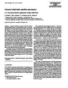
It is called a Keplerian velocity. The analytic expectation of circular motion is that, the last stable circular orbit for a particle moving around a Schwarzschild black hole in a Keplerian disk is at r = 6M (M is mass of black hole). Therefore, the gas or particles fall into the black hole, if their radial position is less than 6M . When their radial position is bigger than 6M , they should rotate in a circular orbit. Here, this problem is simulated and the numerical solution is compared to the analytic expectations. It tests the code with sources in the φ direction. In order to simulate this problem, the computational domain is chosen to be 3M ≤ r ≤ 20M and 0 ≤ φ ≤ 2π. The computational domain is filled with constant density and pressureless gas, rotating in circular orbits with the Keplerian velocity and zero radial velocity. In Fig. 12, the radial velocities of the gas vs. radial coordinate at different times are plotted. It is numerically observed that the gas inside the last stable orbit, r = 6M , falls into the black hole, while gas outside the last stable orbit follows circular motion with the Keplerian velocity as it is expected analytically. Fig. 13 shows the density of the fluid vs. radial coordinate at different times to see the behavior of the disk. It is seen that gas falls into the black hole for r < 6M . Accordingly, the numerical results from our code are consistent with the analytic expectations.
17 VII.
CONCLUSION
In this paper the Eulerian type numerical solution of general relativistic hydrodynamic equations constructed for relativistic astrophysics is presented. This code is constructed for general spacetime metric with lapse function and shift vector. It is capable of solving special relativistic problem and general relativistic problem coupling with the Einstein and hydrodynamic equations. This paper explains how general relativistic hydrodynamic equation can be solved with AMR. In the first part of the paper, the GRH equations and the numerical method are given. GRH equations are written in the conservative form and the numerical method and Paramesh package is applied to them with some appropriate way to get working code with AMR. Then, we have presented and tested solution of three-dimensional relativistic hydrodynamic equations using MUSCL scheme with Marquina fluxes. The results are obtained for problems involving relativistic flows, and strong shocks. These problems are solved using uniform and adaptive grid. Adaptive-Mesh Refinement is getting one of important technique in numerical relativity to solve the real astrophysical problems, such as accretion disks around the compact objects, and coalescing of the compact binaries. Adaptive-Mesh simulations pose many complex design problems, and a variety of different techniques that exist to solve these problems. The AMR is used to solve relativistic equations and to present some results from our numerical calculations. We solved the shock tube problem using different refinement levels to see the behavior of adaptive grid and also to compare AMR and uniform results with analytic solution. Results are converging to analytic solution when the number of resolutions are increased. Computing time used to solve AMR and uniform grid to get same accuracy are also compared. Results show that when the number of resolutions are increased AMR uses much less computing time than uniform grid. Finally, The full general relativistic hydrodynamical equation are tested using 2 − D test problems which are called free falling gas onto black hole and the circular motion of particles around the black hole. The numerical results from these test problems agree with analytic expectation and converge to analytic solution when the number of resolutions are increased. As a conclusion, AMR has permitted us to address problems of astrophysical interest which are really hard to solve with uniform grid. Because these problems are dominated by local physics, this code has been designed to handle highly relativistic flows. Hence, it is well suited for 2D and 3D simulations of astrophysical problems. First astrophysical results will be presented in a forthcoming paper for two-dimensional accretion disk problem around the black hole.
Acknowledgments
I would like to thank Joan M. Centrella for a great support and Peter MacNeice and Bruce Fryxell for a useful discussion. This project is supported by NSF PHY9722109 This project was carried out at NASA/GSFC, Laboratory of High Energy Astrophysics. It is also supported by NASA/GSFC IR&D. It has been performed using NASA super computers/T3E clusters..
References Banyuls, F., Font, J.A., Ibanez, J.M., Marti, J.M., and Miralles, J.A., Astrophys. J. 476, 221 (1997). Norman, M.L. and Winker, K.-H.A., in Astrophysical Radiation Hydrodynamics, edited by M. L. Norman and K.-H. A. Winkler (Reidel, Dordrecht, Holland, 1986). Font, J.A., Miller, M., Suen, W.-M., Tobias, M., Physical Review D, 61, 044011 (2000) Donat, R., Font, J.A., Ibanez, J.M., and Marquina, A., J.Comput. Phys. 146, 58 (1998). Misner, C.W., Thorne, K.S., Wheeler, J.A., Gravitation Schutz, B.F., in A First Course in General Relativity, edited by B. F. Schutz (Cambridge University Press, Cambridge, 1985). Ibanez, J.M., and Marti, J. JCAM (1998). Hirsch, C., in Numerical Computation of Internal and External Flows, edited by R. Gallagher and O. Zienkiewicz, Volume 2 (Wiley-Interscience, New York, 1992). Quirk, J., Int. J. Numer. Met. Fl. 18, 555-574, (1994).
18 Shu, C.W., Osher, S.J., J.Comput. Phys. 83, 32-78 (1989). Toro, E.F., Riemann Solver and Numerical methods for Fluid Dynamics, 1999. Bona, C., Masso, J., Seidel, E, and Walker, P., (1998), gr-qc/9804052. MacNeice, P., Olson, K.M., Mobarry, C., deFainchtein, R. and Packer, C., Computer Physics Communications, vo.126, p.330-354, (2000). Aloy, M.A., Ibanez, J.M., Marti, J.M., Muller, E., Astrophysical Journal Letters, 510, 119-122 (2000) Colella, P., and Woodward, P.R. J. Comput. Phys. 54, 174-201 (1984). Hawley, J.F., Smarr, L.L. & Wilson, J.R. 1984a, ApJ, 277, 296.
19
FIG. 1: Representation of adaptive-mesh refinement grid and tree structure. Figure is taken from MacNeice et al., 2000.
20
FIG. 2: Flux conservation is fixed at different refinement level boundaries. Figure is taken from MacNeice et al., 2000.
21
Shock Tube t = 0.4 analytic 32x32x32 64x64x64 128x128x128
density
1
0.5
0
0
0.1
0.2
0.3
0.4
0.5 r
0.6
0.7
0.8
0.9
FIG. 3: The analytic and numerical solutions of the relativistic shock tube problem for 3D.
1
22
0.25 error at each grid zone refinement levels Error, refinement level
0.2 coarsest level 0.15
0.1
0.05 finest level 0
0
0.2
0.4
0.6
0.8
1
r FIG. 4: Plotting the error and the refinement levels in each zone Eq.(43) is used as the refinement function with parameters: ctore(refinement parameter) = 0.035, ctode(derefinement parameter) = 0.005
23
0.25 error at each zone refinement levels error, refinement levels
0.2 coarsest level 0.15
0.1
0.05 finest level 0
0
0.2
0.4
0.6
0.8
1
r FIG. 5: Plotting the error and refinement levels in each zone. Eq.(44) is used as the refinement function with parameters: ctore(refinement parameter) = 0.035, ctode(derefinement parameter) = 0.005
24
0.25 error at each zone refinement levels error, refinement level
0.2 coarsest level 0.15
0.1
0.05
0
finest level
0
0.2
0.4
0.6
0.8
1
r FIG. 6: Plotting the error and refinement levels in each zone. Eq.(44) is used as the refinement function with parameters: ctore(refinement parameter) = 0.035, ctode(derefinement parameter) = 0.007
25
FIG. 7: Density is plotted in the x-y plane. Each square represents the block structure and each block has 8 points in a each direction. Eq.(44) is used as the refinement function with refinement parameters: ctore(refinement parameter) = 0.035, ctode(derefinement parameter) = 0.007.
26
lrefine_max=9, lrefine_min=3, nxb=8 1.5 error, 312 pts. 100*dx, 312 pts. corsest level 1
0.5
0
0
0.2
0.4
0.6
finest level 0.8 1
X FIG. 8: We plot the error and refinement levels in each zone to see the behavior of the refinement levels with errors. Eq.(44) is used as the refinement function with refinement parameters: ctore(refinement parameter) = 0.035, ctode(derefinement parameter) = 0.007.
Computing time per processor
27
Total numbers of processor used for all run are 64 20
Uniform AMR
t (hr)
15
10
5
0
0
50 100 grid zones along one side of cube
150
FIG. 9: The computing time for AMR and uniform grid runs of the 3D shock tube problem. The red line is the time per processor for AMR and the black line is the time per processor for uniform grid runs.
28
The fraction of the computational domain cover by the fine grid 1
Fine grid volume fraction
(a) 0.8
0.6
0.4
0.2
0
0
0.1
0.2 time
0.3
0.4
1 t = 0.1 t = 0.2 t = 0.3 t = 0.4
density
(b)
0.5
0
0
0.5 r
1
FIG. 10: (a): The fraction of the volume covered by the fines grid for AMR run of the 3D shock tube problem. (b): the density of the shock tube problem at different times.
29
0.9
2 numeric−256 analy
0.8 velocity
density
1.5 1 0.5 0
numeric−256 analy
0.7 0.6 0.5
2
4
6
8
10
8
10
0.4
2
4
6
8
10
radial velocity
−0.35 numeric−256 analy
−0.4 −0.45 −0.5 −0.55
2
4
6 r(M)
FIG. 11: The analytic solutions (red solid lines) with the numerical solutions (black circles) using 256 zones in the radial direction for thermodynamical variables, ρ, v, and v r .
30
0 t=100M t=50M t=25M t=12M t=0M
v^r( Radial Velocity)
-0.1
-0.2
-0.3
-0.4
-0.5
0
5
10
15
20
r(M) FIG. 12: Radial velocity vs. r is plotted. The radial velocity of fluid in the disk stays zero for r > 6M , during the evolution. r = 6M is called the last stable circular orbit in a Keplerian disk.
31
0.14 0.12
density
0.1 0.08 0.06 t=50M t=25M t=0M
0.04 0.02 0
0
5
10 r(M)
15
20
FIG. 13: Density vs. r is plotted. Density of the fluid is plotted at different times using different colors. The matter falls into the black hole while r is less than 6M .