As part of the publication [DS09], I started the design of a code generator for pairing ...... load it. The PHP code for the transmission is shown in Listing C.2.
Developing an automatic generation tool for cryptographic pairing functions Luis Julian Dominguez Perez B. Sc. M. A.
A Dissertation submitted in fulfilment of the requirements for the award of Ph.D. to the
Dublin City University Faculty of Engineering and Computing School of Computing
Supervisor: Michael Scott
January, 2011
Declaration I hereby certify that this material, which I now submit for assessment on the programme of study leading to the award of Ph.D. is entirely my own work, that I have exercised reasonable care to ensure that the work is original, and does not to the best of my knowledge breach any law of copyright, and has not been taken from the work of others save and to the extent that such work has been cited and acknowledged within the text of my work.
Signed: Luis Julian Dominguez Perez. ID: 57104328. Date: January 2011.
Abstract Pairing-Based Cryptography is receiving steadily more attention from industry, mainly because of the increasing interest in Identity-Based protocols. Although there are plenty of applications, efficiently implementing the pairing functions is often difficult as it requires more knowledge than previous cryptographic primitives. The author presents a tool for automatically generating optimized code for the pairing functions which can be used in the construction of such cryptographic protocols. In the following pages I present my work done on the construction of pairing function code, its optimizations and how their construction can be automated to ease the work of the protocol implementer. Based on the user requirements and the security level, the created cryptographic compiler chooses and constructs the appropriate elliptic curve. It identifies the supported pairing function: the Tate, ate, R-ate or pairing lattice/optimal pairing, and its optimized parameters. Using artificial intelligence algorithms, it generates optimized code for the final exponentiation and for hashing a point to the required group using the parametrisation of the chosen family of curves. Support for several multi-precision libraries has been incorporated: Magma, MIRACL and RELIC are already included, but more are possible.
Acknowledgements This research was sponsored by the Consejo Nacional de Ciencia y Tecnolog´ıa, Conacyt. Also thanks to the Claude Shannon Institute for its support and extra training. The extensive and key support from my supervisor has been fundamental to the realization of this research. Thank you so much Mike. Also, I would like to acknowledge all of the anonymous referees on my submitted and shared publications. Their feedback was also a key factor in the consummation of this project. From CSI, thanks to Gary, Marcus and all of the professors, post-docs and students for giving lectures and talks. A special thanks to Paulo Barreto for reading an early draft of this work. I would like to thanks to my friends from the lab. In particular to Naomi, for her outstanding support in proof-reading and joint-work. To Ezekiel for his support and the joint-work we had together. To Prof.. Kim for his extensive patience in the lab and his interesting talks. To Chen for always being there. To Rob for attending several times the same speech, and always giving feedback. To Denis for joining the cryptolab ship, and to Manuel. To Neil for proof-reading my thesis. And my friends from the bigger group: Brian, John, Richard, Danny, Geoff, and Jens, for that work and funny talks. Also, thanks for all the visitors. An special thanks to Diego F. Aranha and Juan Martinez Castillo, for his help on timing the code. A mis pap´as por apoyarme siempre en mis estudios, a mis hermanas y familiares, tanto tiempo perdido en familia. Y a mi abuelita (+) tambi´en I have had so many house-mates, you all make me happy, specially the 31ers. Hopefully we meet again.
Atentamente, Luis Julian.
TABLE
OF CONTENTS
List of Tables
vii
List of Figures
viii
List of Code
1
1
Introduction
1
2
Background
5
2.1
Elliptic Curves . . . . . . . . . . . . . . . . . . . . . . . . . . . . . . . .
5
2.1.1
Arithmetic of elliptic curves . . . . . . . . . . . . . . . . . . . . .
7
2.1.2
Tower extensions of finite fields . . . . . . . . . . . . . . . . . . .
9
2.1.3
Twist of a curve over an extension field . . . . . . . . . . . . . . .
11
2.1.4
ECDLP . . . . . . . . . . . . . . . . . . . . . . . . . . . . . . . .
12
2.1.4.1
Security level . . . . . . . . . . . . . . . . . . . . . . .
12
Elliptic Curve Isomorphisms . . . . . . . . . . . . . . . . . . . . .
14
2.2
Divisors . . . . . . . . . . . . . . . . . . . . . . . . . . . . . . . . . . . .
14
2.3
Cyclotomic Polynomial . . . . . . . . . . . . . . . . . . . . . . . . . . . .
15
2.4
Pairings . . . . . . . . . . . . . . . . . . . . . . . . . . . . . . . . . . . .
16
2.4.1
The Tate Pairing . . . . . . . . . . . . . . . . . . . . . . . . . . .
17
2.4.1.1
The Miller Loop for the Tate Pairing . . . . . . . . . . .
18
The ate Pairing . . . . . . . . . . . . . . . . . . . . . . . . . . . .
19
2.4.2.1
The Miller Loop for the ate Pairing . . . . . . . . . . . .
20
The R-ate Pairing . . . . . . . . . . . . . . . . . . . . . . . . . . .
22
2.4.3.1
Shorter R-ate pairing . . . . . . . . . . . . . . . . . . .
25
2.4.3.2
Choosing the R-ate pairing parameters . . . . . . . . . .
27
Pairing Lattices . . . . . . . . . . . . . . . . . . . . . . . . . . . .
28
2.1.5
2.4.2
2.4.3
2.4.4
i
Table of contents
2.5
2.6
2.7
2.8
2.9
2.4.5
Optimal Pairing . . . . . . . . . . . . . . . . . . . . . . . . . . . .
31
2.4.6
Comparison of the Miller-loop length . . . . . . . . . . . . . . . .
31
Pairing-Friendly Elliptic Curves . . . . . . . . . . . . . . . . . . . . . . .
32
2.5.1
MNT Curves . . . . . . . . . . . . . . . . . . . . . . . . . . . . .
33
2.5.2
Freeman Curves . . . . . . . . . . . . . . . . . . . . . . . . . . .
34
2.5.3
Barreto-Naehrig (BN) Curves . . . . . . . . . . . . . . . . . . . .
34
2.5.4
Kachisa-Schaefer-Scott Curves . . . . . . . . . . . . . . . . . . . .
34
2.5.4.1
KSS curves with k = 8 . . . . . . . . . . . . . . . . . .
35
2.5.4.2
KSS curves with k = 18 . . . . . . . . . . . . . . . . . .
35
2.5.4.3
KSS curves with k = 36 . . . . . . . . . . . . . . . . . .
36
Matrices . . . . . . . . . . . . . . . . . . . . . . . . . . . . . . . . . . . .
36
2.6.1
Greatest Common Divisor . . . . . . . . . . . . . . . . . . . . . .
36
2.6.2
Echelon Form . . . . . . . . . . . . . . . . . . . . . . . . . . . . .
36
Programming Languages . . . . . . . . . . . . . . . . . . . . . . . . . . .
37
2.7.1
Magma . . . . . . . . . . . . . . . . . . . . . . . . . . . . . . . .
37
2.7.2
MIRACL . . . . . . . . . . . . . . . . . . . . . . . . . . . . . . .
38
2.7.3
RELIC . . . . . . . . . . . . . . . . . . . . . . . . . . . . . . . .
38
Metaprogramming . . . . . . . . . . . . . . . . . . . . . . . . . . . . . .
39
2.8.1
Automatic Code Generation . . . . . . . . . . . . . . . . . . . . .
40
2.8.1.1
L- and R-value . . . . . . . . . . . . . . . . . . . . . . .
40
2.8.1.2
Suffix Notation . . . . . . . . . . . . . . . . . . . . . .
41
2.8.1.3
Operator Overloading . . . . . . . . . . . . . . . . . . .
42
2.8.2
Attribute-Oriented Programming . . . . . . . . . . . . . . . . . . .
43
2.8.3
Reflective Programming . . . . . . . . . . . . . . . . . . . . . . .
44
2.8.4
Template-based Metaprogramming . . . . . . . . . . . . . . . . .
45
Exponentiation in G2,T . . . . . . . . . . . . . . . . . . . . . . . . . . . .
46
2.9.1
Weak Popov Representation . . . . . . . . . . . . . . . . . . . . .
49
2.9.1.1
50
Popov Form . . . . . . . . . . . . . . . . . . . . . . . .
ii
Table of contents
2.9.2 3
Quasi-Echelon Form . . . . . . . . . . . . . . . . . . . .
51
2.9.1.3
Weak Popov Form . . . . . . . . . . . . . . . . . . . . .
52
The Galbraith-Scott Method using the Weak Popov Form . . . . . .
55
Addition Chains
57
3.1
Introduction . . . . . . . . . . . . . . . . . . . . . . . . . . . . . . . . . .
58
3.2
Bos and Coster Method . . . . . . . . . . . . . . . . . . . . . . . . . . . .
59
3.3
Binary Method . . . . . . . . . . . . . . . . . . . . . . . . . . . . . . . .
60
3.3.1
Construction of the Binary Method . . . . . . . . . . . . . . . . .
61
3.3.2
Example using the Binary Method . . . . . . . . . . . . . . . . . .
62
Artificial Intelligence method . . . . . . . . . . . . . . . . . . . . . . . . .
63
3.4.1
Artificial Immune System . . . . . . . . . . . . . . . . . . . . . .
64
3.4.1.1
Types of Cells on the Immune System . . . . . . . . . .
64
3.4.1.2
Immune Engineering . . . . . . . . . . . . . . . . . . .
65
3.4.1.3
Immune System Metaphors . . . . . . . . . . . . . . . .
65
Addition Chain Construction . . . . . . . . . . . . . . . . . . . . . . . . .
66
3.5.1
Initial Sequence Generation . . . . . . . . . . . . . . . . . . . . .
67
3.5.2
Auto-Immune Disease . . . . . . . . . . . . . . . . . . . . . . . .
68
3.5.3
Hypermutation . . . . . . . . . . . . . . . . . . . . . . . . . . . .
68
3.5.4
Core Function
. . . . . . . . . . . . . . . . . . . . . . . . . . . .
69
3.5.5
Results . . . . . . . . . . . . . . . . . . . . . . . . . . . . . . . .
72
3.6
Comparison of the Methods . . . . . . . . . . . . . . . . . . . . . . . . . .
72
3.7
Final Thoughts on Addition Chains . . . . . . . . . . . . . . . . . . . . . .
74
3.4
3.5
4
2.9.1.2
The Final Exponentiation
76
4.1
The Du, Hong and Pei Method . . . . . . . . . . . . . . . . . . . . . . . .
77
4.2
Devegili, Scott and Dahab Method . . . . . . . . . . . . . . . . . . . . . .
78
4.3
A new method . . . . . . . . . . . . . . . . . . . . . . . . . . . . . . . . .
79
4.3.1
86
More Examples . . . . . . . . . . . . . . . . . . . . . . . . . . . .
iii
Table of contents
4.4 5
6
4.3.1.1
The MNT curves . . . . . . . . . . . . . . . . . . . . . .
86
4.3.1.2
The BN Curves . . . . . . . . . . . . . . . . . . . . . .
87
4.3.1.3
Freeman Curves . . . . . . . . . . . . . . . . . . . . . .
89
4.3.1.4
The KSS:k = 8 Family of Curves . . . . . . . . . . . . .
90
A Note on the Final Exponentiation . . . . . . . . . . . . . . . . . . . . .
90
Fast Hashing to G2
92
5.1
Introduction . . . . . . . . . . . . . . . . . . . . . . . . . . . . . . . . . .
93
5.2
Point Counting . . . . . . . . . . . . . . . . . . . . . . . . . . . . . . . .
93
5.3
A new method . . . . . . . . . . . . . . . . . . . . . . . . . . . . . . . . .
96
5.4
Final Thoughts . . . . . . . . . . . . . . . . . . . . . . . . . . . . . . . . 101
Code Generator
103
6.1
Instruction Construction . . . . . . . . . . . . . . . . . . . . . . . . . . . 104
6.2
Attribute-based construction . . . . . . . . . . . . . . . . . . . . . . . . . 108
6.3
Reflective program construction . . . . . . . . . . . . . . . . . . . . . . . 109
6.4
Template-based construction . . . . . . . . . . . . . . . . . . . . . . . . . 111
6.5
Adding support to a library . . . . . . . . . . . . . . . . . . . . . . . . . . 112
6.6
6.5.1
Hashing to G2 [r] . . . . . . . . . . . . . . . . . . . . . . . . . . . 113
6.5.2
Final exponentiation . . . . . . . . . . . . . . . . . . . . . . . . . 114
6.5.3
The pairing function . . . . . . . . . . . . . . . . . . . . . . . . . 115
6.5.4
Others . . . . . . . . . . . . . . . . . . . . . . . . . . . . . . . . . 116
6.5.5
Linking the library to the project . . . . . . . . . . . . . . . . . . . 116
Parameters of the program . . . . . . . . . . . . . . . . . . . . . . . . . . 116 6.6.1
Other user-specified options . . . . . . . . . . . . . . . . . . . . . 117
6.7
Feedback symbols in the program . . . . . . . . . . . . . . . . . . . . . . 118
6.8
Code sequence . . . . . . . . . . . . . . . . . . . . . . . . . . . . . . . . 119 6.8.1
Default variables and functions load . . . . . . . . . . . . . . . . . 119
6.8.2
Sample generated code . . . . . . . . . . . . . . . . . . . . . . . . 126
iv
Table of contents
6.8.3 6.9 7
6.8.2.1
KSS k = 8 . . . . . . . . . . . . . . . . . . . . . . . . . 127
6.8.2.2
KSS k = 18 . . . . . . . . . . . . . . . . . . . . . . . . 130
Timings . . . . . . . . . . . . . . . . . . . . . . . . . . . . . . . . 141
Final Thoughts . . . . . . . . . . . . . . . . . . . . . . . . . . . . . . . . 145
Conclusions
146
A Example parameters of the curve
150
A.1 Hamming Weight . . . . . . . . . . . . . . . . . . . . . . . . . . . . . . . 150 B Certicom Challenge
151
B.1 Methodology . . . . . . . . . . . . . . . . . . . . . . . . . . . . . . . . . 153 B.2 Technical Requirements . . . . . . . . . . . . . . . . . . . . . . . . . . . . 154 B.3 Running the Attack from Ireland . . . . . . . . . . . . . . . . . . . . . . . 154 C Online Tutorial
157
C.1 Introduction . . . . . . . . . . . . . . . . . . . . . . . . . . . . . . . . . . 158 C.2 Magma Online Calculator . . . . . . . . . . . . . . . . . . . . . . . . . . . 159 C.3 AJAX . . . . . . . . . . . . . . . . . . . . . . . . . . . . . . . . . . . . . 160 C.4 YUI . . . . . . . . . . . . . . . . . . . . . . . . . . . . . . . . . . . . . . 162 C.4.1
YUI Structure . . . . . . . . . . . . . . . . . . . . . . . . . . . . . 162
C.5 Our Construction . . . . . . . . . . . . . . . . . . . . . . . . . . . . . . . 164 C.5.1
The XMLHttpRequest . . . . . . . . . . . . . . . . . . . . . . . . 165
C.5.2
Reading the Output . . . . . . . . . . . . . . . . . . . . . . . . . . 167
C.5.3
Displaying the Results . . . . . . . . . . . . . . . . . . . . . . . . 167
C.6 Internal Comparisons . . . . . . . . . . . . . . . . . . . . . . . . . . . . . 169 C.7 Final Thoughts about the Online Tutorial . . . . . . . . . . . . . . . . . . . 171 D Code Generator function list
172
Bibliography
180
v
Table of contents
Subject Index
196
vi
L IST
OF
TABLES
2.1
Tower extension construction . . . . . . . . . . . . . . . . . . . . . . . . .
10
2.2
Irreducible polynomials for the tower extension construction . . . . . . . .
11
2.3
NIST and ECRYPT security level recommendations . . . . . . . . . . . . .
13
2.4
KSS: k = 18 Curves A,B Parameters . . . . . . . . . . . . . . . . . . . . .
27
2.5
Comparison of Miller-loop length for a KSS:k = 18 curve, with Log2 x ≈ 63 32
3.1
Input Matrix for the Binary Method. . . . . . . . . . . . . . . . . . . . . .
62
4.1
Constructing the vector chain . . . . . . . . . . . . . . . . . . . . . . . . .
83
4.2
Partial final exponentiation code from the Olivos and Scott et al. method. KSS Curve:k = 18 . . . . . . . . . . . . . . . . . . . . . . . . . . . . . .
4.3
83
Partial final exponentiation code for the same curve, with a reduced number of ti elements. . . . . . . . . . . . . . . . . . . . . . . . . . . . . . . . . .
83
6.1
Filename Notation . . . . . . . . . . . . . . . . . . . . . . . . . . . . . . 109
6.2
Definitions for G2 . . . . . . . . . . . . . . . . . . . . . . . . . . . . . . . 113
6.3
Definitions for FE . . . . . . . . . . . . . . . . . . . . . . . . . . . . . . . 114
6.4
Definitions for pairing function . . . . . . . . . . . . . . . . . . . . . . . . 115
6.5
Timing the generated code . . . . . . . . . . . . . . . . . . . . . . . . . . 141
6.6
Comparison of the generated code, BN curves. CPU cycles in millions. . . 144
A.1 Useful Low Hamming-Weight Values . . . . . . . . . . . . . . . . . . . . 150 D.1 List of functions with Input/Output description . . . . . . . . . . . . . . . 173
vii
L IST
OF
F IGURES
2.1
Addition Operation . . . . . . . . . . . . . . . . . . . . . . . . . . . . . .
8
2.2
Doubling Operation . . . . . . . . . . . . . . . . . . . . . . . . . . . . . .
8
2.3
Point-at-Infinity . . . . . . . . . . . . . . . . . . . . . . . . . . . . . . . .
9
2.4
ψ map for KSS:k = 18 curves . . . . . . . . . . . . . . . . . . . . . . . .
21
2.5
ψ map for BN curves . . . . . . . . . . . . . . . . . . . . . . . . . . . . .
21
6.1
Feedback symbols . . . . . . . . . . . . . . . . . . . . . . . . . . . . . . . 118
C.1 Screenshot of the welcome screen. . . . . . . . . . . . . . . . . . . . . . . 159 C.2 Screenshot of the paginator . . . . . . . . . . . . . . . . . . . . . . . . . . 164 C.3 Screenshot of the Panel and Dialog . . . . . . . . . . . . . . . . . . . . . . 164 C.4 Screenshot of the displayed stored values . . . . . . . . . . . . . . . . . . 168 C.5 Screenshot of the Miller loop length computation for a random KSS:k = 8 curve. . . . . . . . . . . . . . . . . . . . . . . . . . . . . . . . . . . . . . 169 C.6 Screenshot of the R-ate pairing comparison . . . . . . . . . . . . . . . . . 170
viii
L IST
ψ via lifting, 44
OF
C ODE
Parsing the Magma Calculator, 167 Preparing the XMLHttpRequest, 165
Binary Method, 61 Display Computation, 167
Testing the Fast Cofactor Function, 110
Generic Assignment, 105
The XMLHttpRequest and Response,
GenericOperation, 106
166
1
1 I NTRODUCTION
”If it were ammunition, you would not be here.” – Gral. Pedro Maria Anaya after being asked to surrender the weapons and ammunition at the defense of the ’Convento de Churubusco’, August 20th, 1847.
I
NTEREST
in pairing-based cryptography has been growing since the arrival of the
new millennium, thanks to the development of many constructive protocols; for example, those given in [Jou00] and [BLS01]. The usefulness of these protocols
has caught the attention of industry. Traditional cryptographic protocols, such as RSA, are well established and seen as “secure enough” for the immediate future, but have limited functionality. Pairing-based cryptography is slowly being seen as a viable option. The main disadvantage of implementing pairing-based protocols instead of these wellestablished solutions is the deeper mathematical background required to produce an efficient implementation. Every year, new improvements on pairing computation methods appear. A pairing-based protocol designer may prefer to focus on the proof and formalization of the protocol itself rather than on the physical construction of the primitives upon which it relies. Given the many improvements, it is easy to lose track of the most “up-to-date” optimizations and use a less efficient implementation. This research in pairing-based cryptography started in a joint work of the author with Kachisa and Scott. This was an exploratory research, aiming to “get to know pairings” and to find possible areas for development. During that exploration, we were working with the recently discovered KSS:k = 18 family of curves looking for new properties of the curves. On the completion of a bilinear and non-degenerate pairing implementation, we noticed how slow it was; however, we were able to detect the cause, it was the infamous final ex-
1
Introduction
ponentiation. In an attempt to speed-up this step, we tried the [DSD07] implementation method for the BN curves. However, the implementation was not suitable for our purposes, as we failed to reproduce their results using our target curve. We commenced a joint work with Scott, Benger, Charlemagne and Kachisa [SBC+ 09b] to speed-up the Final Exponentiation operation for general pairing-friendly elliptic curves. It was our idea to use a base-p representation of the exponent as much as possible to find a pattern in the final exponentiation of the pairing. We tried simple exponentiation by factorization, as was suggested by the other authors, but we preferred a method making use of addition-chain theory. We developed a fast final exponentiation implementation that can be constructed for any family of pairing-friendly elliptic curves. This work resulted in a publication which was presented at the conference Pairing 2009. Switching focus to some operations necessary in pairing-based protocols, we noted yet another expensive operation: the scalar-point multiplication by a large cofactor. We applied the Galbraith and Scott [GS08] ideas for exponentiation in G2 groups to our problem for the family of curves we were originally working on. We developed a formal and faster method to hash a random point into a group G2 of order r. We were able to extend this method to other elliptic curves. This research was published in [SBC+ 09a]. Again, making use of the base-p representation of the curve parameters, and the Frobenius exponentiation, we added the map from Galbraith and Scott [Ibidem.] and obtained some promising results. We presented this work at Pairing 2009. This research is detailed in Chapter 5. Once these two issues had been solved, we decided to go back to explore implementation issues. This paper contained nothing new as we had already published the results separately. We simply compiled the results in one article and released it in the IACR eprint archive [DKS], where it has received much attention and has been referenced. The examples in the paper guide the reader through a tutorial which uses Magma software. We realized that not everybody has access to this software so, in order to reach a larger audience, I developed a webpage, where a user without a Magma license can follow the examples. The
2
Introduction
details of this online tutorial are explained in Appendix C. What seemed an unnecessarily complex algorithm, developed into a very useful method for finding addition sequences; we used the computer paradigm of Artificial Immune Systems to find the necessary sequences. In the work already described, we needed addition chains for the exponentiation in finite fields and for scalar-point multiplication in a group of points. As the embedding degree k, and the degree and complexity of the polynomials p and r defining the parameters of the curve grows, finding an addition sequence becomes unmanageable by pen-and-paper. I adapted the Cruz-Cortez et al. method [CCRHC08] to our addition sequences. A peer-reviewed paper which contains this modified method and some work from Scott was presented at the SPEED-CC 2009 Workshop [DS09]. As part of the publication [DS09], I started the design of a code generator for pairing functions. The afore mentioned publications and the new popularity of pairings functions requiring a construction method, needed be automatised. The aim of the code generator for cryptographic pairing functions is the following: to decide (or suggest) which family of pairing-friendly elliptic curves to choose (for example curves we refer to Freeman et al. [FST10, Table 1.1 and 8.3]); to find a low Hamming-weight x-parameter for the definition of the system parameters; to generate the elliptic curve with a subgroup size corresponding to the desired security level; to choose the pairing function that best suits the family of curves to which the chosen curve belongs, and its representation; to include supportive functions; and, optionally, to generate a sample “playground” for testing the code. In order for a code generator to be flexible, support for several multi-precision libraries should be included. Some characteristics of the code rely on the programming language itself; others rely on the library. Some operations use an in-fixed operator, depending on the library. For some, this may only be possible with the use of a map and with explicit intermediate storage, where for others, the compiler can handle it. Some recent speed records on the pairing computation are not based on a particular multi-precision library, but on a hand-crafted set of finite field arithmetic functions, such as: [NNS10, BGM+ 10, LMN10]. When referring to a multi-precision library in this research,
3
Introduction
we would like to include in the definition any set of specialised finite field arithmetic. We have a description of the code generator in Chapter 6. Our implementation paper is still alive and is highlighting interesting research areas. After the improvements given by the mentioned optimizations, in practical implementation of a pairing-based protocol [Sco02], the slowest part of the pairing function is now the exponentiation in the G2 and GT groups. As a side project, I have a contribution in an attempt to break a security system detailed in Appendix B, with the aim of developing an understanding of the real security of the detailed cryptosystems. The rest of this thesis is as follows: Chapter 2 gives a background on pairings, and metaprogramming for the techniques used in the code generator, Chapter 3 details the automatic construction of addition chains and the required computer science background. The conclusions and final remarks are presented in Chapter 7. Chapter 6 presents selected generated code; we stress that more sample code will be hosted on my personal webpage. Appendix A gives selected parameters for the pairing implementation.
4
2 BACKGROUND
”I am proud to be humble.” – Moises Castillo criticizing a spiritual leader.
T
HE
public release of the public key cryptosystem by Diffie and Hellman in
1976 [DH76] not only created modern cryptography, but also concentrated the Computational Number Theory efforts in this direction.
The first usable public key system was the RSA scheme introduced by Rivest, Shamir
and Adleman in [RSA78]; it is based on the problem of factoring large integers. Later, in 1985 Miller [Mil86], and independently Koblitz in [Kob87] pointed out a discrete logarithm problem (DLP) in the group of points of an elliptic curve defined over a finite field. A Public-Key Cryptosystem relies on the infeasibility of finding a decryption process given an encryption key. Elliptic Curve Cryptography (ECC), is a public-key cryptography system that uses the structure of the elliptic curves defined over finite fields [Sti95]. The main advantage of ECC is that it requires significantly smaller keys to encrypt/decrypt data, compared to other public-key cryptosystems, for similar security levels. It also scales better at higher security levels. The higher the security level, the better ECC compares with other public-key systems. This is particularly true when compared to cryptosystems based on RSA, which is the most widely used.
2.1
Elliptic Curves
Let p be a prime number, and Fp a field of integers modulo p. An elliptic curve E over the finite field Fp , denoted as E(Fp ), has its arithmetic in terms
5
Background
Elliptic Curves
of the underlying finite field and is defined by the following equation: y 2 = x3 + ax + b
(2.1)
where a, b are defined in Fp and satisfy 4a3 + 27b2 6≡ 0 mod p. The set of solutions (x, y) with x, y ∈ Fp satisfies equation 2.1. Additionally, the point-at-infinity, denoted as O or ∞ is also on the curve. Let P be a point in E(Fp ) with prime order r; then a cyclic subgroup of E(Fp ) generated by P is denoted as
< P >= {∞, P, 2P, 3P, . . . , (r − 1)P }
where r is the number of elements in the subgroup. Definition 1. The discriminant ∆(E) of an elliptic curve E is defined as [CF06]: ∆(E) = −16(4a3 + 27b2 )
where a,b are the parameters of the short Weierstrass formula of E. Definition 2. The absolute invariant, also known as the j-invariant of E, is defined as [CF06]: j(E) = 123
−4a3 . ∆(E)
Definition 3. Let E be an elliptic curve defined over Fp , then √ √ p + 1 − 2 p ≤ #E(Fp ) ≤ p + 1 + 2 p
is called the Hasse interval. The number of points on E(Fp ) is in the Hasse interval. The number t = p + 1 − #E(Fp ) is called the trace of Frobenius of E over Fp and satisfies √ |t| ≤ 2 p [HMV04].
6
Background
Elliptic Curves
Definition 4. The embedding degree of a curve is the smallest integer k where r|(pk − 1) and sometimes it is also referred as the security multiplier of the curve. Definition 5. An elliptic curve E defined over Fp is supersingular if p divides t, the trace of the Frobenius, otherwise the curve is ordinary [HMV04]. A supersingular curve with p > 3 has #E(Fp ) = p + 1. Definition 6. Let Fpk be an extension field of Fp of degree k. F∗pk is a field composed by the non-zero elements of Fpk under the multiplicative law. Definition 7. The Complex Multiplication method or simply CM method constructs an elliptic curve with a group of points with selected order r. The CM method is also referred to as the Atkin-Morain method for curves over prime fields; and the Lay-Zimmer method for curves over binary fields. This method is efficient if the finite field order p and the elliptic curve order r = p + 1 − t are selected so that the p complex multiplication field Q( t2 − 4p) has a small enough class number ([HMV04], pp. 179).
2.1.1
Arithmetic of elliptic curves
An elliptic curve E can be represented in several coordinate systems for instance, in [CF06, §13.2], a few of these systems are presented. Some of these systems reuse intermediate values in the arithmetic to gain a speed-up. Lauter, Montgomery and Naehrig in [LMN10] made an analysis of the affine coordinate system against some other projective coordinate systems which were thought in the literature to be faster. Their analysis covered the same type of computations as this thesis. Their findings suggest that, due to the simplicity of the affine coordinate formulae, it may be preferred. The following are the formulae for the group law for arithmetic on elliptic curves defined over Fp , using affine coordinates [CF06, 13.2.1.a].
Negation. Let P = (x1 , y1 ), then −P = (x1 , −y1 ).
7
Background
Elliptic Curves
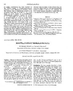
Figure 2.1: Addition Operation
Figure 2.2: Doubling Operation
Addition. Let P = (x1 , y1 ), and Q = (x2 , y2 ) such that P 6= ±Q, then P + Q = (x3 , y3 ).
y −y For an addition operation, set λ = 2 1 . x2 −x1
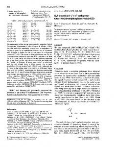
Doubling. Let [2]P = (x3 , y3 ). For a doubling operation, set λ =
3x21 +a 2y1
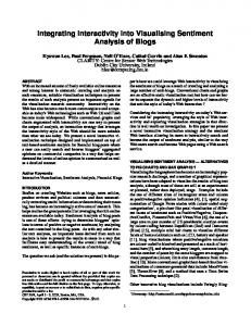
Then, we have x3 = λ2 − x1 − x2 , and y3 = λ(x1 − x3 ) − y1 . In the case of operations with the point-at-infinity: P + O = O + P = P .
Suppose we defined the elliptic curve over C instead of a finite field. Then the curve operations would be given geometrically as in Figures 2.1, 2.2 and 2.3, where λ is the slope of the line joining P and Q.
8
Background
Elliptic Curves
Figure 2.3: Point-at-Infinity
2.1.2
Tower extensions of finite fields
An element α ∈ Fpk can be represented as a polynomial up to degree k −1 with coefficients in Fp modulo an irreducible polynomial ∈ Fp [X]. For efficiency purposes, this irreducible polynomial should be simple. One method to construct the Fpk is using towers of extensions. Baktir and Sunar in [BS04] introduced the concept of tower field representation, which facilitates the finite field operations, in particular the inversion. They defined a tower field as a field obtained by extending its ground field with several irreducible polynomials. Benger and Scott in [BS09] presented a method to construct a tower, using toweringfriendly fields. Definition 8. A towering-friendly field is a field of the form Fqm , where q is a prime power, where q − 1 is divisible by all of the prime divisors of m.[BS09] These fields are constructed using a tower of sub-extensions using binomials as irreducible polynomials. Each sub-extension is a layer constructed by adjoining the roots of the previous level, this is, every other sub-extension is represented with elements of the previous sub-extension. The tower can be constructed using quadratic and cubic extensions of the previous base field until we reach the desired extension field (Fpk ). The table 2.1 presents the recommended choice of sub-extensions for selected embedding degrees [BS09]. The first column
9
Background
Elliptic Curves
k 8 12 18 24 36
Construction KSS 6.8 6.12 6.6 6.14
Tower 1-2-4-8 1-2-4-12 1-3-6-18 1-2-4-8-24 1-2-6-12-36
Table 2.1: Tower extension construction
is the k embedding degree, the second column is the name or the construction number of the family of elliptic curves from the Taxonomy paper [FST10]. The last column shows the degree of the extension fields to be constructed to get the final extension degree. For example, the first row in table 2.1 correspond to the KSS curves with k = 8. For this family, we construct a finite field Fp , on top of that, we construct a tower of extension fields in the following order: Fp2 , then Fp4 , and finally Fp8 . In [BN06] Barreto and Naehrig proposed the use of a polynomial X 6 − ξ, where 1/ξ = λ2 µ3 with λ ∈ Fp a non-cube, and µ ∈ Fp2 a non-square. Corollary 5 from the √ Benger and Scott method [BS09] says that a polynomial xm − (a ± b −1) is irreducible over Fp2 if a2 + b2 is neither a square nor a cube in Fp . We can trivially find either a small (a, b) or (λ, µ) pair with a linear search. Some of the values for (a, b) in the Benger and Scott paper are already calculated and are based on some values of p, the parameter defining the base field. See table 2.2 for a selection of the pairs. Column 4 from table 2.2 shows the (a, b) pair that can be used in the tower construction. Column 3 show the values for which column 4 is valid. Column 2 sets the degree of the irreducible polynomial. Column 1 lists the degree of the first tower, or the construction number on which the (a, b) pair applies.1 1
In the case of construction 6.12, since x ≡ 14 mod 42, x = 42.x0 + 14.
10
Background
Elliptic Curves
Fpn 2 2 Construction 6.8 6.8 6.8 6.12 6.12 6.12
Xm 2i 3j 2i 3j Xm 6 6 12 18 18 18
Test p ≡ 3 mod 8 p ≡ 2, 3 mod 5 Test x ≡ 7, 11 mod 12 x ≡ 1, 3, 7, 11, 12, 13 mod 15 x ≡ 1, 3, 7, 11, 12, 13 mod 15 x0 ≡ 1, 4, 5, 8 mod 12 x0 ≡ 7, 9, 12, 14 mod 15 x0 6≡ 2, 3, 4 mod 9
(a, b) (1,1) (2,1) (a, b) (1,1) (1,2) (5,0) (2,0) (5,0) (3,0)
Table 2.2: Irreducible polynomials for the tower extension construction
2.1.3
Twist of a curve over an extension field
A twist curve E 0 defined over Fpe , with e =
k d,
is another elliptic curve isomorphic to E
defined over Fpk . We define d as the degree of the twist of the curve E. The values of d, with a CM field √ defined as Q( D) are as follows [HSV06]: • d = 6 if the curve E has CM discriminant D = −3, and j(E) = 0. • d = 4 if the discriminant is D = −1, and j(E) = 1728. • d = 2 for any other value of D, and j(E) 6= 0, 1728. When d = 2, the curves is said to have or support a quadratic twist, when d = 3: cubic twist, when d = 4: quartic twist, and when d = 6: sextic twist. The formulae for an elliptic curve E is y 2 = x3 + a.x + b, defined over Fp , whereas the formulae for the twisted curve E 0 depends on the degree of the twist, and are as follows: E 0 : y 2 = x3 + 1/D2 ax + 1/D3 b
for d = 2 :
E 0 : y 2 = x3 + 1/Dax
for d = 4
E 0 : y 2 = x3 + 1/Db
for d = 6
where D ∈ Fpe such that W d − D is irreducible over Fpe [W ].
11
Background
Elliptic Curves
Furthermore, if δ ∈ Fpk is a root of W d − D , then there exists a homomorphism which maps points on the twist E 0 to the points of the curve E as follows: ψ : E 0 (Fpk/d ) → E(Fpk ) defined by: (x0 , y 0 ) → (x0 .δ 1/3 , y 0 .δ 1/2 ), with an isomorphism given by: φ : µd → Aut(E) : δ 7→ [δ] with [δ](x, y) = (x.δ 2 , y.δ 3 ) [HSV06]. One way to compute this map is by pre-computing δ 2 , δ 3 .
2.1.4
ECDLP
The Elliptic Curve Discrete Logarithm Problem (ECDLP) may be described as follows: Given an elliptic curve E defined over a finite field Fp , a point P ∈ E(Fp )[r], and a point Q in the group of points generated by P , find the integer n ∈ [0 . . . r − 1] such that Q = nP . The integer n is called the discrete logarithm of Q with respect to P . The hardness of the ECDLP is essential for the security of all elliptic curve cryptographic schemes [HMV04]. Computing nP should be easier than finding n (solving the discrete log), otherwise the system can be easily comprised. On the another hand, the cost of finding n should be significantly greater than the value of n. One way to find n is by a linear search: R = P , for n = 0 to r − 1: R+ = P until R = Q. For sufficiently large values of r there is no feasible algorithm to find n. Appendix B gives details of an attack to finding n for a “sufficiently large” value of r. 2.1.4.1
Security level
The main concern about the security of a system, is how long does an attacker need to break it, and how many resources are needed. The cost of breaking a system, measured both in time and in money invested in computational resources, should be greater than the value of the protected information. For example, if an attacker would need the equivalent of one million Euro to get access to an asset worth a hundred Euro, we presume that the attacker would cease on his attempt.
12
Background
Elliptic Curves
Equivalent symmetric key size Log2 (Fpk ) NIST Log2 (r) Log2 (Fpk ) ECRYPT Log2 (r)
80 1024 160 1248 160
112 2048 224 2432 224
128 3072 256 3248 256
192 7680 384 7936 384
256 15360 512 15424 512
Table 2.3: NIST and ECRYPT security level recommendations
When we say that an attacker would need 100 years to break the security of a system, it is usually calculated with the computational resources available at the start of the attack. As the time passes, newer, faster and cheaper computational resources appear; an attacker can be upgrading its computational resources during the attack, reducing the initial 100 years attack into a smaller number of years. On symmetric cryptographic schemes, the lifetime of the protection of the data can be calculated straight-forward by the time it would take to break the security by brute force, guessing or other attack, and including the improvements on computational power during the time of the attack. The traditional RSA cryptosystems has its hardness based on the integer factoring problem. In the case of elliptic curve cryptography, the hardness is based on the discrete log of elliptic curve groups defined over finite fields. It is traditionally suggested than elliptic curve in a subgroup of size m-bit is equivalent to a m/2-bit symmetric key. In [NIS] NIST states that an 80-bit symmetric key is equivalent to a 160-bit one using discrete logs subgroups and elliptic curve groups. This is defined as a 80-bit security level, and it is not recommended for use after 2012. An 128-bit security level is recommended therefore after that year. The ECRYPT network also publishes its own recommendations [ECR]. Table 2.3 shows the NIST and the ECRYPT recommendations of the pairing-friendly subgroup and the size of the finite field extension for several security levels.
13
Background
2.1.5
Divisors
Elliptic Curve Isomorphisms
Definition 9. The ring of endomorphisms of E, defined over Fp is denoted by EndFp E. For any integer n, the multiplication-by-n map P 7→ [n]P is an endomorphism of E. Definition 10. The Frobenius endomorphism, denoted πp , is the mapping given by [Men93]: πp : E 7−→ E : (x, y) 7−→ (xp , y p ) satisfying πpk (Q) = Q for any Q ∈ E(Fpk ). Definition 11. An efficiently computable homomorphism: ψ i = φ−1 πpi φ, where φ : E 0 (Fpk/d ) → E(Fpk ) is the isomorphism which takes a point from the twisted curve E 0 (Fpk/d ) to the isomorphic group on E(Fpk ), and π is called the p-power Frobenius map on E. Then ψ : φ−1 πφ is an endomorphism ψ : G02 (E 0 ) → G2 (E), where G02 and G2 are the group of points on the twisted curve and on the elliptic curve over the extension field respectively.
2.2
Divisors
We recall the following definitions from [Sil86]: Definition 12. The divisor group of a curve C, denoted Div(C), is the free Abelian group generated by the points of C. Thus a divisor D ∈ Div(C) is the formal sum:
D=
X
nPi (P ).
Pi ∈C
with nPi ∈ Z and nPi = 0 for all but finitely many P ∈ C. Definition 13. The degree of D is defined by
deg D =
X Pi ∈C
14
nPi .
Background
Cyclotomic Polynomial
Definition 14. The divisors of degree 0 form a subgroup of Div(C), denoted as: Div0 (C) = {D ∈ Div(C) : deg D = 0}.
Definition 15. If C/K, then GK/K acts on Div(C) and Div0 (C) as ¯ Dσ =
X
nPi (P σ ).
Pi ∈C
It follows that D is defined over K if Dσ = D for all σ ∈ GK/K . ¯ ∗ . The divisor div(f ) of f is given ¯ Definition 16. Let C be a smooth curve and f ∈ K(C)
by div(f ) =
X
ordPi (f )(P ).
Pi ∈C
Definition 17. A divisor associated to a function is called the principal divisor. The set of principal divisors forms a group PrincC . The div(f ) can be represented as the difference of the following divisors:
div(f ) = div(f )0 − div(f )∞ .
the points in div(f )0 with non-zero coefficients are called zeroes. Similarly, the points in div(f )∞ with non-zero coefficients are called the poles.
2.3
Cyclotomic Polynomial
The nth cyclotomic polynomial Φn (x) is defined to be Π(x − ζ), where ζ ranges over the primitive nth roots of unity in C. Definition 18. The Euler totient function, represented as ϕ is:
ϕ(N ) = |{x|1 ≤ x ≤ N, gcd(x, N ) = 1}|.
15
Background
Pairings
The Φn (x) is an irreducible polynomial in Z[x]. The deg Φn (x) = ϕ(n) [LL96]. P The irreducible factorization of xt − 1 in Z[x] is given by xt − 1 = d|t φd (x), where φd (x) is the dth cyclotomic polynomial. The factor φt (x) is the only irreducible factor xt −1 that does not appear in the factorization of xs − 1 for divisors s of t with s < t [Len97].
2.4
Pairings
Originally there were two pairings used in cryptography, the Weil and Tate-Lichtenbaum pairings, both evaluated using the Miller Algorithm. The Weil pairing requires two Miller loops to generate the rth roots of unity [Sil86, III.§8], while the Tate pairing requires an exponentiation of a single application of the Miller loop [Hes08], making it more efficient than the Weil pairing [GPS06]. The Miller Algorithm uses lg(r − 1) iterations. It uses a double-and-add, and a lineand-tangent approach. The basic Miller loop is presented in Algorithm 1, and explained in the following. Algorithm 1 Basic Miller loop Input: P, Q ∈ E(Fp )[r], P 6= Q and l ∈ N Output: f ∈ E(Fp ) T ←P f ←1 i ← blg2 (l) − 1c for i = 0 to l − 1 do f ← f 2 · lT,T (Q)/v[2]P (Q) T ← [2]P if li = 1 then f ← f · lT,P (Q)/vT +P (Q) T ←T +P end if end for return f
16
Background
2.4.1
Pairings
The Tate Pairing
The Tate pairing was introduced by Tate as a rather general pairing on Abelian varieties over local fields. Lichtenbaum gave an application of this pairing to the Jacobians of curves over local fields. The Tate-Lichtenbaum pairing is hereafter referred to as the Tate pairing. [CF06] Let P ∈ E(Fp )[r] and Q ∈ E(Fpk ), and consider the divisor D = (Q + S) − (S) with S a random point in E(Fpk ). Let fa,P be a function with a divisor (fa,P ) = a(P ) − (aP ) − (a − 1)(0)
for a ∈ Z. A non degenerate, bilinear Tate pairing is the map: er : E(Fp )[r] × E(Fpk )/rE(Fpk ) → F∗pk /(F∗pk )r (P, Q) 7→ fr,P (Q) The value of the pairing is in an equivalence class, F∗pk /(F∗pk )r . For practical purposes it is preferred to raise the value of the pairing to the power of (pk − 1)/r ∈ F∗pk to obtain a unique representative of the class, and to make it bilinear [Hes08]. This exponentiation is known as the final exponentiation, and the pairing is referred to as the Reduced Tate Pairing. The Tate pairing becomes: er (P, Q) : (P, Q) 7→ fr , P (Q)(p
k −1)/r
.
(2.2)
The focus of Chapter 4 will be on how to speed-up this operation. We define the G1 ∈ E(Fp )[r] as the group of points of order r on E over the base field Fp , and G2 as the group on E(Fpk )/rE(Fpk . Let P be a point in G1 and Q a point in G2 .
17
Background
2.4.1.1
Pairings
The Miller Loop for the Tate Pairing
Implementing the Tate Pairing is almost as easy as implementing the Miller loop. A straightforward method for implementing the Miller’s algorithm is explained in [BLKS02, Theorem 2] and [Sco07]. For each pair A, B ∈ E(Fp ), we define gA,B : E(Fpk ) → Fpk as the equation of the line through the points A, B to the curve E(Fpk )[BLKS02]. The code in Listing 2.1 computes the line function lA,B (Q), where A, B are two points on the curve E(Fp ), and a point Q on the curve E defined over the extension. This function is required to evaluate the contribution to the pairing value of the elliptic curve point addition, A + B. In essence these are distances calculated between the fixed point Q and the lines that arise when adding points A and B. In this code there are three cases to be considered. Listing 2.1: Line function code in Magma //Input return in G_T L:= function(A,B,Q) if A eq -B then return Q[1]-A[1]; end if; if A eq B then lambda:=(3*A[1]ˆ2+a) / (2*A[2]); else // A ne B lambda:=(B[2]-A[2])/(B[1]-A[1]); end if; return (lambda*(Q[1]-A[1]) + A[2]-Q[2]); end function;
The first case is where A = B, the line passing through this point is the tangent to the curve at point A the second case is when A 6= B. These two cases use the following operation: (lambda * (Q[1] - A[1]) + A[2] - Q[2]), where lambda is the slope of the line. The last case is when the point A is a negative of point B. In this case we have a vertical line and we compute Q[1] - A[1]. Refer to [Sil86] or [BLKS02] for more details. In practice, the equation of the curve, defined with a tuple (a, b) ∈ {(−3, b), (0, b 6=
18
Background
Pairings
0), (a 6= 0, 0)} is preferred as it simplifies the line function operations. The full Tate Pairing algorithm is presented in Listing 2.2. In this code the double-andadd stages can be identified by a 2 ∗ T (double) and a T + P (add), where the addition is required when a 1 (a pole) is present in the binary expansion of r. Additionally, there is the “vanilla” implementation of the final exponentiation step, using direct exponentiation. Listing 2.2: Basic Tate pairing with single Miller Loop // Input f \in G_T pairing:= function(P,Q) f:=1; T:=P; i:=Floor(Log(2,r))-1; si:=Intseq(r,2); while i ge 0 do f:=fˆ2*L(T,T,Q); T:=2*T; if si[i+1] eq 1 then f:=f*L(T,P,Q); T:=T+P; end if; i:=i-1; end while; f:=fˆ(((pˆk)-1) div r); return f; end function;
2.4.2
The ate Pairing
The ate pairing [HSV06] is a variant of the Tate pairing and it is a generalization of the Eta pairing, a pairing that can be used with supersingular elliptic curves [BGHS07]. The ate pairing is particularly suitable for pairing-friendly curves with small values of t. We take G1 = E[r] ∩ Ker(πp − [1]) and G2 = E[r] ∩ Ker(πp − [p]), and let T = t − 1. Let N = gcd(T k − 1, pk − 1) and T k − 1 = LN . For Q ∈ G2 and P ∈ G1 , the ate pairing is defined as [HSV06]: k −1)/N
eT : (Q, P ) 7−→ fT,Q (P )cT (p where cT =
Pk−1−i i=0
,
pi ≡ kpk−1 mod r. The ate pairing is a bilinear, non-degenerate
19
Background
Pairings
pairing if r - L. There is a switch in the arguments with respect of the Tate pairing; the first parameter Q is defined over the extension field and P is defined over the base field. We can always use the traditional final exponentiation (pk − 1)/r if T k 6≡ 1 mod r2 , since r|N and r - c the function is always bilinear, and non-degenerate as a result of Theorem 2 of [Hes08].
2.4.2.1
The Miller Loop for the ate Pairing
The number of iterations in the ate pairing in the Miller loop depends on the size of the trace of the Frobenius t rather than on the size of the subgroup r. As a result, if (ω = log r/ log |t|) > 1 for a particular family then it is possible to compute the ate pairing faster than the Tate pairing for that family of curves [Sco07]. The larger the value of the ω the faster the ate pairing computation is compared to the Tate pairing computation. For example, the KSS curves with embedding degree k = 18 have ω = 3/2, and so, this curve is suitable for an implementation of the ate pairing. The code in Magma for computing the ate pairing is given in Listing 2.3, where G1 ∈ E(Fp )[r]) and G2 ∈ E 0 (Fp3 ). Note that here we define G2 on the sextic twist. Listing 2.3: ate pairing with single Miller Loop //Input f \in $G_T$ pairing:= function(P,Q) f:=1; T:=P; s:= t-1; i:=Floor(Log(2,s))-1; si:=Intseq(s,2); while i ge 0 do f:=fˆ2*L(T,T,Q); T:=2*T; if si[i+1] eq 1 then f:=f*L(T,P,Q); T:=T+P; end if; i:=i-1; end while; f:=fˆ(((pˆk)-1) div r); return f; end function;
20
Background
Pairings
In the Miller loop, however, some operations on the curve over the extension field are required; in the case of the ate pairing it is the line function. Since one is using a point Q ∈ E 0 (Fpk/d ) instead of E(Fpk ), it is therefore required to apply the map ψ, discussed in §2.1.5, in the line function. Figure 2.4: ψ map for KSS:k = 18 curves
Each of the x and y coordinates of a point Q ∈ E 0 (Fp3 ) has three components defined over the base field Fp . A point in a curve E(Fp18 ) has six components of Fp3 , or eighteen of Fp . Instead of applying the map function ψ, one can move the x and y-coordinates of Q to their corresponding positions in a point in a curve E(Fp18 ), and apply the Frobenius exponentiation part there. A similar approach can be taken for the BN curves: Figure 2.5: ψ map for BN curves
Unfortunately, this cannot be done in Magma, and we don’t have this transformation for other families of curves. Instead we apply the “full” ψ map operation (x, y) 7→ (x.δ 2 , y.δ 3 ). Since δ is a constant for the generated curve, we can pre-compute these values and the cost of the mapping will be just one multiplication by a coordinate component (each time the line function in Listing 2.1 is called.) Listing 2.4 shows the corresponding code for the Line function. Listing 2.4: Line Function with ψ map //Input return in G_T
21
Background
Pairings
L:= function(A,B,Q) Ax:=A[1]*deltas[1]; Ay:=A[2]*deltas[2]; Bx:=B[1]*deltas[1]; By:=B[2]*deltas[2]; if (Ax eq Bx) then if (Ay eq -By) then return Q[1]-Ax; else if (Ax eq Bx) and (Ay eq By) then lambda:=(3*Axˆ2+a) / (2*Ay); end if; end if; else // A ne B lambda:=(By-Ay)/(Bx-Ax); end if; return (lambda*(Q[1]-Ax) + Ay-Q[2]); end function;
Alternatively, if δ ∈ E(Fpk/d ) already, then we do not need to lift the element from the twisted curve to the curve over the extension field to apply the map.
2.4.3
The R-ate Pairing
The R-ate pairing introduced by Lee, Lee and Park [LLP08], is a generalization of the ate [HSV06] and atei [ZZH07] pairing, improving the computation efficiency. It takes three short Miller loops to calculate the pairing, that together require a shorter loop than a single typical application of the Tate or the ate pairing. The R-ate pairing can be regarded as a ratio of two pairings, hence the name. Corollary 3.3 from [LLP08] defines four combinations of the R-ate pairing. Combination 1 matches the Miller loop length of the atei pairing. Combination 2 requires a Miller loop length of the field size, which is not optimal. Combination 4 matches the Miller loop length of the Tate pairing. In this research, we prefer the R-ate pairing option 3 since we can achieve the smallest number of Miller loops, and from now on, we refer to it simply as the R-ate pairing, unless specified. The R-ate pairing, like the atei [ZZH07], requires the calculation of Ti ≡ pi mod r, with 0 ≤ i < k, where k is the embedding degree. This pairing is constructed from the parameters (p, r), which are also used to define the ate and Tate pairing, and a combination
22
Background
Pairings
of the Ti s. The definition of the R-ate pairing with A = aB + b where A = Ti , B = Tj , and a, b, ∈ Z is as follows: eA,B (P, Q) : (P, Q) 7→ fa,BP (Q) × fb,P (Q) × GaBP,bP (Q) Generally this equation does not automatically give a bilinear and non-degenerate pairing. However, with a careful choice of pairs A and B, this is possible. For efficiency, we look for a working and non-trivial combination of A and B that gives the shortest Miller loop. In [LLP08, Algorithm 2] there are three Miller loops to compute and the final exponentiation is calculated at the end of the computation. The code for the Miller loop denoted as M in Listing 2.5 can be used to compute the R-ate pairing. It makes function calls to Listing 2.1, the line function. Listing 2.5: Miller loop as to be used by the R-ate pairing // Input f \in G_T, T \in \Z M:= function (P,Q,l) T:=P; f:=1; i:=Floor(Log(2,l))-1; li:=Intseq(l,2); while i ge 0 do f:=fˆ2*L(T,T,Q); T:=2*T; if li[i+1] eq 1 then f:=f*L(T,P,Q); T:=T+P; end if; i:=i-1; end while; return f,T; end function;
Listing 2.7 shows an implementation of the R-ate pairing function. As described in [LLP08, Algorithm 2], we denote fa , fb , aQ and bQ as {a, b} = {m1,m2}, where m1 and m2 are as follows: m1 = max{a, b} and m2 = min{a, b}. The R-ate pairing is also denoted as RA,B (P, Q). For the KSS k = 18 curve the linear
23
Background
Pairings
combination: T13 =
3x 7 .T6
+
2x 7 ,
where a =
3x 7 ,j
= 6 and b =
2x 7
gives the shortest
bilinear and non-trivial R-ate pairing. 1 We know from [LLP08, Algorithm 2] that c ← [ m m2 ] and d ← m1 − c × m2 . For
the a and b values proposed, we set d =
a 2.
With these values, the first and third Miller
function call can be integrated into one as shown in Listing 2.6. This is a good choice since A and B have almost the same number of bits with both values less than the x-parameter, the parameter of the curve, and as such, it provides a short Miller length of which one can use an intermediate value of f and T from Listing 2.5 to reuse computation. Listing 2.6 presents the optimised Miller’s loop for the R-ate pairing reusing partial results. Listing 2.6: Modifications to the Miller loop for the R-ate pairing // Input f \in G_T, T \in \Z M:= function (P,Q,l) T:=P; f:=1; i:=Floor(Log(2,l))-1; li:=Intseq(l,2); while i ge 0 do f:=fˆ2*L(T,T,Q); T:=2*T; if li[i+1] eq 1 then f:=f*L(T,P,Q); T:=T+P; end if; if i eq 1 then f2:=f; T2:=T; end if; i:=i-1; end while; return f,T,f2,T2; end function;
Since the parameters of the first and the third Miller loop are the same exempt the loop length, we only need to verify that d is equal to the most significant bits of m2. Unless this condition is met, we use either twice the function at Listing 2.5 or a single execution of the function at Listing 2.6. Another interesting characteristic of the selected combination is that if c = 1, we also avoid some computations. Furthermore, one can omit unnecessary use of memory since by
24
Background
Pairings
definition; a, b, j, m1, m2, c, d, fcm2 and cm2Q are known in advance. Listing 2.7: R-ate pairing function // Input f \in G_T, T \in \Z pairing:= function(P,Q) dd:=(xx) div 7; m1:=(3*dd); m2:=(2*dd); jj:=6; //Compute fm2,m2Q,fd,dQ:=M(Q,P,m2); f1:=fm2*fd; fm1:=f1*L(m2Q,dQ,P); m1Q:=m2Q+dQ; //Exponentiation f2:=Frobenius(fm1,Fp,jj)*fm2; Q1:=[Frobenius(m1Q[1]*V2,Fp,jj),Frobenius(m1Q[2]*V3,Fp,jj)]; Q1:=ExtT![Q1[1]*V1_2,Q1[2]*V1_3]; f3:=f2*L(Q1,m2Q,P); //Final Exponentiation f3:=f3ˆ(((pˆk)-1) div r); return f3; end function;
The code, “fm2,m2Q,fd,dQ:= M(Q,P,m2)”, in the Compute section of Listing 2.7 returns fm2 as f and m2Q as T in Listings 2.5 or 2.6. Clearly Q and m2 are the parameters of the M function, where m2 is the Miller loop length. Hence m2Q is the actual state of T. Additionally, since there is only one M function call, one would be able to insert the Miller loop inside a modified version of the Listing 2.7 to avoid overhead at runtime. Finally, Q1 ∈ E(Fp18 ) and the line function requires it to be in the twisted curve E 0 (Fp3 ); hence, we apply the inverse ψ map from §2.1.5 before the line function.
2.4.3.1
Shorter R-ate pairing
Recalling notation from [LLP08], to evaluate the R-ate pairing, the generic algorithm can be used. Then, the overall shortest Miller loop can be constructed as follows:
25
Background
Pairings
The three Miller loop calls are:
M (Q, P, m2 )
(2.3)
M (m2 Q, P, c)
(2.4)
M (Q, P, d)
(2.5)
where the parameters for these Miller function calls are as follows:
m1 ← max{a, b};
(2.6)
m2 ← min{a, b}; � � m1 ; c← m2
(2.7)
d ← m1 − c · m2 .
(2.8) (2.9)
and M is the Miller function. If an (A, B) pair is chosen such that the parameters are close to each other, then the ratio can be 1 (or close to 1), leaving one Miller loop that does not require execution as the result can be known in advance2 . The other two function calls can be embedded inside each other to use a partial result from the computation [DKS, Listing 15]. On the another hand, if the chosen parameters have a high ratio, some speed improvement is still possible. For example, some of the intermediate values of the R-ate pairing can be computed in parallel. This is not always possible for all of the families of pairingfriendly curves and still a smaller ratio on the parameters should be faster than distributed loops. Additionally, in our best effort, there are no family of curves for which the Ti ,Tj combinations suggest that it is possible to compute two parallel Miller loops instead of one short loop, and gain speed 3 . For example, we examine the case of the KSS curves with embedding degree k = 18 2
we can at least simplify the code If the third Miller loop needs to be embedded into the first one, it means that we need the second Miller loop, otherwise the first loop is not needed 3
26
Background
Pairings
# 1 2 3 4 5 6 7 8 9 10 11 12 13
a 3 5x/7 3x/7 5x2 /49 5x2 /49 5x/14 8x2 /49 3x/7 2x/7 3x/14 8x2 /49 3x2 /49 3x2 /49
Miller-length in iterations b Tj loops Ham x 1 64 30 x2 /7 1 187 85 2 2x /7 1 186 90 3x2 /49 3 246 119 8x2 /49 6 247 125 3x2 /14 16 186 88 3x2 /49 6 247 119 2x/7 6 62 22 3x/7 12 62 22 x2 /14 7 184 89 2 5x /49 12 247 125 8x2 /49 12 247 119 2 5x /49 15 246 119
m2 1 63 62 123 124 62 123 62 62 61 124 123 123
c 62 61 63 0 0 63 1 0 0 62 0 1 0
d 1 63 61 123 123 61 123 61 61 61 123 123 123
Table 2.4: KSS: k = 18 Curves A,B Parameters
[KSS08] in Table 2.4 with a subgroups size of approximately 192-bits. The first and second columns give the a and b parameters from Ti = a.Tj + b. The ‘loops’ column presents the total number of loops necessary for the R-ate pairing computation. The columns ‘m2 ’ and ‘c’ represent the parameters of the Miller loop in bits (as given in formulæ 2.3 and 2.4). The column ‘Ham’ shows the Hamming-weight of the length of the Miller loops. We see in Table 2.4 that for the example illustrated above, there are several (A, B) pairs which already have the shortest Miller loop length: row 8 and 9. These are our recommended parameters for the R-ate pairing. As mentioned before, other families of pairing-friendly elliptic curves may present favourable ratios and this feature (parallel execution) can be exploited. Generating code for parallel computation is left as a future option.
2.4.3.2
Choosing the R-ate pairing parameters
Choosing the length parameters of the R-ate pairings is an easy task that requires the p(x) and r(x) parameters of the desired curve. See Algorithm 2. Once the Ti polynomials are generated, it is necessary to verify the bilinearity and non-
27
Background
Pairings
Algorithm 2 Generate the Ti − Tj combinations for i = 0 to k − 1 do Polyi ← pi mod r � Discard Polyi ∈ [1,-1] for j = i + 1 to k − 1 do � Discard Polyj ∈ [1,-1] � Discard negative A,B components � Discard trivial combinations Poly Ai ← [ Poly i ] j Bi ← Polyi mod Polyj Ti ← i Tj ← j end for end for degeneracy properties of the R-ate pairing with the given parameters. We stress that the R-ate pairing requires an exponentiation to the parameter c from Equation 2.8; hence, when constructing the pairing, we may prefer to have a smaller footprint in favour of a slightly longer Miller loop. For example, the first row of table 2.4 is almost as short as row 8 and 9 but this selection would require an exponentiation of a number of approximately 62 bits.
2.4.4
Pairing Lattices
The family of ate pairings [HSV06, GHO+ 07, ZZH07, MKHO07] are optimized versions of the Tate pairing restricted to the eigenspaces of the Frobenius. P Let s ∈ Z, h = di=0 hi xi ∈ Z[x] with h(s) ≡ 0 mod r and d = ϕ(k), with k the embedding degree, and Q ∈ E(Fpk )[r], then:
(fs,h,Q ) =
d X
hi ((si Q) − (O)).
i=0
Defining ||h||1 =
Pd
i=0 |hi |
we have that if s is a primitive k th root of unity modulo r2 ,
28
Background
Pairings
and if h(s) ≡ 0 mod r but h(s) 6≡ 0 mod r2 , then, es,h : (Q, P ) 7→ fs,h,Q (P )(p
k −1)/r
defines a bilinear and non-degenerate pairing [Hes08].
Choosing s For the choice of s, following the ate pairing definition, we can take s = r, the subgroup size, but we prefer to take s = T = t − 1, which is already an improvement with respect to the Tate pairing.
Constructing h For the case of h, we construct a matrix m × m, with m = ϕ(k): M =
r
0
···
0
−T
1 0 ··· 0
−T 2 .. .
0 1 ··· 0 .. .. . .
−T m−1 0
···
1
Let w = (w0 , w1 , . . . , wm−1 ) be the shortest Z-linear combination of the rows of M , P i then we can construct h = m−1 i=0 wi x . In [Hes08], the author suggest to LLL-reduce the matrix M to get the shortest vector. To find the expansion with short coefficients, in [Ver10] Vercauteren uses the “ShortestVectors()” Magma function. A method to get vectors of lower degree is by transforming the matrix to have the Weak Popov Form using Algorithm 3. The explicit pairing lattice is defined as:
(Q, P ) 7→
l Y i=0
pi
fci ,Q (P ) ·
l Y
!(pk −1)/r G[si+1 ]Q,[ci qi ]Q (P )
i=0
29
Background
where si =
Pairings
Pl
j=i cj p
j,
G is the line function, and k is even.
For the construction, note that: f1,Q = 1, f−1,Q = 1/f1,Q (for k odd), and [1/2]Q = [1/2 mod r]Q = [(r + 1)/2]Q. [Ver10]
BN Curves For the BN curves [BN06], described in 2.13, we construct the matrix M from 2.4.4 as:
MBN
−2x −x + 1 x −x 5x − 1 3x − 2 −x 0 = −6x + 1 −6x + 3 1 0 −6x + 2 1 −1 1
The pairing lattice can be constructed with s = t − 1, and h(s) = (−6x + 2, 1, −1, 1) as follows:
es,h (·, ·) : (Q, P ) 7→
1 f6x−2,Q (P )
· G−[6x−2]Q,Q1 −Q2 +Q3 (P ) · GQ1 ,−Q2 +Q3 (P )
where Qi is computed as ψ i (Q). At the end of the computation, we also need the final exponentiation.
KSS Curves For the KSS curves with k = 18 [KSS08], described in 2.5.4.2
Mk=18
0 6x/7 6/7 0 −2x/7 10/7 0 1/7 0 x/7 2/7 0 0 2x/7 1 0 x/7 0 = 1/2 0 x/2 1 0 0 −x −3 0 0 1 0 0 −x −3 0 0 1
30
(2.10)
Background
Pairings
The pairing lattice can be constructed with s = t − 1, and h(s) = (−x, −3, 0, 0, 1, 0) as follows: 1 es,h (·, ·) : (Q, P ) 7→ ·π fx,Q (P )
�
� 1 · Gψ4 (Q),−3ψ(Q) (P ) · Gψ4 (Q)−3ψ(Q),−x.Q (P ) f3,Q (P )
At the end of the computation, we also need the final exponentiation. The pairing lattice construction reduces the number of iterations of the Miller loop by exploiting powers of the Frobenius endomorphism πpi for 0 ≤ i < k by decomposing a multiple of r4 as a sum of this endomorphism.
2.4.5
Optimal Pairing
Let λi ≡ pi mod r and r|Φk/d (λi ) with d =gcd(i, k), an ate pairing can be defined as k −1)/r
eλi : (Q, P ) 7→ fλi ,Q (P )(p
which implies that the minimum value of λi is r1/ϕ(k/d) . Definition 19. A pairing function e(·, ·) is called an Optimal Pairing if it can be computed in log2 r/ϕ(k) + ε(k) basic Miller iterations, with ε(k) ≤ log2 k. [Ver10]
2.4.6
Comparison of the Miller-loop length
In this section we compare the Miller length of the pairings implemented in sections §2.4.1, §2.4.2 and §2.4.3. This is the common comparison system for pairing functions using the same elliptic curve. For the Tate pairing, presented in section §2.4.1, one can see how the number of Miller loops iterations is related to r. In Listing 2.2, we take the length to be blog2 (r)c − 1. In section §2.4.2, the ate pairing is described. Listing 2.3 shows the number of Miller loops iterations is related to t; its length is blog2 (t − 1)c − 1. 4
t − 1 in this case
31
Background
Pairing-Friendly Elliptic Curves
Miller-length in iterations Tate er (·, ·) 376 ate eT (·, ·) 253 R-ate eA,B (·, ·) 61 Lattice es,h (·, ·) 63 Table 2.5: Comparison of Miller-loop length for a KSS:k = 18 curve, with Log2 x ≈ 63
The R-ate pairing, described in §2.4.3, requires three Miller loops with lengths depending on the A and B parameters. Its length is blog2 (m2 )c+blog2 (c)c+blog2 (d)c−3, where m1 , m2 , c and d are as given in §2.4.3.1. Simplifying for the chosen parameters, the length is blog2 (m2)c − 1 + blog2 (c)c − 1. The optimal pairing, described in the previous section, requires up to ϕ(k) Miller loops and up to ϕ(k)−1 line functions, which requires up to ϕ(k) scalar-point multiplications and up to ϕ(k) − 2 point additions, depending on the vector used for constructing the pairing. For a security level approximately of the strength of AES-192 using the KSS:k = 18 curves, the Miller loop length for these pairings is shown in Table 2.5. Clearly, the Miller loop length of the R-ate pairing is one sixth of the Tate pairing Miller loop length. The R-ate pairing requires fewer iterations of the Miller loop than the pairing lattice, but may require more point additions. However, the pairing lattice for this particular case requires a scalar-point multiplication of x and a point in G2 . The cost of the Rate pairing for this family of curves is quite close to that of the pairing lattice, which is the optimal pairing. Certain values of the parameter of the curve would make one pairing function or the other the fastest, but only by a marginal number of operations. This varies a bit on the chosen x-parameter of the curve.
2.5
Pairing-Friendly Elliptic Curves
Let t(x) be the trace of Frobenius, p(x) the field size and r(x) the pairing-friendly subgroup size. As is well known, the number of points on the elliptic curve E(Fp ) is #E = p + 1 − t. Definition 20. The ρ-value is the ratio of the size of the field to the size of the subgroup
32
Background
ρ=
Pairing-Friendly Elliptic Curves
deg(p(x)) deg(r(x)) .
For example, an elliptic curve with a 256-bit subgroup5 and ρ = 1 is defined over a 256-bit field, while a curve with a ρ = 2 is defined over a 512-bit field. In practice, since the ρ-value is an approximate number, we may prefer to round the field size to a number of bits which is easier to implement. Definition 21. A family of pairing-friendly elliptic curves is a set of elliptic curves, each of which is given by a function or parametrisation of the field and subgroup size, the trace of Frobenius, and sometimes other values characterizing the elliptic curve. The term pairingfriendly refers to its small embedding degree and large subgroup order [FST10]. There are many constructions for pairing-friendly elliptic curves. We refer to Freeman, Scott and Teske [FST10] for more information about these type of curves. In the following sections, we present a few particular pairing-friendly elliptic curves used in this thesis. Freeman, Scott and Teske in [Ibidem] suggest that for choosing the adequate security level for a family of pairing friendly elliptic curves, we have to match log2 (pk )/log2 (r) = ρ.k. Look up the corresponding values in Table 2.3 on page 13.
2.5.1
MNT Curves
The MNT curves were reported by Miyaji, Nakabayashi and Takano in [MNT01]. For the k = 6 case, the curve has ρ = 1, and the parameters of the curve are defined as follows: p(x) = x2 + 1; r(x) = x2 − x + 1; t(x) = x + 1.
This curve needs the CM method to construct the elliptic curve equation. 5
which is adequate for a security level of 128-bits, see §2.1.4.1
33
(2.11)
Background
2.5.2
Pairing-Friendly Elliptic Curves
Freeman Curves
Freeman in [Fre06] discovered a family of curves with embedding degree k = 10 and ρ = 1. The construction uses the factorization of Φ10 (10x2 + 5x + 2), discovered by Galbraith, McKee and Valenc¸a [GMV07]. This is a sparse family of curves and it again requires the CM construction method. The parameters of the curve are defined as follows: p(x) = 25x4 + 25x3 + 25x2 + 10x + 3; r(x) = 25x4 + 25x3 + 15x2 + 5x + 1; t(x) = 10x2 + 5x + 3.
2.5.3
(2.12)
Barreto-Naehrig (BN) Curves
Barreto and Naehrig in [BN06] presented a family of curves with embedding degree k = 12 and ρ = 1, with small discriminant D = −3 and plenty of curves. The family present the following parametrisation: p(x) = 36x4 + 36x3 + 24x2 + 6x + 1; r(x) = 36x4 + 36x3 + 18x2 + 6x + 1; t(x) = 6x2 + 1.
(2.13)
These curves support a sextic twist.
2.5.4
Kachisa-Schaefer-Scott Curves
Kachisa, Schaefer and Scott in [KSS08] proposed families of pairing-friendly elliptic curves of embedding degrees k = 16, 18, 32, 36, and 40. The main idea in the construction is to use minimal polynomials of the elements of the cyclotomic field other than the cyclotomic polynomial Φl (x) to define the cyclotomic field Q(ζl ). Interestingly, all these families of curves admit high order twists.
34
Background
2.5.4.1
Pairing-Friendly Elliptic Curves
KSS curves with k = 8
The family of curves for k = 8, with CM discriminant −1, is parametrised by the authors as follows: p(x) = (x6 + 2x5 − 3x4 + 8x3 − 15x2 − 82x + 125)/180; r(x) = (x4 − 8x2 + 25)/450; t(x) = (2x3 − 11x + 15)/15; x ≡ 5 mod 30
(2.14)
These curves support a quartic twist.
2.5.4.2
KSS curves with k = 18
The family of curves for k = 18, with CM discriminant −3, is parametrised by the authors as follows: p(x) = (x8 + 5x7 + 7x6 + 37x5 + 188x4 + 259x3 + 343x2 + 1763x + 2401)/21; r(x) = (x6 + 37x3 + 343)/343; t(x) = (x4 + 16x + 7)/7; x ≡ 14 mod 42.
(2.15)
These curves support a sextic twist.
35
Background
2.5.4.3
Matrices
KSS curves with k = 36
The family of curves for k = 36, with CM discriminant −3, is parametrised by the authors as follows: p(x) = (x14 − 4x13 + 7x12 + 683x8 − 2510x7 + 4781x6 + 117649x2 − 386569x + 823543)/28749 r(x) = (x12 + 683x6 + 117649)/161061481 t(x) = (2x7 + 757x + 259)/259 x ≡ 287 mod 777
(2.16)
These curves support a sextic twist.
2.6 2.6.1
Matrices Greatest Common Divisor
A greatest common right divisor (gcrd) of two matrices {N (S), D(s)} with the same number of columns is any matrix R(s) with the following properties [Kai80, pp. 376]: ¯ (s), 1. R(s) is a right divisor of N (s) and D(s); i.e., there exist polynomial matrices N ¯ D(s) such that: ¯ (s)R(s), N (s) = N
¯ D(s) = D(s).
2. If R1 (s) is any other right divisor of N (s) and D(s), then R1 (s) is a right divisor of R(s); i.e., there exists a polynomial matrix W (s) such that R(s) = W (s)R1 (s).
2.6.2
Echelon Form
An Echelon in this context, is the military formation that resembles the migration paths of birds, which is used as an analogy in the notation of matrices [Wil02].
36
Background
Programming Languages
An m × n- matrix A = (aij ) is said to be in echelon form if there exist integers r ≤ 0, q ≤ j1 < j2 < · · · < jr ≤ n such that aij = 0 for i > r or (i ≤ r and j < ji ) and aij 6= 0 for i ≤ r, where the rank of A is r [BCS97, pp. 431]. In other words, a matrix is in row echelon form if: 1. All non-zero rows are above any all-zero rows; 2. The leading coefficient of a non-zero row is 1 and is strictly one column to the right of the previous row. This coefficient is called the pivot. A matrix is in reduced row echelon form if additionally, the pivot is 1 and is the only non-zero element in the column. Similarly, a matrix A is in column echelon form if its transpose AT is in row echelon form [KMM04]. See example 3.21 from [KMM04, p.108].
2.7
Programming Languages
For the purposes of this research, the programming language used will be Magma, unless stated. All of the mathematical tests were run using Magma. When generating code, the output code is the MIRACL library. In some cases, code for RELIC is also generated. Some external libraries were used, but are referenced. In any case, when the code is not in Magma, is written in C/C++. The only exemption is in the Appendix C. The compiler described in Chapter 6 is written entirely in Magma. As it will be shown later in the cited chapter, it will use some templates written in other programming languages than Magma, the programming languages used depend on the multi-precision library used to generate the code.
2.7.1
Magma
Magma is a computer algebra system designed to provide a software environment for computing with the structures which arise in areas such as algebra, number theory, algebraic
37
Background
Programming Languages
geometry and (algebraic) combinatorics [BCP97]. Magma is also the programming language to use such structures. At the start of this research, there were other similar systems. Magma was suitable for the purposes of this research as it was able to handle finite field arithmetic of cryptographic size. In other words, Magma was able to handle operations with very large numbers, large enough for a real application. Magma has state-of-the-art implementation of arithmetic operations, making it faster than other similar systems. Magma is quite big for a real applications, also it is slower than an implementation using a professional C/C++ implementation of the required arithmetic, however, Magma has the flexibility of fast development and tests. Additionally, since the learning curve was smooth, it was a suitable option for this research.
2.7.2
MIRACL
MIRACL is a multi-precision arithmetic library written in C/C++, with support for large integers, and several routines. It is portable, and also includes support for assembler arithmetic. It is a well established library used for research [Sco]. This library currently supports finite field and elliptic curve arithmetic for several families of elliptic curves, which can be used for some of the security levels. The implementations of pairing functions are highly optimised and are used not only as a model to follow in this research, but also for benchmarking purposes. Additionally, the implemented functions in this library are also implemented on current research in the area, making a suitable option for comparison.
2.7.3
RELIC
RELIC is another multi-precision arithmetic library, it is written in C, also with support for large integers and several routines. It does not have assembler routines, and it is at early stages of development, but it has a growing user base and it is a promising library, it is also suitable for small devices [AP].
38
Background
Metaprogramming
This library currently supports the BN curves [BN06]; i.e., the finite field and elliptic curve arithmetic for this family is present. This is the only curve supported at the start of this research, but work for others is on the way.
2.8
Metaprogramming
Metaprogramming is a programming paradigm which manipulates computer programs. These programs can be either external or the program itself. The program data can be treated as code and vice versa. This concept is old and can be traced back as to the classical modus operandi of a system compromise using a buffer overflow. A buffer overflow attack is an example of program data being used as code. This technique can be used to change the behavior of a computer system either locally or remotely. In an attack, the program is forced to overflow its data stack (where the program’s data is stored) typically overwriting some carefully chosen sections of the stack. Modifying the data stack with a buffer overflow will give mixed results depending on the operating environment; a careful construction will lead to interesting behaviour, such as data code execution. In the end, the program can either crash or end up as a breach of the system security. To avoid this, many techniques have been developed, including the following: Monitoring the program, setting up limits on the program code size, and attribute-based protection. This can be achieved via hardware or software and it is always a relevant topic in computer science. In contrast to a simple buffer overflow, Metaprogramming is a method to produce code for constructive purposes by modifying program code (regardless of the intention of the code). In this research we are focusing on a constructive approach. The expectations on a code generator are usually high [ASU86], it must produce valid code, it should make use of very few resources, and the output should require little or no modifications by the end user. From a mathematical point of view, it is undecidable if the generated code is optimal [AF96]. Hence, we rely on heuristic techniques. It is this choice of techniques which should determine the quality of the code, rather than the construction
39
Background
Metaprogramming
techniques for building it up. Traditionally, a code generator outputs machine code or assembly code from intermediate code [Muc97]. Sometimes, the code generators output to several programming languages and a single computer architecture. Sometimes they target a single programming language and several architectures.
2.8.1
Automatic Code Generation
Automatic code generation is a very simple mode of code generation. There are two methods of code generation: One is to generate the code straight away; the other is to create an intermediate code sequence where one can choose segments depending on which is best suited for our purposes. In practice, code generators use a mix of these approaches [PP82]. Traditionally, the main focus in code generation is the Turing Machine capability. We need to know if the output code is suitable for a Turing Machine6 (Von Neumann architecture). This conceptual machine, of course, is only used as a reference. In a more contemporary context, the main feature for a code generator is satisfying the customer’s requirements, for speed, code size, memory footprint and others. The optimal sequence of code for a particular algorithm may not be the obvious one. There are instances where the definition of optimal is not speed, but code size. This is difficult to achieve by hand for long code sequences, and an automatic code generator would be a better option. For example, generated code may have a big footprint and may not fit within the space requirements. If so, another branch in the code sequence, perhaps slower, can be generated instead.
2.8.1.1
L- and R-value
To handle the instruction construction, we recall notation from Barron et al. [BBH+ 63]: 6
A Turing Machine is an abstract model of a computational device. This model was devised by Alan Turing in 1937. The Turing Machine basically consists of a read and write device over a tape that can be randomly positioned. Reading one single character by position is actually used as a conceptual machine to understand the physical limits of mechanical computers.
40
Background
Metaprogramming
Definition 22. The Left Hand (LH) operator, also referred as an L-value, is an expression that when evaluated as an LH, produces a memory address. Definition 23. The Right Hand (RH) operator, also referred as an R-value, is an expression that when evaluated as an RH produces a value. An LH operator is used to set the location (memory address) where the result of the defined operation is going to be stored. An RH operator is used to obtain the location of the data to be transformed (the value). Definition 24. The number of operands an operator can take is called its arity. We classify an operator in terms of its arity: • Nullary: An operator that does not take parameters; e.g.: functions with global parameters, such as initialization code. • Unary: An operator that takes one single operand; e.g.: −Q, Q.normalize(). • Binary: An operator that takes two operands; e.g.: a + b, x3 . • Ternary: An operator that takes three operands; e.g.: (a > b)?c : d. (operand 1: (a > b), operand 2: c, operand 3: d) • N-ary: This type is usually referred to as a function with one composed parameter, e.g. an N-tuple: M (a, · · · , f ). 2.8.1.2
Suffix Notation
The next issue to address in the instruction construction is the position of the operands. There are several types of notation and the multi-precision libraries may be influenced by the programming language of the library. Types of notation: • Polish notation [Chu96], also known as Prefix notation. This is a parentheses-free notation. Examples:
41
Background
Metaprogramming
◦ MOV ah,09, which translates into: ah= 09, ◦ C C p A q r N p, which translates into: ((p ⊃ (q ∨ r)) ⊃∼ p. There is no need for parenthesis. • Reverse Polish notation, also known as Sufix notation. This is a parentheses-free notation.7 Example: ◦ a b ADD, which translates into: a + b. • Infix notation. Example: ◦ 3 + 4. • Circum-fix notation. Example: ◦ pow(x,3), which translates into: x3 . Extremely rare cases will require special notation or ordering of parameters. An example of a special case would be defining a scalar-point multiplication on an elliptic curve with the reversed parameters: point then scalar. This, however, is on a case-by-case situation. In [DD01] Deitel and Deitel mentioned that humans generally use infix notation whereas computers prefer postfix notation. This is not necessary the case for a high-level computer programming language, however.
2.8.1.3
Operator Overloading
In C++ and other languages, there is a type of polymorphism: Operator overloading. The arithmetic operands are defined over simple data-types, such as the integers, float, or bytes; however, there are no definitions for user-defined data objects (datatypes). It is possible to define the operation associated with an operator with non-standard parameters. This is particularly useful in ECC, as one can associate the “+” operator with the point addition operation, where the operands are points in an elliptic curve. In the particular case of C++ one can only work with the standard operators. 7
Used mainly with LIFO (Last In, First Out) structures.
42
Background
Metaprogramming
Operator overloading is a computer language feature that is not present in multi-precision libraries based on C, as the computer language does not support it. Hence, a more elaborate approach is needed. In some circumstances, the use of explicit temporary storage is required for every operator, but this is a specific circumstance. This is important as affects the code construction. When there is no support for overloading operators, every non-standard arithmetic operation must be computed as a function call8 . That is, instead of using the ∗ symbol for a multiplication, we have to use a function such as multiply(). Also, unless the so-called multiply function supports several operands, each multiplication must be explicitly accumulated. c .f using operation overload, we can For example, if we need to compute f1 ← fm2 d
generate code as: f1=fm2ˆc*fd;, whereas without operator overload, we need to split this into two operations: exponentiate(f1,fm2,c); multiply(f1,f1,fd);.
2.8.2
Attribute-Oriented Programming
Direct output of text strings for code generation works adequately for simple syntax directed code, as needed for some cryptographic functions, such as arithmetic and “mapping operators”. Another method for code generation is Attribute-Oriented Programming, also known as Attribute Code Generation. This method use “tags”, labels around the code, which are instructions in a meta language for the compiler. It is then necessary to define a meta language to instruct the compiler. For this method to be implemented, we need a partially finished program or a program with pseudo-code chunks. This has the potential to make program debugging difficult until all the parts are finished and it is successfully rebuilt with the compiler. The parts of the code that need to be constructed will be tagged within the code and they will be replaced. This way, one can define the variable and place a tag for a future assignment. For example, we can define a program to test the bilinearity of a pairing function, but at coding time we do not know the value of the x parameter 9 . The compiler may generate 8 9
See circum-fix in section 2.8.1.2 Actually, we may not even know the elliptic curve.
43
Background
Metaprogramming
its value and replace it with an assignment. This method is commonly used in languages with capabilities for preprocessors directives, such as C/C++. This technique is also known as “macros” in other environments. This code generation method is an offline technique, but can be used online as will be shown in the next section. Consider the following example:
X.set((BIG)ALPHA, (BIG)(BETA));
(2.17)
This is a piece of code generated for the MIRACL library [Sco]. Here, X is an element of a field. ALPHA represents the real part of an element, and BETA represents the imaginary part. BIG represents the data type of a multi-precision number. Here, however, we are using the assign function “set” and because we know this is for the MIRACL library, we do not actually need to place the “BIG” tag, as we already know the code is for MIRACL. For example purposes, we present the following piece of code: Listing 2.8: Code in Magma for the ψ function via lifting // Lift ECnD -> ECnK // Apply the Frobenius X=Frobenius(X,F,i); Y=Frobenius(Y,F,i); // Unlift ECnK -> ECnD
In Listing 2.8 we left a couple of tags, Lift, and Unlift, where the compiler should overwrite and place the corresponding generated code. In this example, the compiler will generate code for moving a point from the twist of an elliptic curve, to the curve over an extension field, or vice versa.
2.8.3
Reflective Programming
Producing machine code has the obvious advantage that we can place it directly into the computer memory for immediate use. In the case of interpreted languages, it is possible to load a file into the memory for interpretation.
44
Background
Metaprogramming
Integrating recently generated code into a running program is one of the main attractions of reflective programming. A program that can embed code resulting from its own production into itself is a reflective program. Not all programming languages provide tools to integrate code at execution time. Some languages provide tools to load external libraries at run time. Reflection in computer science means that a program can observe and modify its own structure and behaviour. Introduced by Smith in [Smi82] as a method for a program to “reason” its internal functions, Reflection, has been extended to the object-oriented paradigm as reflective-oriented programming to implement polymorphism. Polymorphism is a capability in the object-oriented programming paradigm that enables the writing of programs in a more general approach, setting up interfaces not yet defined. This is a key technique for handling complex software programs [DD01]. Another example of reflective programming is the work of Van den Bussche et al. [VVV93], where the authors data-typed some algebraic structures into a database and optimized them at runtime.
2.8.4
Template-based Metaprogramming
Another metaprogramming technique we would like to cover is template-based metaprogramming. With this method, one creates generic interfaces for the functional part of the code. An object will have a set of methods or actions it can take. At some stage, the name of the method that an object is capable of executing is unknown to the programmer. To illustrate, consider the following example: A penguin cannot fly, a parrot can talk, and a roadrunner prefers to run10 ; however, all are birds. A programmer, can create a common interface for a general description of a bird. Using class/object inheritance, the programmer, can add specific behaviour to the birds: speak, run, don’t fly, etc. A proxy class is used where generic names of the methods are set up to access the main features of the final 10
The roadrunner can actually fly to escape from predators, but it prefers to sprint.
45
Exponentiation in G2,T
Background
object, as in the previous example. This would be an online template-based metaprogram. An offline template-based metaprogram would be something similar to the classical C++ templates, the one used to define the operations, without defining the data type. At compile time, the compiler fills in the blanks and one runs the code with the desired data-types. We are not using online template-based metaprogramming methods in the current research; however, we use labels around the code to setup an undefined data type to be used in the code as a way to implement offline templates. For example, some parts of the pairing function behave the same way regardless of the finite field used. Depending on the elliptic curve, the finite fields are chosen, but some parts of the code are basically the same.
2.9
Exponentiation in G2,T
In [GLV01], Gallant, Lambert and Vanstone introduced a method to speed up general point multiplication nP ∈ E(Fp )[r] when there is an efficient computable endomorphism ψ on E defined over Fp such that ψ(P ) = λP The idea is to compute nP efficiently by writing n ≡ n0 +n1 λ (mod r) with |ni |
pj (d) if ki = kj and i < j, then pi < pj ; i.e., the pivot indices are arranged to be increasing
50
Exponentiation in G2,T
Background
(e) the polynomial apj ,j (x) has degree less than kj if i 6= j. The following is a matrix in polynomial-echelon form [Kai80, Example 6.7-3, pp.483]: 5x + 1 Ae (x) = 3x + 4 x+7
x2
+ 3x + 2
4x + 5 x3 + x2 + 2 2
2x + 1 3
We write Ae (x) = A3 + A2 x + A1 x2 + A0 x3 , and we form the coefficient matrix: A0 e M[ A03 1 = 2 5
A02 A01 A00 ] 4 7
1 5 3
0
1 3
3 2
0
1 0 0
2 2
4 0
0
0
0 0
1 0
0 0 0 0 1 0 0 0
0
(2.19)
There is an additional constraint on these pivots (the circled elements in Equation 2.19): the number of elements in each row before the pivots is different; in other words, no pivot shares a column with another pivot. Also, every pivot is the only non-zero element in its respective column.
2.9.1.2
Quasi-Echelon Form
Quasi-Echelon Form, also known as Quasi-Canonical Polynomial-Echelon Form, is a relaxed construction of the polynomial echelon form. For this form, we introduce the requirement that all the pivot indexes are distinct. Condition 2.3.2.e did not require this. Consider the following matrix [Kai80, Example 6.7-4, p.484]: 5x + 1 A˜e (x) = 3x + 4 x+7
x2
+ 3x + 2 2x + 1 3 + 4x
51
2x3
+
3x2
+ 4x + 5 x3 + x2 + 2 2 3x + 5x + 2
Exponentiation in G2,T
Background
This matrix has the following coefficient matrix construction: 1 4 7 A˜0e = 2 1 3 5 2 2
1 5 3
0
3 2
4
1 0 0
4 0
5
3
0 0
1 3
0 0 0 0 1 0 2 0
0
(2.20)
We have lost the characteristic that every pivot is the only non-zero element of its respective column. However, if we restrict them to the unique pivot of the column, the rest of the conditions remain.
2.9.1.3
Weak Popov Form
In [MS03], Mulders and Stojohann proposed a new matrix construction: the Weak Popov Form. This construction presents more relaxed conditions than the Quasi-echelon form: The pivot is any non-zero element at the end of the vector, and a pivot is unique in the column. The following is the coefficient matrix of matrix 2.18:
1
1 0 −1
1 −1 1 2 B˜e0 = 1 0 −1 1 0 0 1 −1
1
1 2 2
4 1 −1 2 -2 1 −1 2 1 −2 −1 2
0···
0··· 0··· 0···
(2.21)
We can see that the coefficient matrix 2.21 is not in echelon form, as all its pivots are in the same column. Mulders and Stojohann presented a few algorithms to transform a matrix into Weak Popov form. The implementation requires the Lemmas 2.1-2.5 from [MS03]. The algorithm to transform a matrix into Weak Popov form is given in Algorithm 3: With this algorithm, we get an awkward denominator of 2. We can follow the same approach as in Chapters 4 and 5, or we can modify this algorithm to force the reduction
52
Exponentiation in G2,T
Background
Algorithm 3 Transformation into Weak Popov form Input: A ∈ Z[x]n×m Output: A in Weak Popov form while A not in Weak Popov form do p ← the pivot indices. for all 0 ≤ i ≤ n − 1 do D ← degAi,pi d ← leading coefficient of Ai,pi for all 0 ≤ j ≤ n − 1, excluding i do � Ensure the pivot is the greatest element in the column if degAj,pi ≥ D then � Reduce the row {c the leading coefficient and e the degree difference} Aj ← Aj − c.xe .Mi break k end if end for end for end while step to be in Z, and achieve the following reduced B matrix for the BN curves case:
2x x+1 −x x x + 1 −(3x + 1) x − 1 1 BN = 6x + 2 2 −1 −1 6x + 2 1 −1 1
(2.22)
which has the following coefficient matrix:
0
1 −1
2
1 −1 2 1 0 ˜ e= BN 2 −1 0 −1 0 1 −1 1
2
1
6 0
6 1 −3
0
−1
1
0
0
1
0
0
0
0···
0··· 0··· 0···
which evidently is in Weak Popov form. For the KSS:k = 18 curves case, we found previously in Matrix 2.10 on page 30 the
53
Exponentiation in G2,T
Background
following:
Mk=18
10/7 0 6x/7 6/7 0 −2x/7 0 1/7 0 x/7 2/7 0 0 2x/7 1 0 x/7 0 = 1/2 0 x/2 1 0 0 −x −3 0 0 1 0 0 −x −3 0 0 1
which was used to achieve the optimal pairing. This matrix, however, contains coefficients of degree zero in the rationals, which are not useful for this operation. Algorithm 4 Transformation into a safe coefficient form Input: Matrix BB with some coefficients of degree zero in the rationals Output: Corrected matrix with no coefficicents of degree zero in the rationals Let P be the lattice matrix BB of dimension ϕ(k) × ϕ(k) Let N be a zero matrix of the same dimentsion as P . Let Ni,j ← 1 if Pi,j is a polynomial of degree zero with coefficients in the rationals for all 1 ≤ i, j < ϕ(k). � A) Get 2 elements of P in the same column to be fixed (degree zero, w/coeff. in rationals, use matrix N ) - Multiply and divide the whole row with the smallest denominator. � B) cw← Pa,i − Pb,i . where a is the row with the greater denominator, b the other, and i is the column where the “bad” coefficient is present. - Increment the row with the smallest coefficient by cw∗Pa . Set Na,i , Nb,i ← 0 For an odd number of “bad” coefficients, pickup a polynomial of degree zero of the same column and proceed as in (B). Repeat until N contains only zeroes.
54
Exponentiation in G2,T
Background
The following is the reduced matrix in Weak Popov form: 1
0
5x/7
−5x/7 −2 0 2x/7 K18 = 1 0 −x −3 0 −x
0 1 x 0 −3
−x/7 x/7 1 0 0 x/7 0 2 0 0 0 1 0 0 0 1 1
0
(2.23)
In this family of curves, since x ≡ 14 mod 42, we know that 7|x, so we do not need to force the coefficients to be in Z.
2.9.2
The Galbraith-Scott Method using the Weak Popov Form
We can use the Weak Popov Form with the Galbraith-Scott method. For the BN curves, the vector v generated from Matrix 2.22, which can be used for pre-computing is as follows: v ≈ (−(6x2 + 6x + 2), −1, x, 6x3 + 6x2 + 3x + 1) · nr . The KSS curves with k = 18 has the following vector v from matrix 2.23: v ≈ (2 +
5.x3 x2 3.x 49 , − 49 , 7
+
x4 49 , −(1
+
17.x3 2.x2 343 ), −( 49
+
x5 2.x 343 ), 7
+
5.x4 343
·
n r
This vectors v can be trivially converted into polynomial form by selecting any vi , and comparing it with a decreasing aj vbj until we have a polynomial representation. Algorithm 5 is presented for this conversion. This algorithm requires a “magical” number ex to setup a limit in the search of divisors of the polynomials. This number can be set from either the common denominator of r(x) of the curve, when present; and the last element of any of the addition chains11 .
11
In the case of some curves, this number can be very high, such as in the case of the KSS curves with k = 36.
55
Exponentiation in G2,T
Background
Algorithm 5 Transformation of vector v into polynomial form Input: Vector v, the parameter x of the curve, ex maximum coefficient to test Output: Vector v represented in base-x For every element in v: t vector of dimension ϕ(k), w = |vi | for j ← deg(r(x)) + 1 downto 1 do P l−1 tj ← 1, T ← #t l=1 tl .2 if w > T then for l ← 2 to ex do P l−1 tj ← l, T ← #t l=1 tl .2 if w < T then tj − − We found an inflection, next degree (j) end if if w = T then � Adjust sign accordingly Construct polynomial vi from vector t. Done, next v end if if l =ex then tj ← 0, s ← t for a ←ex downto 1 do for b ←ex 1 do P downtol−1 s .2 T ← #t l=1 l T + = b.(xj )/a if T 6∈ Z then Non dividable, try next value end if if w ≥ T then Tdif ← w − T if Tdif < xj−1 then sj + = b/a; tj+1 + = s; We found an inflection, next l end if end if end for end for end if end for end if end for
56
3 A DDITION C HAINS
”When [s]he woke up, the dinosaur was still there.” – The dinosaur, by Augusto Monterroso. In ”Obras completas (y otros cuentos)”, 1959.
O
NE
of the hard parts of the pairing calculation that requires specific opti-
misation for the Tate and similar pairing functions is the so-called “final exponentiation”, performed after the Miller loop operation. This exponen-
tiation is to the power of (pk − 1)/r in F∗pk . It is clear that a short addition chain for an
integer e gives a faster method for computing f e ∈ F∗pk than direct exponentiation. The operation can be simplified with the use of multiplication and squaring operations using addition chains. This multi-scalar multiplication makes the calculation faster by reusing intermediate values of the computation. Definition 25. An Addition Chain for a given integer e is a sequence U = (u0 , u1 , u2 , . . . , ul ) such that u0 = 1, ul = e and uk = ui + uj for k ≤ l and some i, j with 0 ≤ i ≤ j. Consider the following Fibonacci sequence: { 1, 2, 3, 5, 8, 13, 21 }. This is a addition chain for e = 21 which contains 7 elements. Each element is obtained from the addition of the previous two elements. An alternative chain is: { 1, 2, 4, 8, 16, 20, 21 }. In this case, the element e = 21 can be constructed using 4 doubling operations and 2 addition operations, but has the same length. Now, consider e = 34, the Fibonacci sequence grows by one element: { 1, 2, 3, 5, 8, 13, 21, 34 }. We can also construct the following addition chain to reach 34: { 1, 2, 4, 8, 16, 32, 34 }. This is a shorter chain and makes use of addition and doubling operations instead of only addition operations. From the previous example, we can see that for small values of e it is trivial to find a short addition chain using an exhaustive search. As e grows, however, the difficulty of determining the length of the shortest possible addition chain grows considerably.
57
Addition Chains
Introduction
In this chapter, we introduce some of the relevant algorithms for finding a short addition chain. The user should be able to construct a short addition chain for a random exponent e either by implementing the methods given here in a computer program or manually. This chapter is organized as follows: §3.1 contains definitions on addition chains. In §3.2 is presented the basic method for finding an addition chain. In §3.3 is presented the Bernstein method. In §3.4 the concept of Artificial Immune System is introduced. In §3.5 is presented our construction, which is based on Artificial Immune Systems. In §3.6 is presented a comparison between the Binary and the AIS methods for solving a long sequence. Finally, in §3.7 we present conclusions and final thoughts on this part of the research.
3.1
Introduction
Determining if we have found the shortest addition chain for a given positive integer is an NP-complete problem [DLS81]. It is clear the shorter the addition chain, the lesser the number of operations required. There are special cases where the shortest addition chain does not necessarily give the most speed up. For example, this might be the case where one can exchange slower operations for a few extra faster ones (i.e. exchange an addition for a few doubling operations, if they are faster). This idea will be explored in Chapter 4. The previous definition of an addition chain is useful mainly for cryptography based on the RSA method. To extend the use of addition chains to the present work, we introduce the following definitions. Definition 26. A Vector Addition Chain is the shortest possible list of vectors where each vector is the addition of two previous vectors. The last vector contains the final exponent e. Let V be a vector chain, and m be the dimension of every vector. The vector addition chain starts with Vi,i = 1 for i = 0 . . . m−1: [1, 0, 0, . . . , 0],[0, 1, 0, . . . , 0],. . .,[0, . . . , 0, 1]; we then proceed adding any two previous vectors to form a new vector in the chain, and continue until Vj,1 = e with j typically > m. Definition 27. Given a list of integers Γ = {v1 , .., vl } where vl ≥ vi for all i = 1, .., l − 1,
58
Addition Chains
Bos and Coster Method
an Addition Sequence for Γ is an addition chain for vl containing all elements of Γ. The last element of the sequence is the exponent e = vl . Addition sequences, otherwise known as multi-addition-chains, are used to speed up the final exponentiation and for fast hashing to a point in G2 . To use these implementation improvements it is necessary to have code to generate the multi-addition chains for a given list of integers. Different methods exist to construct addition chains. Bos and Coster [BC89] presented a set of algorithms to construct addition chains. Bernstein presented in [Ber09] a method for multi-scalar multiplication which constructs short addition sequences without the use of the Bos and Coster heuristic methods. Cruz-Cortez et al. [CCRHC08] presented a new approach to find short addition chains using Artificial Immune Systems which Dominguez Perez and Scott [DS09] extended to addition sequences. The following sections present the above mentioned methods. We refer to the set of integers which we wish to incorporate into an addition sequence as a “proto-sequence”. Some of its elements cannot be constructed by the addition of any other member of the set. For example, the set containing the elements we need to include in the addition sequence, but only them, is a proto-sequence.
3.2
Bos and Coster Method
Bos and Coster, in [BC89], suggested that an addition chain computation for an RSA exponent has to be fast to be useful, as one needs a different chain every time. In Pairing-Based Cryptography, this is not always true; as we will see in Chapters 4 and 5, we can generate an addition chain for certain purposes and reuse it several times. In their paper, Bos and Coster propose a “Makesequence” algorithm. This algorithm starts with a proto-sequence 1, 2 and e, which we complete with at least one of the following methods:
59
Addition Chains
Binary Method
• Approximation • Division • Halving • Lucas. Approximation: This method computes the difference between the target element and any two smaller elements already in the chain, adding the difference to the greatest of the smaller elements to include it in the chain. Division: inserts into the addition chain the set formed by be/Si c for all of the elements in S, where S is a set of arbitrary length l containing the first l prime numbers. Halving: inserts into the chain the set formed by {bLi /ac} for every element in L, where a = e − s, e is the target element, s is a random small element in the chain, and L is a set of arbitrary length containing small even integers. Lucas: include a Lucas sequence containing the target element e as the last element in the series. Once the target e is reached, we must proceed with every other single element in the chain.
3.3
Binary Method
Another similar approach to the Bos and Coster method is to subtract elements from e. At SPEED-CC 2009, Bernstein [Ber09] presented a method for optimizing linear maps modulo 2, which incidentally, can be used to find a short addition chain. This is an example of the binary method. Instead of using subtractions it uses XORs on the binary representation of the elements in the chain. The algorithm applies an in-place XOR with the two largest values in the
60
Addition Chains
Binary Method
chain, and repeating the operation until all of the elements are zero. The addition chain is all of the values from the original chain plus the results of the XORs. If the position of the most significant bit is not the same in both of the two largest elements, then we cannot reduce the element with an XOR. In this case, we have to use integer subtraction.
3.3.1
Construction of the Binary Method
In the Magma language there are no implementation of the binary XOR operation. However, one is able to obtain the binary representation of the coefficients in the addition chain with the use of the Seqint and Intseq functions for converting a sequence of “0”s and “1”s into its integer representation and vice-versa. Listing 3.1: Addition chain construction with the Binary Method // Input Fchain: completed chain. Reduce:=procedure(˜Bchain,˜a,˜b,˜Fchain) a,b:=GetHighest(Bchain); //a,b; if IsXORable(Bchain,a,b) then Bchain[a]:=BitXOR(Bchain,a,b); else tInteger:=Seqint(Bchain[a],2); tInteger-:=Seqint(Bchain[b],2); Bchain[a]:=Intseq(tInteger,2); end if; Include(˜Fchain,Seqint(Bchain[a],2)); end procedure; Bchain:=ToBitSeq(Ochain); Fchain:=Ochain; a:=0; b:=0; while IsAllZero(Bchain) eq false do Reduce(˜Bchain,˜a,˜b,˜Fchain); end while; Exclude(˜Fchain,0); Sort(˜Fchain); Fchain;
Listing 3.1 takes a proto-sequence and reduces it until all of the elements are 0. The functions IsXORable and GetHighest, can be trivially coded by the interested reader.
61
Addition Chains
Binary Method
0 0 0 0 0 0 0 0 0 0 0 0 0 0 1
0 0 0 0 0 0 0 0 0 0 0 1 1 1 0
0 0 0 0 0 0 0 0 0 0 1 0 0 1 0
0 0 0 0 0 0 0 1 1 1 1 0 1 0 1
0 0 0 0 0 1 1 1 1 1 0 1 0 0 0
0 0 1 1 1 0 1 0 1 1 1 0 0 1 0
0 1 0 0 1 1 1 1 0 1 1 1 0 0 0
1 0 0 1 1 0 1 0 0 0 1 1 0 0 0
Table 3.1: Input Matrix for the Binary Method.
The IsXORable function determines whether we can proceed with an XOR or with an integer subtraction in the current state of the algorithm. The GetHighest function returns the index position in the chain of the two greatest elements. The highest is the first parameter returned.
3.3.2
Example using the Binary Method
Consider the following proto-sequence, which will also be used in Chapter 4:
{1, 2, 4, 5, 7, 10, 15, 26, 28, 30, 55, 75, 80, 100, 108, 144}.
A toy example using an implementation in Magma of the algorithm described in [Ber09] was compared against the source code provided by the author to test its validity. The algorithm requires the matrix in Table 3.11 . Each row represents an element of the addition chain in binary. Since the last row in 3.1 is equal to 144 and the second last is 108, the most significant bits are not both 1. We need to apply an integer subtraction, which in this case, replaces the 1
The most significant bit is on the left.
62
Addition Chains
Artificial Intelligence method
last line with 36 (0, 0, 1, 0, 0, 1). Now, we focus our attention in 108 and 100 (second and third last rows respectively), which are the new highest values. An XOR results in 8, which replaces the second to last line; then we continue with the rest. We can sort the table after every XOR as suggested by the author. The addition chain generated using this algorithm is:
{1, 2, 3, 4, 5, 6, 7, 8, 10, 11, 12, 15, 26, 27, 28, 30, 36, 55, 63, 75, 80, 100, 108, 144},
which is of length 24 and requires 5 doubling and 19 addition operations. The addition chain presented at Scott et al. [SBC+ 09b] is:
{1, 2, 4, 5, 7, 10, 15, 25, 26, 28, 30, 36, 50, 55, 75, 80, 100, 108, 144}.
This chain is of length 19 and requires 6 doubling and 13 addition operations. The downside is that the construction used to construct the Scott et al. chain required hours of manual labour, whereas the implementation of the Bernstein algorithm was very quick.
3.4
Artificial Intelligence method
To automate the multi-addition chain code generation, we suggested in Dominguez Perez and Scott [DS09] to generalise the Cruz-Cortez et al. [CCRHC08] and Bos and Coster [BC89] methods for generating addition-chains. We construct the code using vectorial addition chains as in [Oli81]. Selecting which integers must remain in the sequence, and which can be discarded, will continuously improve the sequence. This method, is optimal for families of pairing-friendly curves with small ρ-value or embedding degree k as the time needed to find good chains increases with ρ and k. Also, the largest coefficients may, at some point, require more storage than a word-size, with the obvious performance hit and search space implications.
63
Addition Chains
Artificial Intelligence method
A type of Artificial Intelligence method is the Artificial Immune System (AIS). The aim of this method is to mimic the elements and behaviour of the immune system to find solutions to a problem.
3.4.1
Artificial Immune System
The immune system is a complex system of cells, molecules and organs which has proven to be capable of performing several tasks, such as recognizing patterns, learning, acquiring memory, and optimization, amongst others. The Immune System is a complex system, whose mechanics are still not fully understood [NV99]. An artificial Immune system is modelled on some of its features. To have a better understanding of the Immune system, we introduce the following definitions.
3.4.1.1
Types of Cells on the Immune System
Definition 28. Leukocytes, also known as “white blood cells” are cells of the immune system which defend the organism against infections or foreign materials. The Lymphocytes, are a type of leukocytes. They interact with the system during the maturing process or at the initial immune response. There are three types of lymphocytes in the system: B-cells, T-cells, and the Natural Killer cells. Definition 29. The B-cells are specifically programmed to produce and segregate antibodies. They coordinate themselves to launch an attack on a recognized threat, but they need to be activated. Definition 30. The T-cells not only regulate the actions of the other cells, but are also able to launch a direct attack to the infected cells. The CD4, a sub-type of the T-Cells, determine the antibody to be generated. The Regulatory T-cells inhibit the action of other cells from the immune system, they are an analogy of the “Military Police” in the context of the immune system.
64
Addition Chains
Artificial Intelligence method
Definition 31. The Natural Killer-cells are a type of lymphocytes which need no stimulation to start destroying foreign cells, they just read chemical signatures on the cells to kill accordingly.
3.4.1.2
Immune Engineering
In [NV99], Nunes de Castro and Von Zuben devised an Artificial Immune System (AIS) as a way to get a better understanding of the biological Immune Systems by modelling specific mechanisms, such as generation of diversity, distributed detection and pattern recognition among others. Immune Engineering (IE) is any engineering or computational tool whose design was inspired by the same immune system tasks. Garret [Gar05b] extends this to any method based on immune abstractions. There are many biologically inspired computer paradigms, for instance: genetic and evolutionary computation, artificial neural networks and artificial life methods. The choice of AIS metaphors, instead of other computer paradigms in [CCRHC08], may seem to be useful only in a sense of “distinct” in Garret’s notation. However, Cruz-Cortez et al. [Ibidem.] noted that combining these heuristics with other well-known approaches, such as sliding-windows may also be an “effective” method. This is because a plain AIS would only be effective for small values of the exponent e, in other words, it becomes inefficient as the search space grows.
3.4.1.3
Immune System Metaphors
Before explaining the Cruz-Cortez et al. method [CCRHC08], we will introduce the following commonly used AIS metaphors. Immune Network Theory. An immune system maintains a network of interconnected B-cells. These cells search for antigens and eliminate each other to bring balance to the system. It was suggested [NV99] that the immune system is composed of a self regulated net-
65
Addition Chains
Addition Chain Construction
work of elements that can recognize each other and that can detect the absence of antigens. An Immune Network has three characteristics: its structure (which describes the interaction of its elements, but not the components itself), the dynamics of the immune elements, and the metadynamics of the network (renewal of death elements, by lack of stimulation or self-reactivation, with the inclusion of new cells.) A Negative Selection Mechanism is a protection mechanism to avoid the destruction of immune system’s cells. Is a mechanism to avoid the self-destruction. Tolerance to the immune system’s cells is warranted by the system, no cell that can potentially destroy nonrecognized antigens are allowed to enter the system, they are destroyed before they are born. The Clonal Selection Principle dictates that only the cells that respond to the antigens must proliferate. Clonal selection works on both B- and T-cells. When an antigen enters the system, certain B-cells will secrete the appropriate antibody (leaving a chemical signature on the corresponding antigens). These types of cells will be stimulated by the signals left by the CD4 T-cells and they will be cloned by cellular division. These cloned cells, however, will mature into terminal antibody secreting cells, proliferating into the system. As mentioned by Coelho and Von Zuben in [CV06], once the cloning phase has started, the newly generated cells will enter into a hypermutation state. The hypermutation state forces the cells with the highest affinity to the antigens into a low mutation substate. Similarly, the cloned cells with the lowest affinity to the antigen enter into a high mutation substate.
3.5
Addition Chain Construction
For the addition sequence construction, we preferred to use an Artificial Intelligence approach, more specifically, Artificial Immune Systems. This choice seemed optimal in the initial tests. Also, these types of techniques (AIS) can feedback their output as input, potentially generating shorter sequences. The algorithm presented in section 3.4 tries to shorten a
66
Addition Chains
Addition Chain Construction
sequence, trying to reduce an already shortened sequence may produce a shorter sequence. The time required is, however, not predictable; if the user would like to spend more time, he may get a better solution. Using one of the other methods presented, once they found a solution, they cannot feedback their result to get an improvement. Finding an addition-chain is easy, deciding if it is optimal or not is hard, that is an NPcomplete problem. We therefore propose to limit the search to a number of improvements of the original sequence, after which the user can decide if he wants to continue searching for improved sequences. As the intention of the compiler is to generate fast code but not necessarily generate it quickly, we can either start from the proto-sequence and take a while to generate the code, or specify a starting addition chain and improve it. In the compiler, two addition sequences are needed: one for the final exponentiation (Chapter 4), and one for hashing a point in G2 (Chapter 5).
3.5.1
Initial Sequence Generation
For the immune system to be successful it requires one of the B-cells to produce an antibody which matches the antigen. Once a useful antibody is generated, we can work on improving it. The first step in the immune system is to get an antibody, the analogy for computer science is to get an addition sequence. When a human is sick, he can take a pill or his immune system can develop a cure by itself; in computer science, an initial addition sequence can be supplied, or the compiler can construct one. To construct the initial sequence, Cruz-Cortez et al. [CCRHC08] insert into the sequence the difference (∆) of the greatest two elements in the set. The output of this algorithm is a sequence that is not optimal, but it is an antibody in the immune system analogy, and a starting point for the main algorithm.
67
Addition Chains
3.5.2
Addition Chain Construction
Auto-Immune Disease
For the addition sequence construction, I followed the Cruz-Cortez et al. [CCRHC08] algorithm [CCRHC08]. Their algorithm was designed to solve an addition chain and not an addition sequence2 . We can use their algorithm in the context of finding an addition sequence, however, in terms of an Immune System metaphor, the algorithm needs a mechanism to inhibit the destruction of certain cells to be used to construct addition sequences. For this compiler, we start with a set of elements which always have to be part of the sequence. For example, the elements of a multi-scalar multiplication operation that we would like to speed up, cannot be removed3 . The elements in the original sequence are analogous to the normal tissue of the body and a destruction of any of these elements is what we will call an “auto-immune disease”. To prevent the elimination of normal tissue, the immune system has the Regulatory Tcells, which inhibit the action of the killing of these type of cells. By analogy, a computer system can add a mechanism to prevent the deletion of the original members in the addition sequence being constructed.
3.5.3
Hypermutation
The B-cells in the Immune system produce the antibodies. They produce different types of antibodies but not all of them are a match to the antigens. The B-cells that do not produce the corresponding antibodies to the current threat eventually die by lack of stimulation4 , whereas the others get cloned. In the AIS implementation, we will limit the number of clones to a reduced set to avoid heavy memory use. By definition, any complete sequence produces antibodies matching the antigens, e.g.: the multi-scalar multiplication. We may not have an optimal sequence for a proto-sequence 2
At the beginning of the algorithm they do construct a sequence, but they look forward for an addition chain. Perhaps, we could separate them into several sequences, this however is out of the scope of the present work. 4 unless another threat is presented and their antibodies matches it 3
68
Addition Chains
Addition Chain Construction
and so we change elements to get a better one, but as no antibody is a perfect match for an antigen, we replace the B-cells in the immune system to get better protection. If the antibody of a B-cell has a high affinity with the antigen, we prefer this cell to have small variations in its structure when improving it. Conversely, a B-cell whose antibodies, despite matching the antigen, present a low affinity with them will need a higher level of variation in its structure to achieve a high level of affinity. Cruz-Cortez et al. [CCRHC08] suggested that a change in the lower part of the sequence will cause a chain reaction in the sequence reconstruction, whereas a change in the upper part will only affect a few elements in the sequence. The sequences that have a shorter length than the average will be considered to have high affinity to the optimal sequence, whereas a longer sequence will be considered to have a low affinity. We change elements in the sequence accordingly. In the Immune System, a B-cell enters a high hypermutation sub-state when its antibodies present a low affinity; hence, our sequence in the AIS will suffer modifications in its lower part. The opposite reaction will happen with modifications in its upper part . Our hypermutation function is basically a modification of the Cruz-Cortez et al. method [CCRHC08]. The elements of the proto-sequence need to be included, and the only modification is to ensure they are not removed them during the mutation process. This process is described in Algorithm 6. We have set m as the maximum number of tries in the search of an element to remove in the sequence. This is because in some cases we have a limited number of options, such as when the sequence to solve is small.
3.5.4
Core Function
In the previous section, the hypermutation function is atomic and only replaces an element if the one to be added is “easy” to include in the sequence. An element that requires several elements in the addition sequence is not a candidate for inclusion (“difficult” to include), as it will make the antibody have less affinity to the antigen.
69
Addition Chains
Addition Chain Construction
Algorithm 6 Hypermutation algorithm Input: Current sequence S, Original sequence O, region r to hypermutate, Max tries m Output: New sequence S Example Input: 1,2,3,5,8,10,12,1,5,12,r = 0,m = 100 Example Output: 1,2,4,5,8,10,12 for i = 3, j = 1, e = 4 l ← #S repeat if r = 1 then repeat m−− i ← Random(l/2, l) until m = 0 or Si ∈ /O else repeat m−− i ← Random(1, l/2) until m = 0 or Si ∈ /O end if j ← Random(1, i) e ← Si + Sj until m = 0 or e < S#S if e ∈ S then S ← S \ Si else if DirectSolvable then S ← (S \ Si ) ∪ {e} else Expensive! Skip. end if end if Return S
70
Addition Chains
Addition Chain Construction
For longer or more complex sequences, that is, sequences with very sparse components, there may not be another choice. This is not necessarily bad, but should be treated with caution as the chain may grow substantially. Algorithm 7 finds several candidates for the final addition sequence. Each candidate is shorter than the previous one. After a user defined number of generations in the algorithm the smallest chain is presented. All the previous best candidates are stored. Algorithm 7 Construct the multi-addition chain Input: O the original sequence, S a start sequence, M the number of generations to mutate and G clones per generation. Output: W ← G clones of S for i ← 1 to M do for j ← 1 to G do if #W [j] ≥ avg then hypermutation(W [j],1,O) else hypermutation(W [j],0,O) end if � Eliminate unused elements � Create elements that are not solved end for � Get the new avg � Detect the smallest of this generation if smallest-here < smallest-ever then smallest-ever ← smallest-here end if if #S − #smallest-here = stop then return smallest end if end for The algorithm executes for M generations of improvements, and it will try to reduce elements from S, the first sequence created from the proto-sequence C containing the coefficients of the polynomial representation of the final exponentiation (pk − 1)/r ∈ F∗pk .
71
Addition Chains
3.5.5
Comparison of the Methods
Results
For this algorithm, we use the same proto-sequence as in section 3.3.2 on page 62:
{1, 2, 4, 5, 7, 10, 15, 26, 28, 30, 55, 75, 80, 100, 108, 144}.
After a few generations the following addition chain results:
{1, 2, 4, 5, 7, 10, 15, 25, 26, 28, 30, 55, 60, 75, 80, 100, 108, 134, 144}
which is 2 elements shorter than the initial sequence and identical in size to the Scott et al. [SBC+ 09b] sequence. This method can not only be applied to the final exponentiation problem detailed in Chapter 4, but can also be used to improve the fast hashing to G2 problem detailed in Chapter 5.
3.6
Comparison of the Methods
Consider the sequence: [62, 87, 112, 248, 348, 385, 434, 448, 609, 784, 882, 931, 1029, 1540, 2401, 2695, 2744, 3528, 3724, 4116, 4802, 6174, 6517, 7203, 9604, 10976, 16807, 19208, 25539, 25807, 26075, 33614, 67228, 79436, 83914, 88392, 117649, 128499, 151959, 178773, 180649, 182525, 283073, 333347, 428526, 433895, 597849, 621859, 899493, 936488, 949767, 1126706, 1478520, 1507142, 1817557, 1858374, 1981511, 2333429, 2487436, 3037265, 3189900, 4184943, 4353013, 5428661, 6204184, 6648369, 12722899, 17983490, 38000627]
which is our proto-sequence to solve. This is a particularly long se-
quence that comes from the final exponentiation of a KSS k = 36 curve, which will be explained in detail in Chapter 4. Using the Binary Method we obtained the following result:
[ 1, 2, 3, 4, 5, 6, 7, 8, 9,
10, 11, 12, 13, 14, 15, 18, 21, 22, 23, 26, 29, 30, 31, 33, 34, 35, 41, 42, 43, 46, 49, 52, 53, 54, 55, 57, 59, 60, 62, 63, 84, 87, 99, 109, 112, 113, 115, 117, 121, 122, 123, 124, 126, 127, 132, 134, 142, 143, 156, 158, 171, 191, 196, 207, 214, 222, 230, 232, 239, 248, 251, 252, 254, 287, 291, 297, 315, 319, 343,
72
Addition Chains
Comparison of the Methods
348, 353, 355, 375, 377, 379, 383, 385, 399, 414, 434, 448, 451, 459, 478, 489, 493, 495, 501, 503, 507, 511, 523, 538, 566, 572, 575, 609, 631, 632, 652, 680, 701, 708, 736, 765, 784, 825, 882, 885, 891, 921, 931, 979, 981, 989, 991, 1001, 1015, 1019, 1021, 1022, 1029, 1179, 1194, 1339, 1343, 1346, 1395, 1407, 1439, 1479,1483, 1517, 1525, 1534, 1540, 1640, 1694, 1758, 1782, 1934, 1998, 2014, 2015, 2027, 2030, 2065, 2329, 2345, 2401, 2429, 2593, 2695, 2744, 2756, 2783, 2784, 2941, 3031, 3519, 3528, 3557, 3588, 3716, 3724, 3762, 3780, 3782, 4029, 4046, 4065, 4087, 4095, 4116, 4418, 4802, 4941, 5471, 6047, 6174, 6517, 6779, 6798, 6845, 6911, 6964, 7202, 7203, 7942, 7996, 8071, 8125, 9604, 10239, 10360, 10976, 11967, 12029, 12795, 13823, 13954, 14071, 14318, 14319, 15400, 15462, 15471, 15532, 15559, 15870, 15894, 16063, 16092, 16127, 16807, 17267, 17367, 18423, 18760, 19208, 19973, 20388, 20738, 21475, 22856, 24085, 25539, 25807, 26075, 27974, 28787, 28985, 28987, 29051, 30207, 30523, 31262, 32435, 33614, 35277, 36550, 36780, 36812, 40646, 45047, 46775, 49143, 50665, 51711, 52605, 55313, 60594, 60851, 67228, 63677, 64883, 67228, 70639, 72541, 79436, 79779, 80542, 81750, 83914, 86073, 88392, 94203, 94521, 94523, 95795, 98302, 108527, 111098, 112127, 112731, 113804, 114094, 114280, 117649, 119740, 126841, 128499, 130348, 130651, 141011, 148471, 151959, 168070, 178773, 180649, 182525, 192350, 195600, 219895, 241663, 245501, 250811, 256989, 260063, 261598, 283073, 283690, 333347, 418741, 428526, 430044, 433895, 438238, 454630, 517307, 597849, 618687, 621859, 872633, 899493, 936488, 949767, 970461, 1012595, 1013975, 1126706, 1161134, 1478520, 1507142, 1814527, 1817557, 1858374, 1893642, 1945596, 1981511, 1994619, 2085875, 2281475, 2318335, 2333429, 2487436, 3037265, 3108703, 3189900, 3923439, 4046410, 4062508, 4184943, 4353013, 5428661, 6074530, 6204184, 6648369, 12722899, 15702015, 17983490, 20017137, 38000627 ]
The previous sequence, obtained from the Binary Method, has 363 elements and was generated in a few milliseconds. This sequence is 526% longer than the initial sequence5 . The underlined elements in the sequence were not part of the proto-sequence. Using the AIS method we obtained the following result:
[ 1, 2, 4, 5, 7, 8, 10, 11, 14,
19, 20, 21, 29, 37, 48, 49, 60, 62, 67, 87, 98, 112, 124, 125, 127, 146, 147, 157, 196, 245, 248, 268, 288, 294, 348, 385, 394, 434, 448, 460, 560, 561, 609, 676, 686, 784, 882, 931, 1029, 1078, 1372, 1519, 1529, 1540, 1617, 1862, 1876, 1989, 2009, 2401, 2547, 2695, 2724, 2744, 3528, 3724, 3871, 4018, 5
The initial sequence is the first sequence generated by the algorithm, see section 3.5.1.
73
Addition Chains
Final Thoughts on Addition Chains
4116, 4478, 4578, 4802, 5362, 5369, 5488, 5613, 6174, 6517, 7203, 9604, 9761, 9998, 10290, 10976, 13034, 13279, 13377, 14063, 15092, 16709, 16807, 19208, 22932, 24010, 25539, 25807, 26075, 27048, 28622, 28910, 29449, 33614, 40817, 48020, 52136, 58898, 63476, 67228, 71099, 76712, 79436, 83914, 88392, 104272, 105644, 106673, 117649, 123137, 128499, 129654, 142198, 151959, 152635, 154007, 168070, 176784, 178773, 180649, 182525, 186782, 253624, 283073, 285719, 299782, 308014, 310415, 333347, 365050, 428526, 433895, 444185, 549829, 597849, 621859, 645869, 899493, 907578, 936488, 949767, 1099658, 1126706, 1291738, 1478520, 1507142, 1817557, 1858374, 1981511, 2033647, 2333429, 2487436, 3037265, 3189900, 4067294, 4184943, 4353013, 5260591, 5428661, 6074530, 6204184, 6648369, 12722899, 17983490, 35966980, 38000627 ]
Again, the underlined elements in the sequence were not part of the proto-sequence. This sequence, generated using the AIS method, has 174 elements but was improved by 6000 generations with the use of 5 clones. As we increase the number of generations in the algorithm, the shorter the sequence gets. It is expected that shorter addition sequences can be found if the program runs for more generations. The addition chain constructed by the approximation method from Cruz-Cortez et al., has a length of 189, so using this method we were able to find a shorter sequence.
3.7
Final Thoughts on Addition Chains
I have implemented a couple of algorithms for finding addition sequences. These algorithms have proven to be an effective solution for long sequences. Currently, the sequence presented in the previous section is the shortest for such a proto-sequence; however, we can always feed it back to get a shorter sequence. These algorithms help on the implementation of multi-scalar multiplications of large magnitude. This will help in the implementation of pairings functions with a high security level. Our code can generate shorter addition chains than the binary method [Ber09]. The binary method is really fast in finding a multi-addition chain, but for some proto-sequences the sequence can be substantially longer. On the another hand, the binary method tends to prefer doubling to addition operations.
74
Addition Chains
Final Thoughts on Addition Chains
This can be very useful in some scenarios, such as when a doubling takes less than a half the time to compute an addition, or the equivalent operation. A formula to convert the equivalent cost of a doubling to an addition may be required. Unless we have a certain conversion rate, the shortest possible sequence should be selected. For small to medium sized addition chains, our code is the best option, as it creates the shortest sequences in a minimal amount of time. It is also easy to decide which sequence to choose for further shrinking, this is, which sequence is the best and which one has more possibilities of success in finding a shorter solution. The situation is different for longer sequences. The longer, sparser and the larger the elements in the sequence, the longer it will take to find a shorter solution. A shorter solution will be desired for these type of sequences as the number of operations can be very large. At higher security levels, small variations on the chosen addition sequence will be reflected in an order of magnitude of several milliseconds, which is a big amount of time for a pairing computation, even for higher security levels. The time to solve these sequences can be large, but the wait should be worth it. When using the code for finding an addition chain of these type of sequences, one must be prepared for the wait.
75
4 T HE F INAL E XPONENTIATION
“Natural disasters does not exist, there are disasters built and provoked by the human kind” – Juan Carlos Mora Chaparro
A
FTER
the execution of the Miller loop in the Tate pairing we need an expo-
nentiation to (pk − 1)/r in F∗pk to get the r-th roots of unity. This is because the Tate pairing is defined with one group over a curve in the extension
field and other group over a curve in the base field (Miller lite), and we obtain a group F?pk /(F?pk )r . With the final exponentiation, we obtain the desired group GT ⊂ F?pk [Gal05]. Unfortunately, this exponentiation is potentially very time consuming. Hu, Dong and Pei [HDP05] made initial efforts on improving the final exponentiation without considering the families of curves. Devegili, Scott and Dahab in [DSD07] exploited the structure of the BN family of curves and found a method to compute a very fast final exponentiation. They only showed the results but no construction method. There is no algorithm to reproduce their results to other families of curves. In [SBC+ 09b] we generalized the Devegili et al. final exponentiation method to any family of pairing-friendly curves. Our method consisted in exploiting the parametrisation of the curve and the use of addition sequences as a multi-scalar exponentiation method. To find an addition chain, we relied on a manual exhaustive search. Later, we constructed the final exponentiation using the Olivos method [Oli81]. In a later work with Scott §3.5 and [DS09], we found a method to get rid of the manual part of the algorithm. The rest of this chapter is organized as follows: §4.1 gives details of initial work on improving the final exponentiation computation. We present the Devegili, Scott and Dahab method in §4.2 to compute the final exponentiation for a specific family of curves. Our method is presented in §4.3 which can be applied to several families of curves. Final
76
The Final Exponentiation
The Du, Hong and Pei Method
thoughts and future work is discussed in §4.4.
4.1
The Du, Hong and Pei Method
One approach to improving the cryptographic pairings functions is to find ways to reduce the number of Miller loop iterations. Another approach is to reduce the complexity of the operation and the time used for the final exponentiation after the Miller loop in the pairing function. This section shows how one can speed-up this expensive computation. As shown previously in Chapter 2, this function requires 2 finite cyclic additivelywritten groups denoted as G1 and G2 . From each group a single element is taken, and they are mapped to an element in a third group: GT . This group is a finite cyclic multiplicatively-written group of order r. One is required to raise the output of the Miller loop to (pk − 1)/r in order to have a single representative of the class. This exponentiation is known to be very time consuming as shown in [HDP05]. Hu, Dong and Pei estimated that this final powering takes more than one half of the total computation if a direct exponentiation method is used. We have found using the Magma language in our experiments, that this operation can take most of the time of the pairing computation as we use families with larger embedding degrees. For a MNT curve with k = 6, let (p2 − p + 1)/r = k1 .p + k0
where 0 ≤ k0 , k1 < p. Then, (p6 − 1)/r = (k1 .p + k0 )(p + 1)(p3 − 1).
We can efficiently compute the final exponentiation step with Algorithm 8. Here, f p ∈ Fp6
77
The Final Exponentiation
Devegili, Scott and Dahab Method
can easily computed with the use of the Frobenius operator. In this way they claimed to reduce the computation time by a factor of 4 to 5. Algorithm 8 Hu, Dong and Pei final exponentiation algorithm Input: f ∈ Fp6 , k1 , k0 ∈ Fp 6 Output: f (p −1)/r g ← f k1 f ← f k0 g ← gp f ← gf g ← fp f ← gf g ← ((f p )p )p f ← f −1 f ← gf return f
The authors did not show any way to get the k0 and k1 values; however, these can be easily computed by dividing by p and finding a quotient and a remainder.
4.2
Devegili, Scott and Dahab Method
The easy exponentiation is that part of the final exponentiation that can be performed with the use of the Frobenius map [GPS06]. The hard part of the exponentiation is the exponentiation to the power of φk (p)/r ∈ F∗pk , where φk is the k-th cyclotomic polynomial, p is the field size and r is the subgroup size. This method is also referred as the truncated final exponentiation [Sco07] (or hard part). Devegili , Scott and Dahab in [DSD07] simplified the hard part of the final exponentiation for the BN curves [BN06], which is a family of elliptic curves with the polynomial representation of the parameters of the curve shown in Equation 2.13. The hard part of the final exponentiation can be expanded to: 46656x12 − 139968x11 + 241056x10 − 272160x9 + 225504x8 − 138672x7 + 65448x6 − 23112x5 + 6264x4 − 1188x3 + 174x2 − 6x + 1.
78
(4.1)
The Final Exponentiation
A new method
However, Devegili et al. suggested a better representation in base-p of equation 4.1. p3 + (6x2 + 1)p2 + (36x3 − 18x2 + 12x + 1)p + (36x3 − 30x2 + 18x − 2).
(4.2)
Then, they constructed Algorithm 9, which can be used for the hard part of the final exponentiation. Algorithm 9 Devegili, Scott and Dahab final exponentiation algorithm Input: f , x and p 4 2 Output: f (p −p +1)/r g ← f 6x−5 h ← f p {Frobenius map} h ← gh 2 3 Precompute f p , f p and f p {Frobenius map} 2 2 f ← f 3 · [h · (f p )2 · f p ]6x +1 · h · (f p · f )9 · g · f 4 return f
This algorithm is fast and does not use as much memory as a multi-exponentiation method.
4.3
A new method
Families of pairing-friendly elliptic curves use fixed polynomials to describe their parameters. One way to exploit this fact is with π, the Frobenius exponentiation. To speed up the final exponentiation, firstly, the exponent must be appropriately factored. In the KSS: k = 18 curves [KSS08], we factor (p18 − 1) into (p9 − 1) and (p9 + 1). We can factor (p9 + 1) into (p3 + 1) and Φ18 (p), since r|Φ18 (p). One can apply the Frobenius map on (p9 − 1) and (p3 + 1), and then remains the hard exponent Φ18 (p)/r, where Φ18 (p) = (p6 − p3 + 1). Let λ = (p6 − p3 + 1)/r be the “hard part” of the final exponent. To simplify the exponent λ, for example, it can be represented in base-p as λ0 + λ1 .p + λ2 .p2 + · · · + λ5 .p5 ,
79
The Final Exponentiation
A new method
such that f λ , where f is the element to exponentiate, can be written as: f λ = f λ0 +λ1 .p+λ2 .p
2 +···+λ
5 .p
5
2
5
= (f )λ0 · (f p )λ1 · (f p )λ2 · · · (f p )λ5
Hence, we can apply the Frobenius map over λ to obtain a speed-up. The values of λi for the KSS: k = 18 are as follows: λ5 = 49/3x2 + 245/3x + 343/3. λ4 = 7/3x6 + 35/3x5 + 49/3x4 + 112/3x3 + 581/3x2 + 784/3x. λ3 = −5/3x7 − 25/3x6 − 35/3x5 − 29x4 − 150x3 − 203x2 + 18. λ2 = −49/3x5 − 245/3x4 − 343/3x3 − 931/3x2 − 4802/3x − 6517/3. λ1 = 14/3x6 + 70/3x5 + 98/3x4 + 91x3 + 469x2 + 637x. λ0 = −x7 − 5x6 − 7x5 − 62/3x4 − 319/3x3 − 434/3x2 + 1.
(4.3)
A minor difficulty arises due to the common denominator of 3 which occurs here. We suggest a simple solution. Since 3 is co-prime to r, evaluate instead the third power of the pairing. This does not affect the important properties of the pairing when r is of cryptographic size, and now we can simply ignore this denominator, which we call the awkward denominator. After the multiplication by 3, the λ0 becomes: −3x7 − 15x6 − 21x5 − 62x4 − 319x3 −
80
The Final Exponentiation
A new method
434x2 + 3. The rest of the λi are shown in equation 4.4. 3.λ5 = 49x2 + 245x + 343. 3.λ4 = 7x6 + 35x5 + 49x4 + 112x3 + 581x2 + 784x. 3.λ3 = −5x7 − 25x6 − 35x5 − 87x4 − 450x3 − 609x2 + 54. 3.λ2 = −49x5 − 245x4 − 343x3 − 931x2 − 4802x − 6517. 3.λ1 = 14x6 + 70x5 + 98x4 + 273x3 + 1407x2 + 1911x. 3.λ0 = −3x7 − 15x6 − 21x5 − 62x4 − 319x3 − 434x2 + 3.
(4.4)
The proto-sequence for equation 4.4, which consist of its coefficients, is the following: {3, 5, 7, 14, 15, 21, 25, 35, 49, 54, 62, 70, 87, 98, 112, 245, 273, 319, 343, 434, 450, 581, 609, 784, 931, 1407, 1911, 4802, 6517}. Now, to compute f λ0 , we use the following equation: f (−x
7 )3
· f (−x
6 )15
· f (−x
4 )62
· f (−x
3 )319
· f (−x
2 )434
· f3
from equation 4.4. We associate each element in the proto-sequence with the corresponding elements in the λi . For example, the first element in the proto-sequence is 3. Hence, x0 = f ·
1 7 f (x )
as the coefficient 3 is present in λ0 as exponent in f (−x
In the case of 5, x1 = π 3 (
1 ) f x7
7 )3
and f 3 .
since the elements have implicit a pi exponent, but we
can use the Frobenius exponentiation instead. Following this construction, the xi elements are formed as in the following listing: x0 ← f.
1 7 fx
x1 ← π 3 (
1 7 fx
)
6
x2 ← π 4 (f x ) 6
).π 4 (f x )
x8 ← π 2 (
1 5 fx
).π 4 (f x ).π 5 (f x )
4
x11 ← π(f x )
5
x12 ← π 3 (
1 6 fx
5
)
x15 ← π 2 (
1 4 fx
).π 5 (f x )
x16 ← π(f x )
6
x5 ← π(f x )
2
3
x9 ← π 3 (f ) x10 ← π 4 (f x )
x4 ← π(f x )
3
x14 ← π 4 (f x )
1 5 fx
4
x3 ← π(f x )
x6 ← π 3 (
5
x7 ← π 3 (
1 4 fx
x17 ←
1 3 fx
x18 ← π 2 ( )
4
x13 ← π(f x )
x19 ←
).π 5 (f )
1 3 fx
)
1 2 fx
x20 ← π 3 (
81
1 3 fx
The Final Exponentiation
2
A new method
x21 ← π 4 (f x )
x24 ← π 2 (
x22 ← π 3 (
x25 ← π(f x 2)
1 2 fx
)
x23 ← π 4 (f x )
1 2 fx
)
x27 ← π 2 ( f1x ) x28 ← π 2 ( f1 )
x26 ← π(f x )
We need to perform a lot of exponentiations, and we will use an addition chain to optimize these operations. For this example, the computation can be done with the use of the following addition sequence: {1, 2, 3, 4, 5, 7, 8, 10, 14, 15, 16, 21, 25, 28, 35, 42, 49, 54, 62, 70, 87, 98, 112, 147, 245, 273, 294, 319, 343, 392, 434, 450, 581, 609, 784, 931, 1162, 1407, 1862, 1911, 3724, 4655, 4802, 6517}1 . To construct the operations required for the final exponentiation, we use the Olivos method [Oli81] (also see [CF06, §9.2]), which uses vectorial chains as follows: Given an addition chain Γ = {1, 2, 6, 12, 18, 30} and its corresponding addition sequence s = {1, 2, 3, 6, 12, 18, 30, 36}, we construct a vector chain: v = {[1, 0], [0, 1], [1, 1], [2, 2], [3, 2], [6, 4], [12, 8], [18, 12], [30, 20], [36, 24]}. To construct the vector chain matrix shown in Table 4.1, we start with [1, 0] and [2, 2]. To compute row t2 = [3, 2], we set (t0 , c0 ) = 1 and (t1 , c1 ) = 1 by induction (prioritizing a doubling over an addition). This means that t2 = t0 + t1 , which, translated into vector operations is equivalent to [3, 2] = [1, 0] + [2, 2]. The type of operation is expressed in (t2 , c2 ), (t2 , c3 ) 1 denotes an addition, 2 denotes a doubling. The remaining cells of the column, if any, are the summation the corresponding cells in the column. For example, in (t5 , c6 −to−c7 ) = [3, 2] since t5 = t4 + t3 , hence [3, 2] = [1, 0] + [2, 2]. The arrows at the right of the Table 4.1 denote the rows containing the elements in Γ. The Table 4.2 presents the typical output of the method for a KSS curve with k = 18. The ti ’s represent temporary variables. A straight-forward implementation of the vectorial addition chains method requires an increasing number of temporary variables. To reduce the number of temporary variables, we use Algorithm 10. This algorithm uses a matrix u with the same dimension as the addition 1
the underlined elements in the sequence were not part of the proto-sequence.
82
The Final Exponentiation
A new method
t0 t1
c0 1 2
c1 0 2
c2 1 0
c3 0 1
c4 0 0
c5 0 0
c6 0 0
c7 0 0
c8 0 0
c9 0 0
c10 0 0
c11 0 0
c12 0 0
c13 0 0
t2
3
2
1
1
1
0
0
0
0
0
0
0
0
0
t3
6
4
2
2
2
2
1
0
1
0
0
0
0
0
←
t4
12
8
4
4
4
4
2
2
0
1
1
0
0
0
←
t5
18
12
6
6
6
6
3
2
1
1
0
1
1
0
←
t6
30
20
10
10
10
10
5
4
1
2
1
1
0
0
←
t7
36
24
12
12
12
12
6
4
2
2
0
2
2
2
←
← ←
Table 4.1: Constructing the vector chain t0 t1 t2 t3 t4 t5 t6 t7 t8 t9 ···
← ← ← ← ← ← ← ← ← ←
x27 .x28 t0 .x24 t0 .t0 t2 .x28 t3 .x26 x8 .x26 t4 .t4 t6 .t1 x15 .x25 x25 .x25
t0 t1 t0 t0 t0 t5 t0 t3 t1 t0 ···
Table 4.2: Partial final exponentiation code from the Olivos and Scott et al. method. KSS Curve:k = 18
← ← ← ← ← ← ← ← ← ←
x27 .x28 t0 .x24 t0 .t0 t0 .x28 t0 .x26 x8 .x26 t0 .t0 t0 .t1 x15 .x25 x25 .x25
Table 4.3: Partial final exponentiation code for the same curve, with a reduced number of ti elements.
and doubling operations generated from the Olivos method, to keep track of the processed elements. It flags every position (let’s say, with a “1”) that corresponds to a precomputed value from the original matrix (i.e.: the t0 from t1 = t0 · x24 ). From bottom-to-top, the first ti element which will act as an R2 -value in the code generation is replaced with a another temporary tj , with j = 0 initially. It continues looking to the top for all of the ti ’s occurrences until the current ti is presented as an L-value, placing a flag on the corresponding position in u for every replacement. We will use the same tj and continue to the top of the matrix recycling memory space. Once the scan reaches the top, we choose the next ti , and we repeat the flag-and-replace procedure with a new tj from the bottom. At the end, every element of u will have a flag. See Table 4.3 for the sample 2
Consult §2.8 for an extended discussion on RH- and LH- values.
83
The Final Exponentiation
A new method
Algorithm 10 Reducing terms from the Olivos method. Input: f final exponentiation code as a Matrix, i.e.: fi = [t0][t0][x1] (t0 ← t0 + x1 ) Output: f with a reduced number of ti ’s 1: Let u be a matrix of the same dimensions as f 2: For all 1 ≤ i ≤ #f and 1 ≤ j ≤ 3: set ui,j to 1 if (fi,j 6= tk ) 3: Set prev← f#f,1 and i ← #f 4: while (ui,j has elements not = 1) or (i > 0) do 5: if ui,j = 0 and fi,1 = prev then 6: fi,1 ← current tk ; ui,1 ← 1 7: Scan bottom-top for fi,1 on f∀,[2−3] 8: if i = 1 then 9: Increase tk 10: Scan bottom-top for u[#f..1],[2|3] = 0 11: if i = 1 then 12: Done 13: else 14: Rewrite tk 15: Tag element to 1 in u 16: Decrease i 17: end if 18: end if 19: end if 20: end while
84
The Final Exponentiation
A new method
output of this Algorithm. Finally, we can also recycle the xi variables and compute them, either in-place or by an assignment just-in-time before the operation. The computation for a KSS curve with k = 18 becomes as follows: xA ← π 2 ( f1x )
t3 ← t0 .xB
xB ← π 2 ( f1 )
xB ←
t0 ← xA .xB
t0 ← t3 .xB
xB ← π(f x )
t4 ← t3 .t4
t2 ← t2 .xB
xB ← π 2 (
1 2 fx
)
t7 ← t6 .xB
1 2 fx
t4 ← t2 .t4 6
t1 ← t0 .xB
xB ← π 3 (
t0 ← t0 .t0
t0 ← t0 .xB
t4 ← t4 .t5
xB ← π 2 ( f1 )
t3 ← t0 .t2
xA ← π 4 (f x )
t0 ← t0 .xB
xB ← π 2 (
xB ← π(f x )
t2 ← t3 .xB
t5 ← xA , xB
t0 ← t0 .xB
t3 ← t3 .t5
xB ← π 3 (
t5 ← t3 .t2
t3 ← t3 .xB
2
xA ← π (
4
1 5 fx
).π (f
x4
5
).π (f
x2
)
1 3 fx
4
1 3 fx
xB ←
t5 ← xA .xB
t2 ← t2 .xB
t0 ← t0 .t0
xA ← π 3 ( xB ←
xB ← π 3 (
).π 5 (f )
1 4 fx
1 4 fx
5
xB ← π(f x )
1 6 fx
t6 ← xA .xB
)
1
t7 ← t6 .t7
3
fx
xB ← π 3 (f )
xB ← π(f x 2)
t2 ← t2 .t2
t6 ← t5 .xB
t1 ← xA .xB
t4 ← t2 .t4
).π 5 (f x )
1 4 fx
x
xB ← π(f 2)
xB ← π (f
xB ← π 3 (
t2 ← t1 .xB
t6 ← t6 .xB
xA ← π(f x )
x2
)
t0 ← t0 .xB 4
xB ← π(f x )
3
t0 ← xA .xB 4
t4 ← t6 .t4 3
xA ← π(f x 2)
x
xB ← π (f )
3
xB ← π (
1 2
fx
1 7 fx
6
xB ← π 4 (f x )
)
t1 ← xA .xB
t4 ← t4 .xB
t6 ← t2 .t4
t0 ← t0 .t0 5
t2 ← t3 .xB
xB ← π(f x )
xB ← π(f x )
xB ← π 2 ( f1x )
t4 ← t2 .xB
t0 ← t0 .xB
4
xB ← π (f
t2 ← t2 .t2 3
xB ← π (
x3
t1 ← t7 .t1
)
t2 ← t6 .xB 1 2
fx
)
3
xB ← π (
t4 ← t4 .t7 4
1 5
fx
)
t0 ← t4 .t0
4
t4 ← t3 .xB
)
xA ← π(f x )
1 3 fx
t3 ← xA .xB
xA ← π 2 (
)
5
xB ← π(f x )
t3 ← t0 .t1
t4 ← t4 .t4
)
).π (f
85
x5
)
t1 ← t1 .t1
The Final Exponentiation
A new method
t2 ← t1 .t2
t2 ← t2 .t2
t0 ← t0 .t2
t1 ← t0 .t3
t2 ← t2 .t4
xB ← f.
t0 ← t0 .t0
t0 ← t0 .xB
t0 ← t1 .xB
t0 ← t0 .t3
xB ← f.
t1 ← t1 .t6
t1 ← t2 .t1
t1 ← t1 .xB
t0 ← t0 .t0
t0 ← t1 .t0
xB ← π 3 (
1 3 fx
)
xB ← π(f
x6
)
t2 ← t2 .xB
1 7 fx
t0 ← t0 .t0 6
t0 ← t0 .t5
1 7 fx
xB ← π(f x )
t0 ← t0 .t1
t1 ← t1 .xB
return t0
t0 ← t0 .t0
The code sequence should be read top-to-bottom, then left-to-right. The final result of the exponentiation is stored in t0 . We can use this sequence and instruct a code generator to construct the final exponentiation code. We tested this computation on the Magma On-line Calculator [lC] with the use of our online tutorial [Dom09] with a security level equivalent to AES-192 and the pairing computation takes approximately 73% less time than direct exponentiation for the hard part.
4.3.1
More Examples
In this section, we are applying the algorithm to other families of pairing-friendly elliptic curves, such as the curves mentioned in §2.5.
4.3.1.1
The MNT curves
The MNT pairing-friendly elliptic curves were reported by Miyaji, Nakabayashi and Takano in [MNT01]. For the k = 6 case, the prime p and the group order r parameters are: p(x) = x2 + 1; r(x) = x2 − x + 1; t(x) = x + 1.
In this case, the hard part of the final exponentiation is to the power of (p2 − p + 1)/r.
86
The Final Exponentiation
A new method
Substituting from Equation 2.11, the exponentiation is to the power of (x4 + x2 + 1)/(x2 − x+1) which is equal to x2 +x+1. Expressing this to the base-p, it becomes simply (p+x). The hard part of the final exponentiation can be reduced to: f p .f x , which is an application of the Frobenius operator and a simple exponentiation. This is faster than Algorithm 8, as it requires three Frobenius operations, an inversion, and a multiplication by the remaining part of the final exponentiation.
4.3.1.2
The BN Curves
The BN family of pairing-friendly curves from Barreto and Naehrig [BN06] has an embedding degree of 12, and is parametrised as follows: p(x) = 36x4 + 36x3 + 24x2 + 6x + 1; r(x) = 36x4 + 36x3 + 18x2 + 6x + 1; t(x) = 6x2 + 1.
In this case, the hard part of the final exponentiation is raising to the power of (p4 −p2 + 1)/r. After substituting the polynomials for p and r, this can be expressed to the base-p as was already shown in Equation 4.2. The BN family of curves are very plentiful, and to improve the speed of the Miller loop and the final exponentiation, we may prefer to choose x to have a low Hamming weight. We present a selection of low Hamming weight x-parameters in Table A.1 for different curves and subgroup sizes. 3
2
2
Next, we compute f x , f x = (f x )x , and f x = (f x )x . These are simple exponentiations, and the low Hamming weight of x ensures that each requires a minimum of multiplications when using a simple square-and-multiply algorithm. We next calculate f p , 2
3
2
3
2
2
f p , f p , (f x )p , (f x )p , (f x )p and (f x )p using the Frobenius map. Grouping the elements of the exponentiation together, the expression becomes: 2
3
2
2
2
2
3
3
[f p · f p · f p ] · [1/f ]2 · [(f x )p ]6 · [(f x )p ]12 · [f x /((f x )p )]18 · [1/f x ]30 · [f x · (f x )p ]36 .
87
The Final Exponentiation
A new method
Note: An element α is called “unitary” if it has a norm NFpk /F
pk/d
(α) = 1 [Sco07]. Af-
ter the easy part of the final exponentiation, the field element is unitary. An unitary element can be inverted by a simple conjugation, retaining this property subsequently [SB04]. The individual components between the square brackets are then calculated with just four multiplications (recalling that division costs the same as a multiplication), and we end up with a calculation of the form: A · B 2 · C 6 · D12 · E 18 · F 30 · G36 .
Note that the exponents here are simply the coefficients that arise in the λi equations above. Again, we use the Dominguez Perez and Scott method to find an addition sequence3 :
{1, 2, 3, 6, 12, 18, 30, 36}.
Note that 3 is the only member of the addition sequence which is not a member of the set of the original proto-sequence. This is an unexpected situation but it means less extra work for the computation. This part of the calculation requires only nine multiplications and four squarings. We find this approach to the hard part of the final exponentiation for the BN curves to be about 4% faster than the rather ad-hoc method proposed by Devegili, Scott and Dahab [DSD07] (7156 modular multiplications/squarings over Fp are required, compared to 7426 using the Nogami et al. recommendation of x = 262 + 255 + 1 [NAS+ 08].) 3
Although, this can be trivially constructed.
88
The Final Exponentiation
4.3.1.3
A new method
Freeman Curves
In [Fre06] a construction is suggested for pairing-friendly elliptic curves of embedding degree 10. The parameters for this family are as follows: p(x) = 25x4 + 25x3 + 25x2 + 10x + 3; r(x) = 25x4 + 25x3 + 15x2 + 5x + 1; t(x) = 10x2 + 5x + 3.
These curves are much rarer than the BN curves, and it is not feasible to choose x to have a particularly small Hamming weight. Nevertheless proceeding as above we find:
λ3 (x) = 1, λ2 (x) = 10x2 + 5x + 5, λ1 (x) = −5x2 − 5x − 3, λ0 (x) = −25x3 − 15x2 − 15x − 2. In this case the coefficients form a perfect addition sequence4 :
{1, 2, 3, 5, 10, 15, 25}. The vectorial addition sequence in this case requires 10 multiplications and 2 squarings. 4
An addition sequence is perfect when its proto-sequence and optimal sequence contain the same elements.
89
The Final Exponentiation
4.3.1.4
A Note on the Final Exponentiation
The KSS:k = 8 Family of Curves
The parameters for the family of k = 8 KSS curves are as follows: p(x) = (x6 + 2x5 − 3x4 + 8x3 − 15x2 − 82x + 125)/180; r(x) = (x4 − 8x2 + 25)/450; t(x) = (2x3 − 11x + 15)/15; x ≡ 5 mod 30.
For these curves ρ = 3/2. As in the case of the BN curves, x can be chosen to have a low Hamming weight. Proceeding as above we find:
λ3 (x) = (15x2 + 30x + 75)/6, λ2 (x) = (2x5 + 4x4 − x3 + 26x2 − 55x − 144)/6, λ1 (x) = (−5x4 − 10x3 − 5x2 − 80x + 100)/6, λ0 (x) = (x5 + 2x4 + 7x3 + 28x2 + 10x + 108)/6.
Again, a minor difficulty arises due to the common denominator of 6, we evaluate the sixth power of the pairing. An addition sequence for this curve is the following:
{1, 2, 4, 5, 7, 10, 15, 25, 26, 28, 30, 36, 50, 55, 75, 80, 100, 108, 144}.
4.4
A Note on the Final Exponentiation
In this chapter, we have presented the initial work of Hu, Dong and Pei which makes use of the Frobenius operator. Also, the work of Devegili, Scott and Dahab was presented, which exploits the polynomial structure of the BN family of curves, and the Frobenius map. Our joint work with Scott et al. not only exploited the polynomial representation of
90
The Final Exponentiation
A Note on the Final Exponentiation
the curve and the Frobenius map, but also uses addition chains to speed up the multi-scalar exponentiation of the hard part of the computation. This last work can be combined with our work from Chapter 3 to easily generate the operations needed for the final exponentiation. The only competitive final exponentiation is the one from Devegili et al. for the BN family of curves, used to compare our method (Scott et al.). Since that implementation only works for that family of curves, we cannot compare against other methods, excluding the Du, Hong and Pei method. Unless a bad choice of an addition sequence is used, our method is faster. In our tests, our final exponentiation method is approximately 70% faster than direct exponentiation, and approximately 4-5% faster than the Devegili et al. final exponentiation method. The key difference, is that our method can be generalized to any family of pairing-friendly curves. Future work on the final exponentiation should be build from the Devegili et al. method to avoid the use of excessive temporary space in the computation. For families of curves with larger addition sequences, such as the KSS curves with embedding degree k = 36 which are suitable for very high security levels, an addition sequence would require a lot of temporary space. At the end of §3.6 we show a short sequence for this curve using the AIS method, the number of required ti being reduced from 213 to 35 (plus 13 for precomputation and two xj for the λ’s in both cases) which is a good reduction. This is the first implementation at a very high security level. One important thing to note is that as we go to higher security levels, the final exponentiation starts to take over the Miller loop in terms of computational costs. At lower security levels, the final exponentiation takes less time than the Miller loop, but over high security levels, the final exponentiation takes longer time. This also applies for exponentiation in the final GT group. Traditionally, the pairing-based protocols are designed with the assumption that one pairing computation takes as much time as 3 exponentiation on the final extension field. This ratio has to be revisited for high security levels, as the assumption is not valid there.
91
5 FAST H ASHING
TO
G2
”The Irish do not want anyone to wish them well; they want everyone to wish their enemies ill.” – Harold Nicolson
I
MPLEMENTING identity-based protocols using ordinary pairing-friendly elliptic curves
requires two groups, at least one of which is to be of order r. After hashing an identity to a general point, a scalar multiplication of this point by the cofactor of the
particular curve is required. If G1 is required to be of order r, the operation is quite simple, and is trivial for families of curves with ρ-value equal to 1 (or close enough). If G2 is required to be of order r [SK03], the operation becomes much more complex. Thanks to the use of a twisted curve, the operation cost is not exorbitant, but still need to be addressed. In [SBC+ 09a] Scott et al. we suggest an algorithm which make use of some identities for enabling the implementer to use the cheap Frobenius endomorphism and the addition chain method. As our method (Scott et al.) requires only the parameters of the curve it is possible to use the same approach as in Chapter 3. For this case, the addition sequence generated will be used to obtain addition and doubling operations on points. This can be done since the operation is to accelerate a scalar-point multiplication, similarly to an exponentiation, as described in Chapter 4. Once the addition chain has been obtained, it is easy to generate the code sequence for the cofactor operation. The rest of this chapter is as follows: We introduce the traditional method for hashing to G2 in §5.1. §5.2 presents the formulae for the number of points in the twist curves. Our new method is presented at §5.3. Final thoughts on our method are presented in §5.4
92
Fast Hashing to G2
5.1
Introduction
Introduction
The traditional method to hash into a curve is the Try-and-Increment in which an element of Fp is used as a parameter in the Weierstrass equation to test if a solution exists, increasing by one unit until we succeed. Heuristically, we have a probability of getting a point every 2−k inputs, with k the embedding degree [Ica09]. Icart [Ibidem.] presented a method that given any elliptic curve E defined over Fpn , maps elements of Fpn into E in deterministic polynomial time (if pn ≡ 2 mod 3.) Some protocols based in the Weil and Tate family of pairings, may require a hash to this point to a prime order point in G2 . To achieve this, an additional multiplication by a large cofactor may be necessary. This cofactor c = #E 0 (Fpd )/r, is the number of points on the curve where the group is defined and divided by r. In §5.2 we present a fast way to compute this cofactor.
5.2
Point Counting
Let E be an elliptic curve defined over Fp . The number of points on the curve is defined as #E(Fp ) = p + 1 − t, where t is the trace of the Frobenius. Now, let’s consider a curve over an extension field Fpk . Let L1 (T ) = pT 2 − tT + 1 with t = α1 + α2 the trace of the p-th power Frobenius. Let τk = α1k + α2k be the trace of the pk -th power Frobenius, then the τk are given by the recursion τ1 = t, τ2 = t2 − 2p and
τk = t.τk−1 − p.τk−2 It follows that #E(Fpk ) = pk +1−τk . In Scott et al. [SBC+ 09a, Algorithm 1], we describe a simple algorithm to compute this value. Let E be an elliptic curve defined over Fp . Let #E(Fp ) = p + 1 − t. Let the polynomial X 2 − tX + p factor as (X − α)(X − α ¯ ) we have αα ¯ = p and α + α ¯ = t. The number of point for a curve defined over Fp2 is #E(Fp2 ) = p2 + 1 − (α2 + α ¯2) =
93
Fast Hashing to G2
Point Counting
p2 + 1 − (t2 − 2p) since: t2 = (α + α ¯ )2 = α2 + 2αα ¯+α ¯2 α2 + α ¯ 2 = t2 − 2αα ¯ = t2 − 2p.
(5.1)
#E(Fp3 ) = p3 + 1 − (α3 + α ¯ 3 ) = p3 + 1 − (t3 − 3pt),
(5.2)
#E(Fp4 ) = p4 + 1 − (α4 + α ¯ 4 ) = p4 + 1 − (t4 − (4pt2 + 2p2 )),
(5.3)
¯ 6 ) = p6 + 1 − (6pt4 − 9p2 t2 + 2p3 ). #E(Fp6 ) = p6 + 1 − (α6 + α
(5.4)
Similarly,
The selection of these curves is based on the fact that curves of even embedding degree are preferred as they have twist of high degree, and that simplify the Miller loop as shown in Chapter 2. We prefer to define G2 over the twist of a curve. Let E be an elliptic curve over Fq with q = pk/d and #E(Fq ) = q + 1 − τ . Let τ = αk/d + α ¯ k/d as in equations 5.1–5.4. If this curve admits a twist E 0 of degree d, then the group order of the twist curves are as follows: [HSV06] d = 2 : #E 0 = q + 1 + τ d = 3 : #E 0 = q + 1 − (±3F − τ )/2 d = 4 : #E 0 = q + 1 ± F
with τ 2 − 4q = −3F 2 with τ 2 − 4q = −F 2
d = 6 : #E 0 = q + 1 − (±3F + τ )/2
with τ 2 − 4q = −3F 2
For example, let q = p3 and τ = t3 − 3pt then, #E 0 (Fq ) = q + 1 − (3F + τ )/2, with τ 2 − 4q = −3F 2 . Solving for F , one can easily calculate the number of points on the
94
Fast Hashing to G2
Point Counting
twisted curve.
Cofactor for the BN curves As shown by Barreto and Naehrig in [BN06], the BN curves have a k = 12 embedding degree and it supports a sextic twist. For this case, #E 0 (Fp2 ) = (p + 1 − t)(p − 1 + t), hence the cofactor is c = (p − 1 + t). This present a very nice form, which seems to be a coincidence. Recalling Equations 2.13, let τ = t2 − 2p and d = 6, we have: F = 36x4 + 24x3 + 12x2 + 4x + 1 #E 0 (Fp2 ) = p2 + 1 − (−3F + τ )/2 = 1296x8 + 2592x7 + 3024x6 + 2160x5 + 1152x4 + 432x3 + 120x2 + 24x + 4 c = 36x4 + 36x3 + 30x2 + 6x + 1
(5.5)
which is equal to (p − 1 + t).
Cofactor for the KSS:k = 18 curves For the KSS curves with k = 18, the cofactor is: c = (40301641 + 88845918x + 82554234x2 + 50075833x3 + 30860595x4 + 19465362x5 + 9658007x6 + 4055484x7 + 1803684x8 + 757927x9 + 256908x10 + 81660x11 + 27539x12 + 7929x13 + 1791 ∗ x14 + 409x15 + 96x16 + 15x17 + x18 )/27
(5.6)
We could continue to present the cofactors for other useful families of elliptic curves. However, we prefer to leave this as an exercise to the reader. Please note that since we need to get the square root of F , we will get two different co-factors, one from the positive
95
Fast Hashing to G2
A new method
solution of the square root, and one from the negative one.
5.3
A new method
When calculating cryptographic pairings, at least one of the parameters has to be of order r. In general, the Tate pairing family takes a point from G2 ⊆ E 0 (Fpd )[r]. Traditionally, for hashing a point G2 of order r, the standard method is to find a general random point in G2 and then multiply by the co-factor c = #E 0 /r, when using a twist of a curve (which can be easily calculated from the previous section). Hashing to G2 instead of G1 is more expensive since we have a larger co-factor of the curve, even on a twist of a curve. For hashing a point into G2 [r] one can use the efficiently computable homomorphism: ψ i = φ−1 πpi φ from §2.1.5, and the addition-chain method to speed-up the multi-scalarpoint operation. The isomorphism φ is defined in §2.1.5. One way to compute this map is by precomputing δ 2 , δ 3 and their inverses (φ−1 ). The homomorphism to be exploited is ψ from [GS08, Lemma 1]. The points in G2 obey the identity [GS08, Section 8]: ψ 2 (P ) − [t]ψ(P ) + [p]P = 0.
The main idea is to first express the co-factor c to the base p as: c = c0 + c1 .p + c2 .p2 . . .
and then use the identity [p]P = [t]ψ(P ) − ψ 2 (P ),
96
(5.7)
Fast Hashing to G2
A new method
repeatedly if necessary, to reduce the co-factor multiplication to a form [c0 + c1 .p + c2 .p2 + . . .]P = [g0 ]P + [g1 ]ψ(P ) + [g2 ]ψ 2 (P ) + . . .
(5.8)
where all of the gi < p. k
One must be aware that a useful equivalence in some scenarios is: ψ 2 (P ) = −P . Since ψ is an endomorphism on E 0 , for every i ∈ Z we have ψ i (P ) = [λi ]P , for some integer λi . As ψ i = φ−1 π i φ, we know that ψ k (P ) = P , since the k-th power of the Frobenius is k
k
k
the identity on Fpk . If ψ 2 (P ) = λ k P , we have P = ψ k (P ) = ψ 2 (ψ 2 (P )) = λ2k P , so 2
2
λ2k = 1. 2 k
k
It is not true that λ k = 1, as this would imply that P = ψ 2 (P ) and ψ 2 (P ) = 2 k
k
φ−1 π 2 φ(P ), or equivalently φ(P ) = π 2 (P )φ(P ), i.e., that the k/2-th power of Frobenius is the identity on Fpk , which it is not. Example
For the KSS: k = 18 curves, a sextic twist applies. The co-factor in this case is
shown in Equation 5.6. To exploit formula (5.8), we express the co-factor c = #E 0 (Fp3 )/r in base p as: c = (49/3x2 + 245/3x + 343/3).p2 + (7/3x6 + 35/3x5 + 49/3x4 + 112/3x3 + 581/3x2 + 784/3x).p + (−5/3x7 − 26/3x6 − 98/3x5 − 127x4 − 289x3 − 637x2 − 1715x − 5774/3) (5.9)
One may prefer to get rid the denominator 3, and instead complete the hashing as
97
Fast Hashing to G2
A new method
[3.c(x)]P . Let’s define 1 : a(x) = 49x2 + 245x + 343 b(x) = 7x6 + 35x5 + 49x4 + 112x3 + 581x2 + 784x c(x) = −5x7 − 26x6 − 98x5 − 381x4 − 867x3 − 1911x2 − 5145x − 5774
We know from (5.7) that: [b(x).p(x)]P = b(x).t(x)ψ(P ) − b(x)ψ 2 (P )
Again, from (5.7), we have: [p2 ]P = [t2 ]ψ 2 (P ) − [2t]ψ 3 (P ) + ψ 4 (P )
1
after the multiplication by 3 in formula (5.9)
98
Fast Hashing to G2
A new method
Let’s define:
d(x) = c(x) e(x) = b(x).t(x) f (x) = a(x).t(x)2 − b(x) g(x) = (−2.a(x).t(x)) h(x) = a(x) i(x) = e(x) mod p(x) � � e(x) j(x) = p(x) k(x) = f (x) mod p(x) � � f (x) l(x) = p(x)
and, n(x) = a(x).p2 + b(x).p + c(x)
After a few substitutions, from Scott et al. [SBC+ 09a, algorithm 2] one gets the following formula: [n(x)]P = d(x).P + i(x).ψ(P ) + (j(x).t(x) + k(x)).ψ 2 (P ) + (l(x).t(x) − j(x) + g(x)).ψ 3 (P ) + (h(x) − l(x)).ψ 4 (P )
(5.10)
Let’s apply (5.10) with [3.c(x)]P , where P ∈ G2 and c(x) = #E 0 (Fp3 )/r(x). This
99
Fast Hashing to G2
A new method
yields: [3.c(x)]P = (−5x7 − 26x6 − 98x5 − 381x4 − 867x3 − 1911x2 − 5145x − 5774).P + (−5x7 − 18x6 − 38x4 − 323x3 − 28x2 + 784x).ψ(P ) + (−5x7 − 18x6 − 38x4 − 323x3 + 1029x + 343).ψ 2 (P ) + (−11x6 − 70x5 − 98x4 − 176x3 − 1218x2 − 2058x − 686).ψ 3 (P ) + (28x2 + 245x + 343).ψ 4 (P )
For the above computation, we can use the following addition-chain:{1, 2, 3, 5, 7, 8, 11, 18, 26, 28, 31, 38, 45, 69, 70, 78, 98, 176, 245, 253, 323, 343, 381, 389, 686, 784, 829, 867, 1029, 1218, 1658, 1911, 2058, 4116, 5145, 5774} [SBC+ 09a]. The computations now becomes as follows2 : xA ← −P · x.
t2 ← t0 + t2 .
t4 ← t7 + t4 .
xB ← −P .
t4 ← t2 + ψ 3 (−P ). 5
t3 ← t4 + t3 .
t1 ← xA + xB .
t2 ← t2 − P · x + ψ (−P · x ).
t4 ← t4 + ψ 4 (P · x2 ) +
t0 ← ψ 2 (P · x) + xA .
t4 ← 2 · t4 .
ψ(−P · x2 ).
t1 ← 2 · t1 .
t4 ← t4 + ψ 2 (P ) + ψ 4 (P ). 3
3
4
t3 ← t3 + t7 .
t1 ← t1 + ψ (−P · x).
4
t6 ← −P · x + xB .
t7 ← t7 + t2 .
t1 ← 2 · t1 .
t4 ← t6 + t4 .
t1 ← t3 + t1 .
t1 ← t1 + t0 .
t6 ← t6 + t3 .
t6 ← t1 + t6 .
t0 ← −P · x2 + xB .
t1 ← t4 + t1 .
t6 ← t6 + t0 .
t0 ← 2 · t0 .
t4 ← t4 + t2 .
3
2
t1 ← t6 + t1 . 3
xB ← ψ (−P · x ).
xC ← ψ(−P · x ) +
t6 ← t6 + t0 .
t 0 ← t 0 + xB .
ψ 2 (−P · x3 ).
t 0 ← t 1 − P · x6 .
t2 ← t1 + ψ(P · x).
t 2 ← xC − P · x2 .
t 1 ← t 1 − P · x7 +
t1 ← t1 + ψ 4 (P · x).
t3 ← ψ 3 (−P · x5 ) + xC .
ψ(−P · x7 ) +
t 0 ← t 0 − P · x3 .
t1 ← t2 + t1 .
ψ 2 (−P · x7 ).
t3 ← ψ(−P · x4 ) + 2
4
t 2 ← t 2 + xB . 3
ψ (−P · x ) − P · x . 2
t0 ← t0 + t4 .
3
3
t7 ← t1 + ψ (−P · x ).
t2 ← t0 + ψ(−P · x6 ) +
read bottom-to-top, then left-to-right, separate pages are read independently, but are a continuation.
100
Fast Hashing to G2
ψ 2 (−P · x6 ).
Final Thoughts
t0 ← t0 + t5 .
t0 ← t0 + t2 .
t1 ← t2 + t1 .
t0 ← 2 · t0 .
t5 ← t2 + ψ (−P · x ).
t2 ← t2 + t4 .
t0 ← t0 + t1 .
t2 ← t2 + t6 .
t0 ← t1 + t0 .
return t0 .
t2 ← t2 + t5 .
t1 ← t1 + t3 .
t0 ← 2 · t0 .
t0 ← 2 · t0 .
t0 ← t0 + t7 . 3
6
where t0 is [3.c(x)]P . We tested this computation in the Magma On-line Calculator [lC] using our online tutorial [Dom09]3 with a security level equivalent to AES-192, and it takes approximately 35% less time than the traditional method described in §5.1.
5.4
Final Thoughts
Before our algorithm was devised, there were only generic methods to hash a point to G2 which did not exploit any property of the curves at all, such as: sliding windows, NAF or the binary method (double-and-add). For some cryptographic protocols at high security levels (larger embedding degree) this was a problem. The larger the embedding degree, the larger the G2 , perhaps this also depends on the supported twist of the curve. In any case, the larger the G2 , the larger the co-factor, the coefficient used to make the point of the desired order. The larger the co-factor, the more expensive it is to hash a point. Our method is a solution that reduces the cost of hashing a random point to a specific group exploiting the structure of the co-factor. In our method, we exchange a expensive scalar-point multiplication by some smaller scalar-point multiplications and some map applications, making this operation cheaper. With the use of an addition sequence, our method defines a sequence of operations. This sequence, is particularly long for the KSS family of curves with embedding degree k = 36. Using our addition chain solver, we were able to get a sequence s with #s ≈ 780 3
For details of our tutorial, please refer to Chapter C.
101
Fast Hashing to G2
Final Thoughts
elements. The search space is quite large for this particular case; however, it is possible to get a shorter chain with more computing resources. The KSS: k = 36 family of curves supports a sextic twist, hence E 0 is defined over Fp6 . This curve is suitable for a security level of 256-bit. The co-factor for such curve is quite large, and hashing will be very expensive, taking several milliseconds. Using our method, we can reduce the cost of this operation, however we are still in the search of a shorter sequence. Hashing to G2 is an operation required at the initialization of the pairing function. This operation is not used during the pairing computation, but required to get a bilinear pairing. Its use depends on the pairing-based protocol.
102
6 C ODE G ENERATOR
”I am a drinker with a writing problem.” – Brendan Behan
A
C ryptographic compiler is meant to generate program code that performs cer-
tain cryptographic functions [BMP09, PSM06]. In the case of hardware it depends on the requirements, but there are already compilers which trans-
late programs into the machine code specific to the hardware [Com94]. In this research, the target is a computer program and, indirectly, a multi-precision library. There is therefore a last step that it is usually conferred to the ordinary compiler, which includes the traditional code generator part. A cryptographic compiler is needed because there are many issues in the implementation of either a protocol or a function, which are added during the process of translating the mathematical background to the implementation itself. The compiler makes use of several metaprogramming methods, which are covered in §2.8, for instance: • Attribute-Oriented Programming [PP82, §6.5]. • Reflective Programming [Smi82]. • Automatic code generation [ASU86, 9]. • Template-based Metaprogramming. [DD01, 3.2.1] There are already some build tools in the market: e.g., make, gnumake, nmake, jam, etc. These tools are inherently shell-based. One can extend these tools by using or writing any program for the specific operating system they are currently lying on. Other tools such as Ants do a better job on writing programs by using XML files. All these tools are very useful, but it is preferred to have all the testing code and code sequence generators in the
103
Code Generator
Instruction Construction
same line. The compiler uses the techniques listed above, plus a few shell scripts. Instead of using XML files, the compiler uses associative arrays, as the complexity of the options available can be properly handled this way.
6.1
Instruction Construction
Any serious computer language has support for the basic arithmetic functions. Every serious multi-precision library designed for ECC has support for the basic set of functions for elliptic curve and finite field arithmetic. The interfaces of these operations in every multi-precision library are multifarious as they depend on the taste of the developer, or on previous decisions in the design of the library. It is necessary to devise specific methods to handle all of the Elliptic Curve (EC) operators. To support a multi-precision library, a set of parameters which are loaded as separate files were defined. Depending on the multi-precision library, some parameters may not be needed; for example: an inverse operation may be done by prefixing a minus symbol, whereas in other, a function call may be required. To define the position of the affix operators in the library, not only the operation is defined in a variable, but also the position of the operators and operands are defined as another variable. For example, for a named operation, it is needed to define an additional operationPOS variable, where “POS” stands for position, and its values ranges as: • 0 for prefix: i.e., -P • 1 for suffix: i.e., P∧(-1) • 2 for inffix: i.e., P+=Q • 3 for circumfix: i.e., inverse(P) • 4,5 and 6 are special cases • 7 for transfix: i.e., psi(A,d2,d3,6) (here, A and 6 are the operands)
104
Code Generator
Instruction Construction
following by the required variables: operationMAP, operationMAP2, etc., which contains the sequence of characters of the corresponding operation in the library. To handle the different operators and notations from different languages, a set of “Generic” functions that requires, as part of the regular parameters (the LH and RH operands), the operators to be used and their notation were defined. For example, Listing 6.1 defines an assignment operation between 2 operands, the LH- and RH- operand, and their operators. The operatorPOS parameter has the following values: “0” for Polish notation, “1” for Reversed Polish notation, “2” for infix notation, “3” for circum-flix notation, and “4” is a special notation to be used when one needs to convert a number in string format. Cases “5” and “6” are the special cases when the RH operand has to be placed on the left (and the LH correspondingly), i.e. in the use of C++ data objects. Listing 6.1: Code in Magma for a Generic Assignment // Input Corresponding output code to assign Left =0;i--) { f3*=f3; f3*=g(m2P,m2P,Qx,Qy); if (bit(m2,i)) f3*=g(m2P,P,Qx,Qy); if (i==nb-nb2) {dP=m2P; fd=f3;} } }
126
Code Generator
6.8.2.1
Code sequence
KSS k = 8
To generate the code for this family of curves, use: level:=80; load "autopairing.magma"; Listing 6.6, listing 6.7 and listing 6.8 show a selection of the generated code. Listing 6.6: Optimal Pairing Lattice for curve KSS ”k=8” #include "OPTIMALc8lMIRACL.h" BOOL Pairing(ECn2 &P, ZZn &Qx, ZZn &Qy, ZZn8 &r, ZZn2 &X, ZZn2 &d2, ZZn2 &d3, Big &x,Big w1,Big w2) { ZZn8 t0; ZZn8 f3; ECn2 m1P; ECn2 T1; ECn2 T2; ECn2 T3; f3=1; Miller(P,Qx,Qy,t0,m1P,w1); f3*=t0; Miller(P,Qx,Qy,f3,m1P,w2); f3*=t0; T3=psi(P,d2,d3,0); T3=w1*T3; T1=T3; T3=psi(P,d2,d3,1); T3=w2*T3; T2=T3; f3*=g(T1,T2,Qx,Qy); T3=psi(P,d2,d3,1); T3=w2*T3; T1+=T3; T3=psi(P,d2,d3,2); T2=T3; f3*=g(T1,T2,Qx,Qy); SoftExpo(f3,X); HardExpo(r,f3,X,x); if (f3.iszero()) { return FALSE; } return TRUE; }
127
Code Generator
Code sequence
Listing 6.7: Hard part of the Final Exponentiation for the KSS ”k=8” curves #include "FEc8lMIRACL.h" void HardExpo(ZZn8 &r, ZZn8 &f3x0, ZZn2 &X, Big &x){ //vector=[ 1, 2, 4, 5, 7, 10, 15, 26, 28, 30, 55, 75, 80, 100, 108, 144 ] ZZn8 xA; ZZn8 xB; ZZn8 t0; ZZn8 t1; ZZn8 t2; ZZn8 t3; ZZn8 t4; ZZn8 t5; ZZn8 t6; ZZn8 f3x1; ZZn8 f3x2; ZZn8 f3x3; ZZn8 f3x4; ZZn8 f3x5; f3x1=pow(f3x0,x); f3x2=pow(f3x1,x); f3x3=pow(f3x2,x); f3x4=pow(f3x3,x); f3x5=pow(f3x4,x); xA=f3x0; xB=Frobenius(inverse(f3x0),X,2); t0=xA*xB; xB=Frobenius(inverse(f3x1),X,1); t1=t0*xB; xB=f3x2; t0=t0*xB; xB=Frobenius(f3x0,X,1); t2=t1*xB; xB=Frobenius(f3x0,X,3); t1=t2*xB; xB=Frobenius(inverse(f3x2),X,1)*Frobenius(inverse(f3x4),X,1); t2=t2*xB; xB=Frobenius(inverse(f3x1),X,2); t6=t1*xB; xB=Frobenius(f3x0,X,1); t1=t1*xB; t4=t6*t0; xA=Frobenius(f3x2,X,2); xB=Frobenius(inverse(f3x0),X,2); t3=xA*xB; xA=f3x1*Frobenius(inverse(f3x3),X,1); xB=Frobenius(inverse(f3x0),X,2); t5=xA*xB; xA=Frobenius(f3x1,X,3); xB=Frobenius(f3x1,X,3);
128
Code Generator
Code sequence
t0=xA*xB; xB=Frobenius(f3x2,X,3); t0=t0*xB; t6=t4*t6; xB=f3x5*Frobenius(inverse(f3x3),X,2); t4=t4*xB; t3=t6*t3; t4=t4*t6; t0=t3*t0; t1=t1*t1; t1=t1*t5; t3=t0*t3; xB=Frobenius(f3x4,X,2); t0=t0*xB; t1=t3*t1; t3=t3*t4; t1=t1*t1; t1=t1*t2; xB=f3x3; t1=t1*xB; xA=f3x4*Frobenius(f3x5,X,2); xB=f3x3; t2=xA*xB; t0=t1*t0; t1=t1*t3; t0=t0*t0; t0=t0*t2; t0=t0*t0; t0=t0*t1; r=t0;
}
Listing 6.8: Line function for the KSS ”k=8” curves ZZn8 line(ECn2 &A, ECn2 &C, ECn2 &B, ZZn2 &slope, ZZn2 &extra, BOOL Doubling, ZZn &Qx, ZZn &Qy){ ZZn8 w; ZZn4 a; ZZn4 b; ZZn2 X,Y; ZZn2 t0; ZZn2 t1; ZZn2 t2; #ifdef AFFINE A.get(X,Y); t0=slope*Qy; t1=slope*X;
129
Code Generator
Code sequence
t1=Y-t1; a.set(t0,t1); t0=-Qy; b.set(t0); w.set(a,b); #endif return w; }
6.8.2.2
KSS k = 18
To generate the code for this family of curves, use: FFE:=["zzn","zzn3","zzn6","zzn18"]; UserChainFE:=[1, 2, 3, 4, 5, 7, 8, 14, 15, 16, 21, 25, 28, 35, 42, 49, 54, 62, 70, 87, 98, 112, 147, 245, 273, 294, 319, 343, 392, 434, 450, 581, 609, 784, 931, 1162, 1407, 1862, 1911, 3724, 4655, 4802, 6517]; UserChainFEcontinue:=false; UserChainG2:=[1, 2, 3, 5, 7, 8, 11, 18, 26, 28, 31, 38, 45, 69, 70, 78, 98, 176, 245, 253, 323, 343, 381, 389, 686, 784, 829, 867, 1029, 1218, 1658, 1911, 2058, 4116, 5145, 5774]; UserChainG2continue:=false; curve:="6.12"; load "autopairing.magma";
Listing 6.9 and listing 6.10 show a selection of the generated code. Listing 6.9: R-ate pairing for curve KSS ”k=18” #include "RATEc6.12lMIRACL.h" BOOL Pairing(ECn3 &P, ZZn &Qx, ZZn &Qy, ZZn18 &r, ZZn3 &X, ZZn3 &d2, ZZn3 &d3, Big &x,Big &m2,Big &d) { ZZn18 fm2;
130
Code Generator
Code sequence
ZZn18 fm1; ECn3 m1P; ECn3 m2P; int nb; int i; ZZn18 fd; ECn3 dP; Miller(P,Qx,Qy,fm2,m2P,m2,fd,dP,d); fd*=fm2; m1P=m2P; fd*=g(m1P,dP,Qx,Qy); fm2*=Frobenius(fd,X,6); m1P=psi(m1P,d2,d3,6); fm2*=g(m1P,m2P,Qx,Qy); if (fm2.iszero()) { return FALSE; } SoftExpo(fm2,X); HardExpo(r,fm2,X,x); return TRUE; }
Listing 6.10: Hard part of the Final Exponentiation for the KSS ”k=18” curves #include "FEc6.12lMIRACL.h" void HardExpo(ZZn18 &r, ZZn18 &f3x0, ZZn3 &X, Big &x){ //vector=[ 3, 5, 7, 14, 15, 21, 25, 35, 49, 54, 62, 70, 87, 98, 112, 245, 273, 319, 343, 434, 450, 581, 609, 784, 931, 1407, 1911, 4802, 6517 ] ZZn18 xA; ZZn18 xB; ZZn18 t0; ZZn18 t1; ZZn18 t2; ZZn18 t3; ZZn18 t4; ZZn18 t5; ZZn18 t6; ZZn18 t7; ZZn18 f3x1; ZZn18 f3x2; ZZn18 f3x3; ZZn18 f3x4; ZZn18 f3x5; ZZn18 f3x6; ZZn18 f3x7; f3x1=pow(f3x0,x); f3x2=pow(f3x1,x); f3x3=pow(f3x2,x); f3x4=pow(f3x3,x);
131
Code Generator
Code sequence
f3x5=pow(f3x4,x); f3x6=pow(f3x5,x); f3x7=pow(f3x6,x); xA=Frobenius(inverse(f3x1),X,2); xB=Frobenius(inverse(f3x0),X,2); t0=xA*xB; xB=Frobenius(inverse(f3x2),X,2); t1=t0*xB; t0=t0*t0; xB=Frobenius(inverse(f3x0),X,2); t0=t0*xB; xB=Frobenius(f3x1,X,1); t0=t0*xB; xA=Frobenius(inverse(f3x5),X,2)*Frobenius(f3x4,X,4)*Frobenius(f3x2, X,5); xB=Frobenius(f3x1,X,1); t5=xA*xB; t0=t0*t0; t3=t0*t1; xA=Frobenius(inverse(f3x4),X,2)*Frobenius(f3x1,X,5); xB=Frobenius(f3x2,X,1); t1=xA*xB; xA=Frobenius(f3x2,X,1); xB=Frobenius(f3x2,X,1); t0=xA*xB; xB=Frobenius(f3x2,X,4); t0=t0*xB; xB=Frobenius(f3x1,X,4); t2=t3*xB; xB=Frobenius(inverse(f3x1),X,2); t4=t3*xB; t2=t2*t2; xB=Frobenius(inverse(f3x2),X,3); t3=t0*xB; xB=inverse(f3x2); t0=t3*xB; t4=t3*t4; xB=Frobenius(inverse(f3x3),X,3); t0=t0*xB; t3=t0*t2; xB=Frobenius(inverse(f3x3),X,2)*Frobenius(f3x0,X,5); t2=t3*xB; t3=t3*t5; t5=t3*t2; xB=inverse(f3x3); t2=t2*xB; xA=Frobenius(inverse(f3x6),X,3); xB=inverse(f3x3); t3=xA*xB; t2=t2*t2; t4=t2*t4; xB=Frobenius(f3x3,X,1);
132
Code Generator
Code sequence
t2=t1*xB; xA=Frobenius(f3x3,X,1); xB=Frobenius(inverse(f3x2),X,3); t1=xA*xB; t6=t2*t4; xB=Frobenius(f3x4,X,1); t4=t2*xB; xB=Frobenius(f3x3,X,4); t2=t6*xB; xB=Frobenius(inverse(f3x5),X,3)*Frobenius(f3x5,X,4); t7=t6*xB; t4=t2*t4; xB=Frobenius(f3x6,X,1); t2=t2*xB; t4=t4*t4; t4=t4*t5; xA=inverse(f3x4); xB=Frobenius(inverse(f3x4),X,3); t5=xA*xB; xB=Frobenius(inverse(f3x4),X,3); t3=t3*xB; xA=Frobenius(f3x5,X,1); xB=Frobenius(f3x5,X,1); t6=xA*xB; t7=t6*t7; xB=Frobenius(f3x0,X,3); t6=t5*xB; t4=t6*t4; xB=Frobenius(inverse(f3x7),X,3); t6=t6*xB; t0=t4*t0; xB=Frobenius(f3x6,X,4); t4=t4*xB; t0=t0*t0; xB=inverse(f3x5); t0=t0*xB; t1=t7*t1; t4=t4*t7; t1=t1*t1; t2=t1*t2; t1=t0*t3; xB=Frobenius(inverse(f3x3),X,3); t0=t1*xB; t1=t1*t6; t0=t0*t0; t0=t0*t5; xB=inverse(f3x6); t2=t2*xB; t2=t2*t2; t2=t2*t4; t0=t0*t0; t0=t0*t3; t1=t2*t1;
133
Code Generator
Code sequence
t0=t1*t0; xB=inverse(f3x6); t1=t1*xB; t0=t0*t0; t0=t0*t2; xB=f3x0*inverse(f3x7); t0=t0*xB; xB=f3x0*inverse(f3x7); t1=t1*xB; t0=t0*t0; t0=t0*t1; r=t0;
}
To get the code for a security level equivalent to AES-128, using a BN curves with the Nogami et al. parameter, run: z:=0x4080000000000001; load "autopairing.magma"; To get the pairing code for the default curve, single-try for low Hamming weight, tryand-increment method to find an irreducible polynomial, and an optimal pairing lattice, run: XValueGenerator:="LowHamming"; ForcePairing:="optimal"; IrreducibleMethod:="Traditional"; load "autopairing.magma"; To get the code for a security level equivalent to AES-256, KSS:k=36 curve, with precomputed addition sequences, run:5 curve:="6.14"; level:=256; UserChainFE:=[ 1, 2, 4, 5, 7, 8, 10, 11, 14, 19, 20, 21, 5 WARNING! Code construction takes a while. My pentium 4, use to run out of memory, better use a 64-bit computer, or a high memory kernel. Alternatively, use construction 6.6 with k = 24 for this security level.
134
Code Generator
Code sequence
29, 37, 48, 49, 60, 62, 67, 87, 98, 112, 124, 125, 127, 146, 147, 157, 196, 245, 248, 268, 288, 294, 348, 385, 394, 434, 448, 460, 560, 561, 609, 676, 686, 784, 882, 931, 1029, 1078, 1372, 1519, 1529, 1540, 1617, 1862, 1876, 1989, 2009, 2401, 2547, 2695, 2724, 2744, 3528, 3724, 3871, 4018, 4116, 4478, 4578, 4802, 5362, 5369, 5488, 5613, 6174, 6517, 7203, 9604, 9761, 9998, 10290, 10976, 13034, 13279, 13377, 14063, 15092, 16709, 16807, 19208, 22932, 24010, 25539, 25807, 26075, 27048, 28622, 28910, 29449, 33614, 40817, 48020, 52136, 58898, 63476, 67228, 71099, 76712, 79436, 83914, 88392, 104272, 105644, 106673, 117649, 123137, 128499, 129654, 142198, 151959, 152635, 154007, 168070, 176784, 178773, 180649, 182525, 186782, 253624, 283073, 285719, 299782, 308014, 310415, 333347, 365050, 428526, 433895, 444185, 549829, 597849, 621859, 645869, 899493, 907578, 936488, 949767, 1099658, 1126706, 1291738, 1478520, 1507142, 1817557, 1858374, 1981511, 2033647, 2333429, 2487436, 3037265, 3189900, 4067294, 4184943, 4353013, 5260591, 5428661, 6074530, 6204184, 6648369, 12722899, 17983490, 35966980, 38000627 ]; UserChainFEcontinue:=false; UserChainG2:=[ 0x1, 0x2, 0x3, 0x4, 0x5, 0x6, 0x7, 0x8, 0x9, 0xA, 0xB, 0xC, 0xD, 0x10, 0x11, 0x12, 0x14, 0x15, 0x17, 0x19, 0x1B, 0x1C, 0x1E, 0x1F, 0x20, 0x21, 0x23, 0x24, 0x25, 0x26, 0x29, 0x2D, 0x2E, 0x2F, 0x31, 0x34, 0x35, 0x39, 0x3A, 0x3D, 0x3F, 0x42, 0x43, 0x4E, 0x4F, 0x56, 0x5D, 0x5F, 0x6F, 0x74, 0x77, 0x79, 0x7E, 0x82, 0x85, 0x89, 0x8D, 0x97, 0x9D, 0xAD, 0xAE, 0xB8, 0xBD, 0xC4, 0xC5, 0xC6, 0xD0, 0xDA, 0xDD,
135
Code Generator
Code sequence
0x106, 0x10D, 0x116, 0x120, 0x121, 0x131, 0x138, 0x145, 0x148, 0x14D, 0x14E, 0x151, 0x154, 0x158, 0x174, 0x181, 0x19C, 0x1A0, 0x1A6, 0x1BA, 0x1C3, 0x1C5, 0x1CF, 0x1DB, 0x1DE, 0x1EA, 0x1F4, 0x200, 0x21F, 0x226, 0x232, 0x238, 0x2B6, 0x2C0, 0x2CD, 0x32C, 0x34F, 0x374, 0x394, 0x3A1, 0x3A3, 0x3CC, 0x3EC, 0x419, 0x424, 0x431, 0x443, 0x4BC, 0x4EA, 0x4F0, 0x511, 0x542, 0x57B, 0x5B5, 0x5F2, 0x610, 0x61A, 0x633, 0x634, 0x649, 0x74F, 0x766, 0x7F3, 0x850, 0x87F, 0x890, 0x896, 0x9EE, 0xA17, 0xA8B, 0xBA1, 0xBD6, 0xC4D, 0xC5E, 0xC9D, 0xCC1, 0xD46, 0xD95, 0xDC6, 0xDD6, 0xE18, 0xE4C, 0xFEC, 0x1042, 0x10CB, 0x10D1, 0x118E, 0x1225, 0x1282, 0x1403, 0x147A, 0x1587, 0x158D, 0x16AD, 0x16B6, 0x16CB, 0x1779, 0x1849, 0x190F, 0x1A57, 0x1A5B, 0x1C2A, 0x1DC6, 0x1FEC, 0x2140, 0x221D, 0x23FB, 0x24BF, 0x2853, 0x29C7, 0x2B81, 0x2CB2, 0x2F68, 0x355A, 0x3792, 0x3801, 0x3CEB, 0x3E39, 0x3EFE, 0x401E, 0x41E1, 0x428E, 0x42EB, 0x47A7, 0x48C7, 0x4964, 0x4AB1, 0x4E00, 0x5243, 0x5C5A, 0x5C80, 0x5E5B, 0x63D6, 0x648E, 0x64DC, 0x687D, 0x7113, 0x7537, 0x7A27, 0x7FDC, 0x80FD, 0x81D7, 0x857A, 0x86AB, 0x896B, 0x9541, 0x9549, 0x96EF, 0x9A63, 0x9AA6, 0xA0DA, 0xA61C, 0xAA4D, 0xAF5E, 0xB32A, 0xBA90, 0xBB12, 0xBF2B, 0xC15D, 0xCDAA, 0xDF38, 0xE122, 0xECC3, 0xF1D4, 0xFFEC, 0x10D81, 0x113CA, 0x119BC, 0x1224C, 0x12638, 0x1265C, 0x126D0, 0x128EF, 0x13E7C, 0x146CC, 0x14CE6, 0x15565, 0x156B6, 0x1647C, 0x1893B, 0x193C6, 0x1950B, 0x1A730, 0x1A930, 0x1B123, 0x1B268, 0x1C2AA, 0x1C9F9, 0x1E0C4, 0x1E6D4, 0x268AB, 0x27548, 0x29688, 0x2B44E, 0x2B71B, 0x2CDD1, 0x2FD39, 0x36E4C, 0x39069, 0x3A2EB, 0x3DA7D,
136
Code Generator
Code sequence
0x3F4D4, 0x414C0, 0x489F7, 0x48A36, 0x4980C, 0x4B11B, 0x4C7C8, 0x568A2, 0x59DFC, 0x5B575, 0x5C2BB, 0x5D2A7, 0x610E0, 0x612D4, 0x61F32, 0x666D9, 0x6CB67, 0x760A8, 0x774AB, 0x80F0E, 0x83309, 0x85FBB, 0x8708C, 0x88AE7, 0x8911A, 0x8A963, 0x8F2C7, 0x93555, 0x97240, 0x986BA, 0x9A2E4, 0x9A41C, 0x9B9A3, 0xA6901, 0xA75C2, 0xAB7A3, 0xAEFA4, 0xB17F7, 0xB5AE2, 0xC288C, 0xC327A, 0xCD896, 0xDCA6A, 0xE7D94, 0xEA75B, 0xF887D, 0x101F6C, 0x10A8D7, 0x11437D, 0x1151C9, 0x117D4A, 0x11CF8D, 0x12E949, 0x1347A4, 0x13DCED, 0x14873A, 0x14C638, 0x179409, 0x180E30, 0x184E4E, 0x1A2F12, 0x1CA45A, 0x1DE2D6, 0x204B81, 0x215F4B, 0x23461F, 0x238EE6, 0x241460, 0x24F398, 0x255874, 0x26ADD9, 0x2768EB, 0x27C56B, 0x291251, 0x2CA2BA, 0x2E6564, 0x2EC93A, 0x2FEB86, 0x30AAB1, 0x325D19, 0x336A9A, 0x374517, 0x3D55F7, 0x41DFEE, 0x41E1B3, 0x41F27E, 0x437BB9, 0x43C9B9, 0x466041, 0x478679, 0x4AF4C5, 0x515B9E, 0x52A26A, 0x564555, 0x5DBA00, 0x5F6B23, 0x5FB5D4, 0x6035B0, 0x69BC6A, 0x6FCF3E, 0x7A4500, 0x7B44EC, 0x7C31AF, 0x80C9BB, 0x80CCE7, 0x823163, 0x87F41E, 0x891A7A, 0x918B06, 0x957FDA, 0x9714E5, 0x977D62, 0x99475B, 0x9A9E11, 0xA91BA5, 0xAFE70C, 0xB58508, 0xB60BB3, 0xBFC556, 0xD3A243, 0xD7B703, 0xDF17AB, 0xE0AB71, 0xE99E38, 0xEFBD6A, 0xF07EC7, 0xF9F107, 0xFB17D7, 0x10580D8, 0x10DB3E1, 0x1163EC8, 0x1227142, 0x12F49D8, 0x137DAF2, 0x1417F0E, 0x142A7FD, 0x1572F37, 0x166B7B4, 0x1849A8A, 0x18924C0, 0x1947FA2, 0x1B4CB23, 0x1C7B46C, 0x1C86EFC, 0x1FFB413, 0x2047BDB, 0x21C0FE4, 0x2254539, 0x2369702, 0x23B481D, 0x244EB01, 0x2618F5B, 0x26F59C5, 0x290B910, 0x29BA8B4, 0x29EA5ED, 0x2A95D90, 0x2AF1305, 0x2B772C0, 0x2BA29DB, 0x2BFFC82,
137
Code Generator
Code sequence
0x2CC250E, 0x2CCA60B, 0x2CD0265, 0x354F683, 0x366C610, 0x37A0DB4, 0x39F014C, 0x3C29032, 0x472773E, 0x4B4572C, 0x4B70B7A, 0x4DE7465, 0x51BCA5C, 0x59DFBBF, 0x61A2D6E, 0x63E41CE, 0x63FE8FE, 0x66696D7, 0x671AECE, 0x6FAC948, 0x791DE2D, 0x7AA2C7B, 0x809979E, 0x92C08E0, 0xA0CB451, 0xAF65289, 0xB38343C, 0xB49B186, 0xBDF3160, 0xC3EE734, 0xC479097, 0xC58D414, 0xC9C9DCD, 0xCA4ACDB, 0xD9E9DE2, 0xDF1404C, 0xE429BEA, 0xE6A6155, 0xEC81B55, 0x11951DBA, 0x1254E310, 0x12858DC1, 0x14C0D5DE, 0x14C63E80, 0x150C9EC1, 0x153EFBDA, 0x156D613E, 0x1607FF4F, 0x179C7EF1, 0x17AB264C, 0x186131FF, 0x19A2B10D, 0x19A45A3D, 0x19EBE0B6, 0x1A00A6EE, 0x1B2FF0C6, 0x1BD90C6B, 0x1DD8C07E, 0x1E703DE0, 0x1EC68335, 0x1ED6A2A1, 0x1FDC2379, 0x22210E7A, 0x2363B677, 0x24193B7F, 0x24F0F282, 0x2781AB92, 0x288F5F73, 0x290AA45F, 0x29FA61C9, 0x2A292B03, 0x2A39D3DA, 0x2BC2F89A, 0x2BEF9B54, 0x2EBBC062, 0x2EE118D6, 0x2F4AD540, 0x2FCBA227, 0x343E1965, 0x3800A997, 0x3D1C73F3, 0x40716A76, 0x428D7A5A, 0x44B2BF93, 0x482CCD47, 0x4BCBCE93, 0x4D50691D, 0x500A92F8, 0x52CA8F7A, 0x535C1A80, 0x53F561DB, 0x55BDD0D7, 0x55E6E328, 0x5AC5578D, 0x5ADD65BD, 0x5BD87D94, 0x5DA03200, 0x5FA4ADDB, 0x60147D19, 0x6283D6DE, 0x6304A099, 0x645BCFD0, 0x6FA58156, 0x725CF416, 0x7EA484AD, 0x815397B2, 0x895D2F50, 0x96FBCD32, 0x9D6D7C00, 0x9ED433B4, 0xA67E602F, 0xA7520272, 0xA76C3184, 0xB34B62E4, 0xB3C5A7E4, 0xB4109CA9, 0xB5011B70, 0xCEECFC26, 0xE141DF36, 0xEDE68C11, 0xFF7BA9CB, 0x1070D87F8, 0x1084562EA, 0x108875568, 0x10E255127, 0x1148BE7FE, 0x11B86B146, 0x11BBA1BE0, 0x11E55C494, 0x14850265D, 0x166C0643D, 0x1672099ED, 0x17216EC76, 0x180598860, 0x183262E6B, 0x184DAF98E,
138
Code Generator
Code sequence
0x19C77787F, 0x1A6842CD0, 0x1CF8ED12F, 0x1CFB2174E, 0x1CFF59307, 0x1E50231C8, 0x1E868F7D8, 0x1EB079DC5, 0x1ED692D20, 0x1FFEEBAE1, 0x20EB6D636, 0x232D011B5, 0x24EA91E20, 0x251527BB0, 0x25F43BBFC, 0x26DAE1D51, 0x28559439D, 0x2A332041B, 0x2C822F69D, 0x2D461DDD1, 0x2EE06380E, 0x2F2BD4388, 0x3082AA4C6, 0x3222B4BB4, 0x3458F022B, 0x3755AA452, 0x37B98E620, 0x3A4284593, 0x3A5075D3E, 0x3B9C8331C, 0x3E913085C, 0x3F56BDC70, 0x3FA20339C, 0x4055867D8, 0x411F505A5, 0x42734017F, 0x58E549B6C, 0x5946EC8DA, 0x5AF9EB9A0, 0x60269491A, 0x655C5639A, 0x6A5CFF692, 0x73CCBC3C4, 0x792B2A6EC, 0x7EE8B2480, 0x7F7B72D60, 0x857CBAA79, 0x86DD3A9C8, 0x89555555A, 0x8C4366E30, 0x9630AA1E4, 0x9A7BD6177, 0xA5B08C45B, 0xB3C4AA391, 0xC0B379FB7, 0xC2B13C330, 0xC7F09250B, 0xCFDADA9B8, 0xD3ACA1DAB, 0xDEEDABA54, 0xE2318D3B9, 0xE3CBB84C6, 0xEBE0F1C78, 0xEFE8086EE, 0xF5E2534C9, 0xFAB759DE6, 0xFD5AF71C0, 0x10019F0D14, 0x102D6205AE, 0x11FD141CFC, 0x12FC8FC6C7, 0x12FEC65DC9, 0x1361CAFE62, 0x1531C09169, 0x15D83EF198, 0x17BD412360, 0x19421C1CEE, 0x1BC775608B, 0x1C0A02DAE5, 0x1C7C5FCEFB, 0x1C9B265230, 0x1CC54F7D33, 0x1E61C6F5B2, 0x1F0918F824, 0x20D8A7C953, 0x23A0CABFF0, 0x243E383BF0, 0x2546BF9158, 0x2654E4E27F, 0x28639BB8B5, 0x2C7590BE5A, 0x2C97B1CCD4, 0x2D9FF72FBE, 0x2E8DDDBBCF, 0x2FF49E200C, 0x3253E1DC08, 0x343C4AD3E0, 0x37B1A57832, 0x3F44581F1E, 0x44F3F6D8BE, 0x4761A4F60F, 0x487FFABAA3, 0x4933C06287, 0x4B33AF1D68, 0x4B8E8C8325, 0x4CAA13346B, 0x4CC8E9D70C, 0x555E3F2C66, 0x5B60A87580, 0x6E5D383C47, 0x72846C3DC6, 0x7F037562D1,
139
Code Generator
Code sequence
0x85593AC66B, 0x95869CCC19, 0x95BE9D75B0, 0x9861CF79CB, 0xAA5EE396C7, 0xAB064FC84B, 0xAE0E7A6D11, 0xB7B637CE88, 0xBB700001A4, 0xBF59130A00, 0xC5FEE30092, 0xC64AAECF25, 0xC792FEF582, 0xD7949E0296, 0xD97FA5A05B, 0xD9C7D26DA2, 0xDADC5E55A0, 0xF00E1EE709, 0xFA6927AB64, 0x116E5877A5F, 0x11FA9BDE88F, 0x12CE488063A, 0x153396CE8B9, 0x16176286D7F, 0x1916AC68D8B, 0x1AE30160ABE, 0x1C12EDC6887, 0x1EECED39845, 0x20FA77B6198, 0x25ADB2A7F00, 0x29FCF2157BE, 0x2B9113D74AC, 0x2C86F62A975, 0x2E6D1299F27, 0x3339A137633, 0x35BFDAF2EE8, 0x3618C03CA54, 0x361E1C19B2B, 0x36A398D45A4, 0x3FFC02A11BD, 0x40E7E392E35, 0x41412A7F70F, 0x4826FE03356, 0x53A261801DE, 0x5484930D597, 0x593D7BD58BC, 0x59FE2F4F873, 0x5BBAA6A58FE, 0x5DAB3835122, 0x5F08BC242BA, 0x6ABFBC2445E, 0x6B3F37971BE, 0x78DBB4BDF60, 0x8381A2F7627, 0x8542432510C, 0x8C6A89E8ED2, 0x90F28994975, 0x93BC04B1649, 0xA03534A0BCB, 0xA1FEE705DFB, 0xB7327DD46B4, 0xBC8861C731A, 0xC478991D5EB, 0xDD8F4586376, 0x113AD619FEA1, 0x1148C4F4B8F5, 0x115C26BFB757, 0x130A56D5C215, 0x132E950DFE05, 0x14EFC3EA668C, 0x1606A971E0EB, 0x1962A7210FD3, 0x1B5175F4A818, 0x1F51361EB9D5, 0x1F9DE031EE40, 0x20CAC4B9F47A, 0x29916D58834C, 0x304560D1F50A, 0x3E1E552A5880, 0x3E6788EABB07, 0x4887775B1902, 0x4B4FE6BDC277, 0x4F63F965B986, 0x5029F848BA18, 0x52E309862EC4, 0x73ADCE40233E, 0x7DB1218A2F09, 0x82EB47A230E7, 0x8C2707ED4730, 0x8CAC61280D9B, 0xABFD9746C770, 0xFC278F8F8188, 0x11779058429A0, 0x166DCFEE9E326, 0x1F3896011F0C1, 0x21D1ACD6A740D, 0x29ACBEEF4A316, 0x346C9863B6A86, 0x442F115CAEC0E, 0x4C5DC5D6D1CF5,
140
Code Generator
Code sequence
Curve
Log2 (r)
Log2 (p)
6.8.1 6.12 6.12
∼ 254 ∼ 379 ∼ 379
∼ 254 ∼ 512 ∼ 512
Pairing function R-ate R-ate P. Lattice
M 4.5 16.8 24.5
CPU cycles FE extra 3.2 0 38.7 0.2 38.9 0.1
Tot 7.7 55.7 63.5
Time in ms 3.088 22.06 25.16
Table 6.5: Timing the generated code 0x62CB95C57001B, 0x6A0672A972359, 0xCCD2086EE2374]; UserChainG2continue:=false; load "autopairing.magma";
6.8.3
Timings
When the multi-precision library supports the desired elliptic curve and finite field arithmetic, the code generator can compile a test bed with the pairing functions. One can force to skip the compiling part with a “nocompile:=true;” statement before running the generator. This is particularly useful when the requested curve or finite field arithmetic construction has a significantly different construction for the irreducible polynomial than the ones from the MIRACL library 6 . In that case, please skip the compilation, assign your own polynomial, and compile it by hand with the provided script when desired. The first row in table 6.5 presents the timings for the BN curve: that’s construction 6.8, negative version from the [FST10]. For that curve, the R-ate pairing was generated. The second and third row is for the KSS k = 18 curve, with the R-ate and optimal pairing lattice function. The CPU cycles are described as follows: column M means the Miller function and any other operation before the final exponentiation, the column FE is for the final exponentiation, and TOT is the total. The data is presented in millions of CPU cycles per operation. The last column is the number of milliseconds. Column extra denotes the operations around 6
For further details, consult the vendor’s manual, or generate a curve and examine the code.
141
Code Generator
Code sequence
the Miller loop and the final exponentiation, such as a line function, Frobenius operations, exponentiations, etc. To estimate the number of CPU cycles, we manually added the “ebats” code [eba] as follows: • We compiled the “cpucycles” code just after Miracl in the target computer. • We added #include "cpucycles.h" in the corresponding PAIRINGFUNCTIONcCURVElLIBRARY.cpp file • After the variables initialization, we got a snapshot of the current processor cycles: long long ct2,ct3; long long ct1=cpucycles(); • Just before the final exponentiation, we set up another check-point: ct2=cpucycles()-ct1; • Immediately after the final exponentiation, we got the final timing with: ct3=cpucycles()-ct2-ct1; ct1=ct3+ct2; cout