Code smells and their collocations_ A large-scale

The Journal of Systems & Software 144 (2018) 1–21

Contents lists available at ScienceDirect

The Journal of Systems & Software journal homepage: www.elsevier.com/locate/jss

Code smells and their collocations: A large-scale experiment on open-source systems

T

⁎

Bartosz Walter ,a, Francesca Arcelli Fontanab, Vincenzo Fermec a

Faculty of Computing, Poznań University of Technology, Poznań, Poland Department of Informatics, Systems and Communication University of Milano-Bicocca, Milano, Italy c Software Institute, Faculty of Informatics, USI Lugano, Switzerland b

A R T I C LE I N FO

A B S T R A C T

Keywords: Code smells Inter-smell relationships Smell interaction Collocated smells Code smell detectors Source code quality

Code smells indicate possible flaws in software design, that could negatively affect system’s maintainability. Interactions among smells located in the same classes (i.e., collocated smells) have even more detrimental effect on quality. Extracted frequent patterns of collocated smells could help to understand practical consequences of collocations. In this paper we identify and empirically validate frequent collocations of 14 code smells detected in 92 Java systems, using three approaches: pairwise correlation analysis, PCA and associative rules. To crossvalidate the results, we used up to 6 detectors for each smell. Additionally, we examine and compare techniques used to extract the relationships. The contribution is three-fold: (1) we identify and empirically validate relationships among the examined code smells on a large dataset that we made publicly available, (2) we discuss how the choice of code smell detectors affects results, and (3) we analyze the impact of software domain on existence of the smell collocations. Additionally, we found that analytical methods we used to discover collocations, are complementary. Smells collocations display recurring patterns that could help prioritizing the classes affected by code smells to be refactored and developing or enhancing detectors exploiting information about collocations. They can also help the developers focusing on classes deserving more maintenance effort.

1. Introduction Quality of program source code is one of the key concerns in modern software engineering. With the advent of agile methodologies, we have observed a rising interest in assuring and evaluating the quality of source code, the primary artifact in software development. The need for constructing, adopting and validating adequate models and methods in that area has also become a crucial issue. Additionally, recently we observe a shift from a human-based assessment towards automated methods. Code smells (Fowler, 1999) received great attention both from the academic community and industry, as indicators of possible flaws in code design. An undeniable advantage of code smells is that they focus the programmer’s attention on a doubtful solution or design that requires deeper analysis, providing an intuitive metaphor. However, Fowler has not provided a strict definition of code smells and his descriptions of individual smells can be interpreted in different ways. Moreover, Fowler has not recommended specific approaches to detecting smells. As a result, a variety of approaches have been proposed: from analysis of fine-grained specific code metrics, through aggregate

⁎

measures that combine different pieces of data to produce higher-level evaluations, like technical debt indexes (Arcelli Fontana et al., 2016), up to methods based on learning techniques. In an attempt to better understand the nature of smells, several classification schemes have been proposed (e.g., Mäntylä and Lassenius, 2006). The classifications stimulated discussion on possible relationships among smells and their impact on various characteristics of the analyzed code. Although this aspect has been studied in the literature both theoretically (Walter and Pietrzak, 2005) and empirically (Yamashita et al., 2015), it still deserves a deeper insight. The available studies usually involved only a small set of systems, used a single smell detection tool or analyzed only a limited number of code smells. As a result, several questions concerning inter-smell relationships are still open. This paper aims at performing an empirical analysis of collocated code smells based on a large dataset. Specifically, it involves a set of 92 systems from the Qualitas Corpus (Tempero et al., 2010) and considers 14 different code smells, detected with 6 tools. The links between smells are identified and examined in three ways: (i) a pair-wise correlation analysis, (ii) Principal Component Analysis, and (iii) by mining frequent

Corresponding author. E-mail addresses: [email protected] (B. Walter), [email protected] (F.A. Fontana), [email protected] (V. Ferme).

https://doi.org/10.1016/j.jss.2018.05.057 Received 11 October 2017; Received in revised form 15 May 2018; Accepted 25 May 2018 Available online 28 May 2018 0164-1212/ © 2018 Elsevier Inc. All rights reserved.


B. Walter et al.

by Zhang et al. (2011), main effort of the research community has been invested in constructing detectors, rather than empirically validating the impact of smells on important software quality characteristics. Below, we report selected empirical studies investigating the impact of code smells on maintenance. Olbrich et al. (2010) found, by studying God- and Brain Class smells, that their presence is not always detrimental for the quality; in some cases the acceptance of these smells resulted even in a more efficient way of organizing code. Another study, by Arcelli Fontana et al. (2013), reports that presence of code smells significantly correlates with values of some quality metrics. Additionally, distribution analysis of some smells revealed differences across four application domains. Presence of code smells has also been found to correlate with defects (Li and Shatnawi, 2007; Monden et al., 2002) and change-proneness (Khomh et al., 2012). However, as indicated by Yamashita (2013) and Sjoberg et al. (2013), the overall capacity of code smell analysis to explain or predict maintenance problems is rather limited. In response to that, the authors suggested analyzing interactions between smells instead of individual smells. Chatzigeorgiou and Manakos (2010) and Peters and Zaidman (2012) considered evolution and longevity of smells. The authors observed that the number of code smells in software systems increased over time and developers almost never removed them. This was further confirmed by Arcoverde et al. (2011), who observed that code smells tend to persist. A study by Viggiato et al. (2017) investigated the distribution of several code smells identified with JDeodorant and PMD with respect to software domain. Analysis of 52 open source systems indicated that Large Class, Long Method, Long Parameter List and Switch Statements are domain sensitive, while Comments and Dead Code are domain agnostic.

association rules. Additionally, continuing considerations initiated by Arcelli Fontana et al. (2013), we examine the impact of software domain on code smells collocations. This paper is organized as follows. In Section 2, we present the overview of work on code smells, in particular concerning approaches to smell detection, classifications and relationships among smells. In Section 3, we provide a description of the experimental setup, including details about the datasets, tools, and the analytical procedures employed in the study. In Section 4, we report the results obtained by applying each of the procedures. In Section 5, we discuss the results by confronting them with previous findings and comparing the results of the procedures. In Section 6, we identify the threats to validity of our work. Finally, in Section 7, we conclude and we propose future research directions. 2. Theoretical background and related work In this section, we present an overview of approaches to smell detection, taxonomies of code smells and previously reported inter-smell relationships. 2.1. Automated code smells detection techniques The concept of code smells was introduced by Fowler (1999), as a metaphor for describing symptoms of code decay. Initially, code smells were considered subjective and several authors suggested that code review conducted by humans outperforms software detectors. However, in next decade, the focus has shifted to more automated methods of smell identification. Several approaches have been proposed and implemented in a variety of tools, of commercial, open-source or academic origin. Some of the tools are focused on improving code quality during software development, while others are dedicated to support re-engineering and maintenance activities. Below, we report some popular approaches to smell detection:

• metrics-based, used for example by inFusion, • • • • • •

2.3. Code smells taxonomies Introduction of taxonomies for code smells was a consequence of recognizing smells specific properties that made them similar or different. These taxonomies laid a foundation for identifying possible relationships among smells. Mäntylä et al. (2003) categorized Fowler’s code smells into five groups, depending on the violated design principle. They suggested that smells in the same category are connected by intrinsic relationships and provided examples (we report and use these categories in the next section). Another taxonomy was proposed by Ganesh et al. (2013) to classify not the code smells of Fowler, but the design smells. Counsell et al. (2010), based on the analysis of Fowler’s catalogue of smells, identified common parts of code smells, too. Lanza and Marinescu (2005) identified 12 code smells, called disharmonies, and partitioned them into 3 categories: identity, collaboration, and classification. The authors suggested that design disharmonies do not appear in isolation, and proposed a correlation web to describe the most common correlations between various disharmonies. Independently, Moha et al. (2010) proposed a taxonomy defining three categories of smells: structural, lexical, and measurable, where individual smells could belong to more than one category. The concept of inter-smell interactions was used by Yamashita and Moonen (2013c) to propose another taxonomy: by observing the impact of specific smells on maintainability, they clustered the smells into five groups and identified various dependencies among them.

1

inCode (Lanza and Marinescu, 2005), PMD,2 Checkstyle,3 or JCodeOdor (Arcelli Fontana et al., 2015b); they rely on a single metric or a combination of metrics that correspond to code properties relevant to a given smell; based on a dedicated domain specific language (DSL), that uses high-level abstractions to uncover design anomalies, e.g., DECOR (Moha et al., 2010); based on static code analysis, e.g., JDeodorant (Tsantalis and Chatzigeorgiou, 2011); machine learning classifiers, e.g., MLCSD (Arcelli Fontana et al., 2015c; Azadi et al., 2018; Maiga et al., 2012; Maneerat and Muenchaisri, 2011); based on Bayesian belief networks (Khomh et al., 2009) based on analysis of software repositories, e.g., (Palomba et al., 2013; Ratiu et al., 2004; Mara et al., 2011); based on design change propagation probability, e.g., (Rao and Reddy, 2008).

The diversity of approaches resulted in substantial differences in detected smell instances (Mäntylä, 2005; Arcelli Fontana et al., 2012), which hinders analysis of smells and comparability of results. 2.2. Empirical studies on code smells As

indicated

in

the

systematic

2.4. Inter-smell relationships literature

reported

Code smells often do not exist in isolation (Wettel and Lanza, 2008; Fowler, 1999) and are frequently accompanied by other smells (Jancke, 2010), either within the same class or in related classes (Walter and Pietrzak, 2005; Yamashita et al., 2015). A number of inter-smell relationships has been conjectured, but the supporting

1

its evolution in AiReviewer http://www.aireviewer.com. http://pmd.sf.net. 3 http://checkstyle.sf.net. 2

2


B. Walter et al.

containing the same smell (a.k.a., redundant components). Liu et al. (2012) analyzed inter-smell relationships with an objective of finding an optimal sequence of refactorings that could remove the smells. They found overlapping between Duplicate Code and Large Class, Duplicate Code and Feature Envy, Feature Envy and Large Class, Large Class and Long Method. The evaluation was performed on two open source projects. Arcelli Fontana et al. (2015a) examined different possible structural relationships, such as calling/is called, contained, and used among six smells: God Class, Data Class, Brain Method, Shotgun Surgery, Dispersed (Extensive) Coupling and Message Chains smells. They outlined a contained relation between God Class and Brain Method and used relation between God Class and Data Class. A recent work by Palomba et al. (2017) presented collocated code smells, extracted by mining associative rules from 30 open source systems. They found various relationships between smells: Long Method and Long Parameter List, Long Method and Feature Envy, Message Chain and Refused Parent Bequest, Inappropriate Intimacy and Feature Envy, Complex Class and Message Chain. However, with the exception of the latter work, the majority of the reported or conjectured relationships are based only on anecdotal examples or have not been adequately supported by empirical evidence. Moreover, all the studies usually exploited only one code smell detector.

empirical evidence is still modest in most of the studies. Walter and Pietrzak (2005) identified and categorized inter-smell relationships, aiming at providing support for more accurate code smell detection. The relationships were supported by examples of collocated smells:

• Data Class, Feature Envy, and Large Class, • Large Class and Feature Envy, • Data Class and Feature Envy, • Data Class and Inappropriate Intimacy, • Data class, Feature Envy and Inappropriate Intimacy, • Lazy Class and Large Class, • Parallel Inheritance and Shotgun Surgery. Lozano et al. (2015) analyzed possible dependencies among four smells: Feature Envy, God Class, Long Method, and Type Checking. They found that frequency of specific collocations varied, and the strongest correlations were related to Feature Envy and Long Method, followed by Long Method and God Class, and then by Feature Envy and God Class. Abbes et al. (2011) investigated the impact of two anti-patterns, Blob and Spaghetti Code, on program comprehension. They found that the presence of a single anti-pattern did not significantly affect developers’ performance, as opposed to the combination of both anti-patterns. A study by Ma et al. (2015) discussed the correlations among 10 code smells in a number of systems coming from different application domains, detected with the DECOR tool of Moha et al. (2010). The study identified several correlations between the smells, both positive, e.g., Complex Class and Long Parameter List, and negative, e.g., Complex Class and Lazy Class. Lanza and Marinescu (2005), identified a number of possible links among smells, using the is/has/uses keywords: God Class has Dispersed (Extensive) Coupling and Intensive Coupling, God Class has Brain Method, God Class has Feature Envy, Brain Class has Brain Method, Brain Method has Significant Duplication, Brain Class has Dispersed Coupling and Intensive Coupling, Data Class has Shotgun Surgery, Tradition Breaker has Significant Duplication, Dispersed Coupling and Intensive Coupling uses Shotgun Surgery, Feature Envy uses Data Class, Feature Envy is Intensive Coupling, Brain Method is Dispersed Coupling, Tradition Breaker is Refused Parent Bequest. Similar results were reported in a study by Yamashita and Moonen (2013b). Based on analysis of four systems, they concluded that large and complex classes are also frequently affected by other smells. In particular, they identified the following relationships:

3. Experiment and analysis setup In this section we describe the research questions and experimental settings: analyzed smells, tools we used for their detection, subject systems and analyses we performed. 3.1. Research questions We consider a number of code smells related, if they are collocated (Yamashita et al., 2015). Collocated smells have been shown to boost the negative effects of the individual smells. Therefore, the collocated smells are particularly important among the inter-smell relationships. Specifically, we aim at answering the following research questions:

• RQ1: Which code smells are usually collocated? • RQ2: How the extracted relationships between smells refer to the previously identified ones in the literature? • RQ3: Do the extracted relationships depend on the domain of systems?

• God Classes contain God Method, Feature Envy or Duplicate Code smells, or they can be coupled to Data Classes, • Data Classes contain Data Clumps, • classes violating the Interface Segregation Principle (ISP) display Shotgun Surgery, • classes with high coupling involve Feature Envy, ISP violation or

Answers to these questions will provide empirical evidence concerning the interactions among code smells by (i) validating the previously discovered relationships, (ii) discovering new ones or (iii) examining the impact of domain as a contextual variable. 3.2. Analyzed code smells

Shotgun Surgery smells.

The study comprises 14 code smells, presented in Table 1. We provide the list along with source definitions of each smell, given either by Fowler (1999) [F], Lanza and Marinescu (2005) [L] or Trifu and Marinescu (2005) [TM]. Two factors guided the choice of the smells: diversity of the analyzed smell sample and availability of smell detectors. The question if the analyzed set of smells is representative cannot be directly answered. Code smells capture the experience-based symptoms of a design flaw. Several observable symptoms, like excessive size or high complexity, are not specific to single smells. Also the set of currently known smells is probably not exhaustive and cannot be claimed to be complete. By mapping the analyzed set of smells to a selected taxonomy we

In another study, Yamashita et al. (2015) studied collocated (i.e., attributed to a single class) and coupled (i.e., present in coupled classes) smells, in one industrial and two open-source systems. They incorporated dependency analysis for identifying several inter-smell relationships:

• for collocated smells: God Class, Feature Envy, and Intensive coupling, • for coupled smells: Data Class and Feature Envy. They also found that clones appear together with smells related to size and that some smelly classes tend to be coupled with classes 3


B. Walter et al.

Table 1 Code smells analyzed in the study. Name

Description

Bloaters Long Method (LM)

A method with a large number of lines of code, a lot of variables and parameters are used. Generally, this kind of method does more than its name suggests [F]. Tends to centralize the functionality of a class. It is similar to the Long Method [L]. A parameter list that is too long and thus difficult to understand [F]. A class that tends to centralize the intelligence of the system, performing too much work on its own, delegating only minor details to a set of trivial classes and using the data from other classes [L]. A class that tends to centralize the functionality of the system. Unlike God Class, it does not use much data from foreign classes and is slightly more cohesive [L]. A derived class should not break the inherited “tradition” and provide a large set of services which are unrelated to those provided by its base class. The child class hardly specializes any inherited services and only adds brand new services which do not depend much on the inherited functionality [L]. An operation that is excessively tied to many other operations in the system, and the provider methods are dispersed among many classes [L]. A method that is tied to many other operations in the system, whereby these provider operations are dispersed only into one or a few classes [L].

Brain Method (BM) Long Parameter List (LPL) God Class (GC) Brain Class (BC) Tradition Breaker (TB)

Extensive Coupling (EC) Intensive Coupling (IC) Couplers Feature Envy (FE) Change Preventers Shotgun Surgery (SS) Dispensables Data Class (DC)

A method that seems more interested in a class other that the one it actually is in [F]. Every time a method is changed, it triggers a lot of little changes to a lot of different classes [F].

Speculative Generality (SG) Object-Orientation Abusers Refused Parent Bequest (RPB) Schizophrenic Class (SC)

Classes that have fields, getting and setting methods for the fields, and nothing else, are dumb data holders, and are being manipulated in far too much detail by other classes [F]. Unnecessary code has been created in anticipating the future changes of the software. Predicting the future can be difficult and often this just adds unneeded complexity to the software [F]. If a child class refuses to use a special bequest prepared by its parent, then this is a sign that something is wrong within that classification relation [F]. A class that captures two or more key abstractions and violates the Single Responsibility Principle [TM].

Table 2 Smell detecting tools used in the study. Tools/approaches

Code smells LM

iPlasma Checkstyle PMD MLCSD FluidTool APScanner Martin Lanza et al. McConnell

BM

LPL

✓ ✓ ✓

FE

SS

GC

BC

DC

RB

SC

TB

SG

EC

IC

✓

✓

✓

✓

✓

✓

✓

✓

✓

✓

✓

✓ ✓ ✓

✓

✓ ✓

✓ ✓

✓ ✓ ✓

✓

✓ ✓

detecting capabilities is far from uniformity: only seven smells (50%) are detected by more than one detector. However, this approach could still show how the choice of tools affects the results. Specifically, we used six existing detectors: PMD, Checkstyle, iPlasma, MLCSD, FluidTool, and Antipattern Scanner, that adopt diverse methods of smell identification. Additionally, we implemented a few metric-based formulas for the Long Parameter List smell, following the remarks of various authors. Below, we provide a brief descriptions of the tools: iPlasma4 implements a metrics-based approach, called detection strategies (Marinescu, 2005). iPlasma detects several smells; some of them are specific and unique. Checkstyle5 performs static analysis and is more focused on programming style, not just code or design smells. The tool detects four smells. PMD6 is a static analyzer of Java programs. It identifies several lowlevel code smells with a customizable set of metrics-based rules. PMD detects five code smells.

can verify the diversity of the smell sample. A popular taxonomy proposed by Mäntylä et al. (2003) assigned the smells defined by Fowler to five categories, based on the violated design principle: Bloaters, ObjectOrientation Abusers, Change Preventers, Dispensables and Couplers. As follows from Table 1, our sample covers all categories and is sufficiently diverse. Additionally, some code smells have been extensively studied in literature, other are rather unexplored (Zhang et al., 2011). Our sample covers both categories. The growing availability of smell detecting tools allows for choosing the ones that meet certain requirements. We used detectors that are commonly used to foster replication of the results and that employ diverse methods of smell detection, which reduces bias. We also preferred open-source or freeware tools with comprehensive documentation of the detection rules.

3.3. Tools The descriptions of code smells are usually vague and detectors interpret them in a variety of ways. That introduces a tool-related bias and has a significant impact on reliability of the results. To overcome limitations of specific tools, we decided to employ several detectors. As presented in Table 2, the distribution of tools’

4

http://loose.upt.ro/reengineering/research/iplasma. http://checkstyle.sf.net. 6 http://pmd.sf.net. 5

4


B. Walter et al.

MLCSD (Machine Learning Code Smell Detection) is a general approach to code smell detection that exploits supervised machine learning to support a learn-by-example process of constructing detection rules (Arcelli Fontana et al., 2015c). Currently, the classification process involves four code smells and 32 algorithms. FluidTool,7 a.k.a. JCodeCanine (Nongpong, 2012), is an Eclipse plug-in for detecting four code smells that also recommends refactorings removing the smells. Anti-Pattern Scanner (Wieman, 2011) detects two smells and four anti-patterns. The Anti-pattern Scanner also prioritizes smells, based on their similarity of code to a benchmark. Finally, we implemented spreadsheet formulas capable of detecting Long Method and Shotgun Surgery smells, based on the descriptions provided by Lanza and Marinescu (2005) and two other for Long Parameter List smell, suggested by Martin (2008) and McConnell (2004). In Table 2 we report the analyzed code smells along with the detecting tools. Seven smells, namely Brain Method, Brain Class, Schizophrenic Class, Tradition Breaker, Speculative Generality, Extensive Coupling and Intensive Coupling, are detected only by iPlasma and have not been cross-validated by other tools. For the other smells we have at least two detectors and in one case (Long Parameter List) – four detectors.

Table 3 Basic facts about the analyzed systems. LOC

Number of classes

92

14,946,277

195,884

another main dataset, called ALL, with all 92 systems present in the new release of QC. As discussed in Section 3.3, the choice of detectors also affects the results. To address this issue, we further refined the datasets by extracting three working datasets from each main dataset. The working datasets include classes, for which at least 25%, 50%, and 75% of the used detectors confirmed the given smell. The working dataset are inclusive: classes from the *-25 dataset are also present in remaining sets, i.e., *-50 and *-75. For example, let us consider three code smells, S1, S2 and S3, sensed by two detectors: D1 and D2. If D1 identified smells S1 and S2 in a class C, and D2 detected S1 in the same class, then C with S1 would be assigned to datasets *-25, *-50 and *-100, C with S2 – to datasets *-50 and *-100, while C with S3 – to neither of datasets. This method of assignment partially reduces the detector-related bias, although does not remove it entirely; for example, a smell detected only by a single detector would be included in datasets at all levels, as it meets the inclusion criterion, even though it was not cross-validated. Some code smells are attributed to entire class, while other are method-level. In the study we focus on classes as data points, so we had to adjust the granularity of the method-level smells. They have been reassigned to the classes that defined the affected method. Each analyzed class is represented as a binary vector indicating if specific smells are present (1) or absent (0). Finally, the datasets have been pruned by removing classes with no code smells, as they bring no useful information for analysis of smell collocations. In Table 4 we present the pruned subject datasets. The distribution of code smells within datasets is presented in Table 5. Code smells detected with several detectors are marked with an asterisk (*). As expected, values related to code smells detected with only single detector, do not vary. A replication package that includes all analyzed datasets and the results of some analyses is available at https://doi.org/10.5281/ zenodo.842778.

3.4. Analyzed systems Experimental studies on source code usually rely on data from three sources (Malhotra, 2015): (1) commercial projects, which represent the industrial approach to software development. The major drawback is the limited availability of projects. Results, although valuable, are usually not reproducible and mostly anecdotal; (2) academic projects, conducted in controlled, but artificial environments, typically lowscaled, and not meant to be reproduced, and (3) open source projects, widely available, but featuring development methods different than in industry. Results are relatively easy to reproduce. Out of these sources, open source (FLOSS) systems seem the most attractive, as the analyses conducted on them can be easily reproduced, validated and compared with results of other studies. For that reason, we decided to focus on projects from this source. The software systems analyzed in these study come from the Qualitas Corpus (QC) – a collection of long-evolving, open-source systems of various size and designation. The corpus is curated, i.e., maintained in a deliberate way (Tempero et al., 2010). Infrequently (ca. 2 weeks–2 years), a new revision of QC, that includes new systems or updated releases of existing systems, is released. In this study, we rely on rev. 20130901 of QC, the most recent at the time of conducting the study, which comprises 112 systems. In the study we analyzed a subset of these, including 92 systems (see Table 3), which could be directly compiled and analyzed by the smell detectors.

3.6. Analytical methods used to answer the research questions To answer the research questions, we analyze dependencies among code smells using three techniques. 3.6.1. Pairwise correlations Correlation analysis reveals basic dependencies among the examined variables and is usually the first step performed before applying more complex procedures. In our case, the datasets contain binary values, representing the presence or absence of code smells. For such variables, the Pearson correlation is equivalent to the ϕ coefficient (Cramér, 1946).

3.5. Datasets In a previous study, we found that software domain to some extent affects the relationship between code smells and quality metrics (Arcelli Fontana et al., 2013). Because quality metrics are used in detecting several code smells, we expect that relationships between code smells could also depend on a domain. To maintain continuity, we categorized the 74 subject systems analyzed in the previous study into four main datasets representing software domains: Application Software (APP) with 14 systems, Client-Server Software (CSS) with 21 systems, Software Development (DEV) with 25 systems, and Diagram generator/Data visualization (DGDV) with 14 systems. Additionally, because the Qualitas Corpus was extended since then, we also analyze 7

Number of systems

3.6.2. Principal component analysis Principal Component Analysis (PCA) is a statistically-founded method for analyzing multivariate data (Pearson, 1901). It transforms an n-dimensional space of objects described by a n-element vector of variables into another, at most n-dimensional space of orthogonal variables called principal components. Each of the principal components is a linear combination of the original variables. The components are extracted iteratively, by maximizing variance explained by each subsequent component. As a result, subsequent components represent gradually decreasing amount of the information stored in original variables. PCA can serve various purposes. Usually, it is used for reducing the

https://code.google.com/p/fluid-tools/.

5


B. Walter et al.

other smells (consequent) in the same classes.

Table 4 Main and working data sets used in the study. Main data sets

#Sys

Working data sets

#Classes

All systems (ALL)

92

Application software (APP)

11

Software development (DEV)

25

Client-server systems (CSS)

21

Diagram generator/Data visualization (DGDV)

10

ALL-25 ALL-50 ALL-75 APP-25 APP-50 APP-75 DEV-25 DEV-50 DEV-75 CSS-25 CSS-50 CSS-75 DGDV-25

41,344 13,199 7836 3207 1211 828 7161 2573 2011 6136 2479 2011 4575

DGDV-50 DGDV-75

1599 1162

4. Analysis results 4.1. Pairwise pearson correlation between code smells In Table 6, we present selected results of the correlation analysis, performed on the 15 datasets presented in Table 4. We adopted ∣ρ∣ ≥ 0.3 as a threshold indicating at least a weak correlation (Cohen, 1988). A positive value of ρ indicates that involved smells are frequently collocated, while a negative value – that a presence of one smell usually excludes the other, which is an example of an exclusion relationship (Pietrzak and Walter, 2006), not a collocation. In Appendix A we include the complete correlation results. As follows from Table 6, some pairs of correlated smells are present in all datasets, e.g., {Brain Class, God Class, Extensive Coupling, Long Method} are involved in significant pairwise relationships in all domains, and Extensive Coupling is also correlated with Shotgun Surgery. Additionally, there is a pair of negatively correlated smells, {Feature Envy, Data Class}, which means that they are mutually exclusive, yet remaining interesting in that. Several pairs are present only in selected domains. In particular, the DGDV domain displays a number of unique relationships: {God Class, Shotgun Surgery}, {God Class, Long Parameter List}, {Long Method, Shotgun Surgery}, {Long Method, Long Parameter List}, {Intensive Coupling, Schizophrenic Class}, {Extensive Coupling, Long Parameter List} and {Tradition Breaker, Refused Parent Bequest}. Moreover, in the APP domain, we observe two more distinctive pairs: {Feature Envy, God Class} and {Feature Envy, Long Method}.

number of dimensions in a dataset by removing the components representing negligible variance in data. PCA allows for identification of the highly variable source data without a significant loss of information. Additionally, PCA can also be applied to finding closely related attributes in objects or identifying excessive attributes that carry redundant information. In this work, we applied PCA as an exploratory technique for identifying frequently collocated code smells that represent similar concepts. The closely related smells would significantly affect the resulting components, and the loadings for particular components would reflect the relative strength of the relationships. PCA, unlike pairwise correlation analysis, identifies dependencies among several variables. However, the results obtained from PCA cannot directly explain the dependencies and only allow for extracting the candidate collocations of smells.

4.2. Identifying associated smells with PCA PCA, unlike correlation analysis, discovers relationships among several variables, not just pairs. It identifies variables whose variance could be explained by a common factor, which further indicates implicit similarities among variables. For that reason we decided to supplement the analysis of relationships among code smells with PCA.

3.6.3. Associative rules Mining associative rules is another popular method for discovering frequent relationships among variables (Agrawal et al., 1993). It is applied to a set of vectors of Boolean variables. Each variable indicates if a given item is present or not in the vector. An association rule has two components, an antecedent and a consequent, that include the items from the vector. Association rules play an important part in analysis of the shopping basket and product clustering, e.g., to determine the products that should be located in the same area or different of a supermarket. In this work, we use association rules to mine collocated smells. We mine the set of code smells (antecedent) that implies the presence of

4.2.1. Preliminary requirements for applying PCA There are several requirements that PCA imposes on analyzed data to produce valid results. First, the variables have to be ordinal or interval. Boolean attributes, as in code smell analysis, produce components that are difficult to interpret, because fractional loadings of original variables in the resulting components, are invalid in a binary domain. Therefore, in our case PCA could only serve as an exploratory (and not explanatory) method used for identification of collocated smells. There are also adaptations of PCA

Table 5 Distribution of code smell instances in datasets. Smell

EC IC SC SG BC TB GC* FE* DC* LPL* SS* RPB* LM* BM

ALL

APP

CSS

DEV

DGDV

25

50

75

25

50

75

25

50

75

25

50

75

25

50

75

2430 1895 2118 72 952 109 5444 31,733 7770 1984 2907 267 5020 1

2430 1895 2118 72 952 109 1787 5154 1159 213 2907 267 2491 1

2430 1895 2118 72 952 109 344 1630 313 0 38 0 1332 1

367 266 224 7 83 5 314 2321 592 220 275 14 507 0

367 266 224 7 83 5 120 388 131 22 275 14 208 0

367 266 224 7 83 5 22 150 24 0 7 0 119 0

833 626 630 28 155 13 793 3901 1394 491 670 59 866 0

833 626 630 28 155 13 297 619 195 66 670 59 281 0

833 626 630 28 155 13 70 274 55 0 11 0 121 0

786 571 721 26 175 52 773 4727 1304 398 595 129 790 0

786 571 721 26 175 52 216 499 116 30 595 129 231 0

786 571 721 26 175 52 45 211 37 0 3 0 127 0

414 331 430 8 95 34 536 3683 672 450 388 55 602 1

414 331 430 8 95 34 265 559 115 90 388 55 249 1

414 331 430 8 95 34 81 231 32 0 17 0 148 1

6


B. Walter et al.

Table 6 Selected (ρ > 0.3) pairwise correlations between code smells in respective datasets. ALL

{BC, LM} {BC, GC} {TB, RPB} {FE, DC} {EC, BC} {EC, GC} {EC, LM} {EC, SS} {GC, LM} {GC, LPL} {EC, SC} {GC, SS} {LM, LPL} {LM, SS} {IC, SC} {FE, GC} {FE, LM}

APP

25

50

75

0.341 0.310 0.314 −0.388

0.441 0.356 0.314

0.510

0.399

0.426

CSS

25

50

75

0.388 0.391

0.368

0.376

0.362

0.317

−0.427 0.410 0.353 0.319 0.320 0.355

DEV

25

-0.357 0.391 0.342

0.300

50

75

25

0.349

0.372

0.345

0.320

-0.417 0.384 0.324

−0.310

0.315

0.384 0.374

0.340

50

75

25

50

75

0.369

0.368

0.403 0.329 0.427

0.461

0.330

0.302

0.338 0.366 0.481 −0.484 0.435 0.466 0.508 0.314 0.433 0.448

0.395 0.343 0.597

0.368 0.438

0.370

0.382

0.314

0.389 0.339

DGDV

0.346 0.365 −0.346

0.377 0.327 0.332 −0.303

0.361 0.367 −0.310

0.320 0.318

for handling binary data (e.g., exponential PCA, Collins et al., 2001), but preliminary experiments showed that in this case results are similar to the regular PCA. Secondly, PCA requires equal scales of variables. Otherwise, the resulting components could be distorted and improperly reflect the dependencies of underlying variables. In this case, the Boolean variables are not affected by that issue. The quality of PCA results also depends on data distribution in the analyzed sample. To evaluate the sample adequacy, we used the Kaiser–Meyer–Olkin measure (KMO). Quality of the data sample is claimed satisfactory if KMO > 0.50 (Kaiser, 1970). Additionally, for each dataset we also conducted Bartlett’s (1937) test of sphericity, which verifies if the dimensionality of the sample could be effectively reduced. These two tests are complementary and determine if a sample is suitable for conducting PCA. Using PCA, we can reduce the dimensions by ignoring components representing negligible variance. PCA does not indicate directly which components are meaningful, and several informal criteria are in use. We decided to use the Kaiser’s (1958) criterion, which recommends accepting only the components with eigenvalue greater than 1. In subsequent subsections we report results for datasets ALL, APP, CSS, DEV, and DGDV. Each extracted component was subject to a varimax rotation (with an exception of APP-75, for which the transformation did not converge, and an unrotated solution is presented instead). Varimax is an orthgonal rotation of a PCA solution aiming at extracting a minimum number of variables with high loadings of

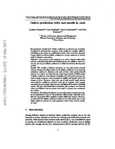
Fig. 2. Principal components extracted from the APP-25, APP-50 and APP-75 datasets.

factors. Unlike other transformations used in PCA, it identifies the most significant code smells collocations, ignoring the smells that are only occasionally related to other smells, which is in line with the objective of this study. The extracted components are presented in Figs. 1–5 along with their eigenvalues, i.e., the amount of explained variance. For each component, we report smells with loading coefficients greater than 0.30. While there are no guidelines recommending this specific value, in this case it provides provides a satisfactory separation of variables with significant and insignificant loadings.

4.2.2. Results for the ALL-* datasets The results obtained for the ALL-* datasets are presented in Fig. 1. The ALL-* datasets include the largest number of projects and contain the largest number of analyzed classes. As a result, almost every code smell is present in one of the datasets, except for the Long Parameter List (absent in the ALL-50 and ALL-75), and Refused Parent Bequest (absent in the ALL-75) smells. The ALL-* datasets display sufficiently high KMO values (0.666–0.728) and their sphericity is also satisfactory (Bartlett’s test is significant in all cases). Therefore, the datasets are good enough for applying PCA. Six components extracted from the ALL-25 dataset explain 58.548% of variance. In the ALL-50, there are five components that account for 49.773% of variance, whereas five components in the ALL-75 represent 52.574% of variance.

Fig. 1. Principal components extracted from ALL-25, ALL-50 and ALL-75 datasets. 7


B. Walter et al.

below the threshold (0.417). However, based on significant results of sphericity test for all datasets, we consider all of them suitable for applying PCA. From the dataset APP-25 we extracted four components representing 51.144% of variance, from APP-50 – six components with 65.095%, and from APP-75 – five components explaining 58.003% of variance. Not all analyzed smells are present in the APP-* datasets: APP-25 and APP-50 do not include Brain Method and Long Parameter List smells, and Refused Parent Bequest is not present in APP-75. The set {Extensive Coupling, Brain Class, God Class, Long Method} is present in all datasets. Additionally, sets {Feature Envy, -Data Class} and {Tradition Breaker, Refused Parent Bequest} are present in APP-25 and APP-50. Surprisingly, there are cases of opposite signs of loading factors in the same smell pattern, e.g., {Extensive Coupling, God Class} is present in all datasets, but a set {-Extensive Coupling, God Class} is present in the APP-75. In a similar way, {-Data Class, Shotgun Surgery} in APP-50 has its counterpart {Data Class, Shotgun Surgery} in APP-75.

Fig. 3. Principal components extracted from the CSS-25, CSS-50 and CSS-75 datasets.

4.2.4. Results for the CSS-* datasets The results for the CSS-* domain are presented in Fig. 3. The KMO values obtained for CSS-25 and CSS-50 datasets (0.668 and 0.582, respectively) are high enough, but for CSS-75 the value is too low (0.409). Even though the sphericity test produced significant results for all datasets, results for the CSS-75 should be treated cautiously. For the three datasets, six components have been extracted, which represent 64.145%, 61.693% and 69.080% of variance, respectively. Like in other domains, some smells are not present in each dataset: Brain Method was not detected in any set, and Long Parameter List and Refused Parent Bequest are missing in the CSS-75. Again, some sets are present in several CSS-* datasets. These include an already reported set {Extensive Coupling, Brain Class, Long Method}, but also another one, {God Class, Shotgun Surgery, Long Method}. Additionally, {Extensive Coupling, Brain Class, Long Method, God Class, Shotgun Surgery}, {Tradition Breaker, Refused Parent Bequest}, {God Class, Long Parameter List}, and {-Data Class, Intensive Coupling} are found in APP-25 and APP-50. The pattern {Feature Envy, -Data Class}, present also in other domains , was found only in APP-25.

Fig. 4. Principal components extracted from DEV-25, DEV-50 and DEV-75 datasets.

4.2.5. Results for the DEV-* datasets The results for the DEV-* datasets are presented in Fig. 4. The KMO values obtained for these datasets lead to mixed conclusions. For the DEV-25, KMO is sufficiently high (0.600), for DEV-50 it is just below the threshold (0.499), but for DEV-75 the value is very low (0.387). Since Bartlett’s test are significant for all tests, we decided to accept the first two datasets and reject the last one. We present the further analysis for all datasets, but results for DEV-75 are inconclusive. For DEV-25 and DEV-50 six components have been extracted. They represent 63.222% and 60.966% of variance, respectively. In case of the dataset DEV-75, five components account for 59.547% of variance. A set {Extensive Coupling, Brain Class, Long Method} is present in all datasets. Some other patterns, like {Tradition Breaker, Refused Parent Bequest}, {Shotgun Surgery, Intensive Coupling} and {God Class, Long Parameter List}, have been found in DEV-25 and DEV-50. The presence of {Feature Envy, -Data Class} is significant only in DEV25, and {-Data Class, Intensive Coupling} only in the DEV-50 dataset.

Fig. 5. Principal components extracted from DGDV-25, DGDV-50 and DGDV-75 datasets.

As follows from Fig. 1, some collocations of smells are common and recur in several datasets, e.g., {Brain Class, God Class, Long Method} and {Extensive Coupling, Intensive Coupling, Schizophrenic Class}. Some other subsets, e.g., {Brain Method, Schizophrenic Class} and {Tradition Breaker, Refused Parent Bequest} are specific to only some datasets (they are present in ALL-25 and ALL-50, but not in ALL-75).

4.2.6. Results for the DGDV-* datasets Results for the DGDV-* dataset are presented in Fig. 5. All KMO values are satisfactory (from 0.520 for DGDV-75 to 0.746 for DGDV-25), and tests of sphericity are also significant. Datasets are good enough for applying PCA. PCA for DGDV-25 identified five components that account for 57.559% of variance, whereas in case of DGDV-50 and DGDV-75 six components have been extracted, which represent 61.404% and

4.2.3. Results for the APP-* datasets The results for the APP-* domain are presented in Fig. 2. The APP-25 and APP-50 datasets also display satisfactory values of KMO (0.663 and 0.553, respectively), while the value for APP-75 is 8


B. Walter et al.

67.337% of variability, respectively. The {Extensive Coupling, Brain Class, God Class, Long Method} pattern is present in all datasets, and in DGDV-25 and DGDV-50 it includes also a Long Parameter List smell. Moreover, these two datasets also contain {Feature Envy, -Data Class} and {TB, Refused Parent Bequest} sets, while {Feature Envy, Brain Method} seems specific to DGDV-50 and DGDV-75 datasets.

4.3. Mining of association rules 4.3.1. Quality metrics of association rules To evaluate the extracted rules, we used four measures: support, confidence (Agrawal et al., 1996), conviction, and lift (Brin et al., 1997). They are defined as follows: let X and Y be item-sets, X → Y an association rule and T a set of transactions in a dataset. Support supp(X) of X with respect to a dataset T is the proportion of transactions that include the item-set X. Then, confidence conf(X → Y ) = supp(X ∪ Y )/supp(X ), the conviction is defined as 1 − supp(Y ) supp(X ∪ Y ) conv(X → Y ) = 1 − conf(X → Y ) , and lift(X → Y ) = supp(X ) × supp(Y ) . We chose conviction as the primary measure of quality. For rules that involve only binary variables, it is more suitable than confidence and support; additionally, unlike support, it takes into account the direction of the rule (Azevedo and Jorge, 2007). To extract association rules, we used apriori algorithm (Agrawal et al., 1993) implemented in the arules R package (Hahsler et al., 2007). Since the presence of a code smell in a class is rather an infrequent event, we set the support to 0.001 to capture also weaker rules. Although the considered datasets include only classes with code smells, not all the classes are affected by the same code smells, thus leading to a rather sparse dataset. We control the number of extracted rules with the conviction and confidence settings, set to ≥ 1 and ≥ 0.60, respectively. The minimum lift was set to 0. In Fig. 6 we present rules found in the ALL-* datasets, as well as relevant quality metrics. Additionally, we present the order of a rule,

Fig. 7. Overview of the rules in the ALL-25 dataset.

i.e., the number of distinct code smells involved in a rule. As follows from the charts, the rules of orders 2 and 3 appear more relevant (in terms of support) than other rules. For that reason, we focus on rules with a maximum order of 3. For the sake of completeness, in Appendix B we include an overview of all rules extracted from all analyzed datasets. 4.3.2. Dataset ALL-25 In Fig. 7 we present overview of rules from the ALL-25 dataset. The LHS (left-hand side) columns show antecedent, and RHS (right-hand side) – the consequent of an association rule. The circle’s size represent the rule’s conviction value and the circle’s color represent the rule’s lift (darker color indicates higher lift). We found several rules with support in the range [0.003, 0.234] and conviction in the range [1.442, 11.185], that combine following code smells: Feature Envy, Shotgun Surgery, Long Parameter List, Long Method, God Class, and Refused Parent Bequest. Table B.18 presents

Fig. 6. Order of association rules found in ALL-* datasets. 9


B. Walter et al.

Table 8 Rules of ordermax=3 in the ALL-50 dataset. LHS → → → → → → → → → → →

{GC, FE} {LPL, SS} {GC} {GC, SS} {LPL, SS} {GC} {LPL, RPB} {SS, LM} {FE} {LPL, RPB} {LPL, SS}

RHS

Support

Confidence

Lift

Conviction

{LM} {FE} {LM} {FE} {GC} {FE} {GC} {FE} {LM} {FE} {LM}

0.112 0.009 0.153 0.066 0.008 0.139 0.001 0.055 0.213 0.001 0.008

0.803 0.747 0.770 0.712 0.667 0.700 0.643 0.680 0.726 0.643 0.653

2.009 2.547 1.927 2.428 3.351 2.388 3.231 2.322 1.816 2.193 1.635

3.047 2.790 2.612 2.451 2.403 2.356 2.243 2.212 2.189 1.979 1.732

Table 9 Rules of ordermax=3 in the ALL-75 dataset. Fig. 8. Graph of the rules in the ALL-25 dataset.

LHS {FE} {GC}

the rules found in the dataset, ordered by conviction, and Fig. 8 visualises these rules. Significant rules combine only few code smells: God Class, Long Parameter List, Feature Envy, Shotgun Surgery, Long Method, and Refused Parent Bequest. As follows from Fig. 8, a few smells are present in the antecedent in rules having Feature Envy smell as a consequence. There is also another rule involving two collocated code smells, namely Long Parameter List, Shotgun Surgery, that implies the presence of three other smells: God Class, Long Method and Feature Envy (Tables 7–9).

4.3.3. Dataset ALL-50 Fig. 9 shows the overview of the rules present in the ALL-50 dataset. We found rules with support in the range [0.001,0.213] and conviction in the range [1.731,3.047], among the following code smells: Feature Envy, Shotgun Surgery, Long Parameter List, Long Method, God Class, Refused Parent Bequest. Table B.23 presents the complete set of rules found in the dataset, ordered by conviction, and Fig. 10 visualizes these rules in a graph. The strongest rules in ALL-50 have been also found in the ALL-25 dataset. As follows from Fig. 8, the number of rules is lower than in the ALL-25 dataset, and in most cases they have been already extracted. Additionally, we found a new rule: Feature Envy → Long Method.

Table 7 Rules of order

max=3

LHS {GC, LPL} {LPL, SS} {GC, LM} {LPL, RPB} {GC} {RPB, LM} {LPL, LM} {RPB, LM} {SS, LM} {LPL, LM} {LPL, SS} {LPL} {SS, RPB} {SS, LM} {GC} {LPL, SS} {LM} {SS} {RPB}

→ → → → → → → → → → → → → → → → → → →

→ →

RHS

Support

Confidence

Lift

Conviction

{LM} {LM}

0.172 0.109

0.976 0.958

1.219 1.196

8.331 4.727

Fig. 9. Overview of the rules of ordermax=3 in the ALL-50 Dataset.

in the ALL-25 dataset. RHS

Support

Confidence

Lift

Conviction

{FE} {FE} {FE} {GC} {FE} {GC} {FE} {FE} {FE} {GC} {GC} {FE} {GC} {GC} {LM} {LM} {FE} {FE} {FE}

0.062 0.027 0.150 0.004 0.202 0.005 0.044 0.005 0.055 0.038 0.022 0.107 0.003 0.044 0.160 0.020 0.234 0.133 0.011

0.956 0.943 0.941 0.885 0.923 0.857 0.900 0.893 0.879 0.784 0.782 0.830 0.699 0.692 0.731 0.692 0.716 0.699 0.659

1.881 1.854 1.851 4.050 1.816 3.921 1.770 1.756 1.728 3.585 3.576 1.632 3.196 3.165 2.232 2.113 1.408 1.374 1.297

11.185 8.555 8.361 6.809 6.384 5.470 4.910 4.589 4.051 3.613 3.578 2.886 2.593 2.536 2.500 2.183 1.728 1.632 1.443

Fig. 10. Graph of the rules in the ALL-50 Dataset.

4.3.4. Dataset ALL-75 Fig. 11 shows the graph of rules in the ALL-75 dataset. We found a number of rules with support in the range [0.109,0.172] and conviction in the range [4.727,8.331], among the following code smells: Feature Envy, Long Method, God Class. Table B.28 and Fig. 11 present the only 10


B. Walter et al.

in a principal component with the loading of the same sign, while (-) denotes a negative correlation or inverse loadings in the component. The presence of smells in a significant associative rule is marked with a plus, if conv ≥ 2.0. A space indicates that no interesting relationship between the smells exists. In Table 13 we report the number of quality dimensions shared among all the smell pairs, according to the metrics part of the detection rule. We consider two smells as related to the same quality dimension, if the detection rules share at least one metrics that belong to that dimension. Correlation analysis identified candidate smells that frequently occur together. For example, various relationships among Brain Class, God Class, Extensive Coupling, and Long Method smells have been identified in all analyzed domains. According to the data reported in Table 13, Brain Class and God Class are expected to be collocated, because they both measure three quality dimensions, namely Size, Complexity and Cohesion. Also Long Method is expected to be collocated with them, because methods affected with the smell frequently belong to Brain Classes or a God Classes. However, Extensive Coupling is rather unexpected in the group: although it also measures Complexity, it does not share any metric with the remaining smells. Additionally, the smells have been found to be related with Long Parameter List in all domains except for CSS, even though it does not share any metric with the other mentioned smells. Long Parameter List may suggest increased coupling of the affected class with the referenced classes. Also two other pairs of smells, {Tradition Breaker, Refused Parent Bequest}, and {Feature Envy, -Data Class} are prevalent. Sometimes, they are accompanied also by God Class or Shotgun Surgery. Tradition Breaker and Refused Parent Bequest manifest an improper use of inheritance and are expected to be related, given that they share two software qualities of interest: Size and Complexity. Similarly, a class affected by Feature Envy references other classes in order to use their methods; conversely, Data Class describes objects used by other classes, so the mutually excluding nature of these smells is justified. Other inter-smell correlations are significant only in selected domains or datasets. Noticeably, the relationships extracted with associative rules do not fully match the results of correlation analysis and PCA. The most significant rules combine few code smells: God Class, Long Parameter List, Feature Envy, Shotgun Surgery, Long Method, and Refused Parent Bequest. Unlike the correlation analysis, the extracted rules do not involve Brain Class, Schizophrenic Class, Intensive Coupling, Tradition Breaker and Extensive Coupling. On the other hand, some new relationships have been identified: Feature Envy → Long Method, Feature Envy → Shotgun Surgery, and God Class → Refused Parent Bequest. All these relationships, except the last one, are not expected according to the data reported in Table 13. There is one more rule involving two collocated code smells, namely {Long Parameter List, Shotgun Surgery}, that implies the presence of three other smells: God Class, Long Method and Feature Envy.

Fig. 11. Graph of the rules in the ALL-75 dataset.

two rules found in the dataset. 4.3.5. Datasets CSS-*, DEV-*, APP-*, and DGDV-* The same analysis was conducted for the CSS-*, DEV-*, APP-*, and DGDV-* datasets. There are not many differences among the domains, so we report only the most relevant ones. As for the ALL-* datasets, the rules of order two and three have the highest support. We report further in this section the results with ordermax=3. In Fig. 12 we present the rules obtained for the CSS-25, DEV-25, APP-25, and DGDV-25 datasets. The most relevant differences among domains are as follows: (a) the presence of the God Class → Long Method rule only in the CSS-25 (support: 0.115, conviction: 1.839) and APP-25 (support: 0.133, conviction: 2.600) datasets, (b) the rule {Refused Parent Bequest,Long Method} → God Class present only in the DEV-25 (support: 0.007, conviction: 9.035) dataset and (c) the Data Class code smell that appears in a rule in the APP-25 dataset: {Data Class, Shotgun Surgery} → Long Method (support: 0.0139, conviction: 1.524). The rules found in the CSS-50, and DEV-50 datasets involve the same smells as in ALL-75 dataset: Feature Envy, Long Method, God Class. The rules found in the APP-50 also see the presence of the Shotgun Surgery code smell, and the rules for DGDV-50 involve both the presence of Shotgun Surgery and Data Class, as reported in Tables 10 and 11, respectively. There is also a difference compared to APP-25 and DGDV-25: for datasets *-50 the presence of Data Class is more evident for the DGDV-50 than for the APP-50 dataset. Among the CSS-75, DEV-75, APP-75, and DGDV-75 datasets, we found two significant rules in CSS-75: Feature Envy → Long Method (support:0.250, conviction: 15.077) and God Class → Long Method (support: 0.144, conviction: 4.588), one significant rule in DEV-75: Feature Envy → Long Method (support: 0.157, conviction: 3.224), one significant rule in APP-75: God Class → Feature Envy (support: 0.060, conviction: 2.161). In DGDV-75 we found the same rules as in other datasets except for God Class → Feature Envy. In addition, we found two rules involving Shotgun Surgery: {Shotgun Surgery, Long Method} → God Class (support: 0.042, conviction: 6.401) and Shotgun Surgery → God Class (support: 0.074, conviction: 4.030).

5.2. RQ2: comparison with Literature As we mentioned in Section 2.4, several relationships reported in literature are only conjectured or do not have adequate empirical support. The co-existence of God Class and Long Method8 has been already reported by Lanza and Marinescu (2005). We expanded the set of closely related smells to God Class, Brain Class, Extensive Coupling, and Long Method. Out of them, the relationship between God Class and Brain Class deserves a comment: although they are defined as disjoint, their detection strategies allow for an overlap of symptoms (Lanza and

5. Discussion of results 5.1. RQ1: summary of code smells collocation results In Table 12 we summarize results of the three procedures in all analyzed working datasets (given in columns): *-25, *-50 and *-75. Significant relationships among smells are marked by respective signs: (+) denotes a positive correlation (∣ρ∣ ≥ 0.3) of smells or their presence

8

11

Named Brain Method, but the definition is equivalent to Long Method.


B. Walter et al.

Fig. 12. Rules of ordermax=3 found in CSS-25, DEV-25, APP-25, and DGDV-25 datasets.

Marinescu, 2005). Our findings show that classes are affected by both smells quite frequently. Since Tradition Breaker appears to be a special case of the Refused Parent Bequest, their co-existence has been also already conjectured (Lanza and Marinescu, 2005). We also confirmed the relationship between Feature Envy and God Class, previously reported in several studies (Lanza and Marinescu, 2005; Lozano et al., 2015; Walter and Pietrzak, 2005; Yamashita and Moonen, 2013a; Yamashita et al., 2015), and that Feature Envy and Data Class are disjoint (Yamashita et al., 2015; Lanza and Marinescu, 2005). The extracted relationship {Feature Envy, -Data Class} corroborates the results reported by Walter and Pietrzak (2005) and Yamashita et al. (2015). In our previous study, we examined the same software systems with respect to correlations between code smells and quality metrics (Arcelli Fontana et al., 2013). Intuitively, smells that are correlated with the same metrics can be also related to each other. Specifically, Brain Class, God Class and Brain Method, strongly correlated with the CYCLO and WMC metrics, are also frequently collocated. Even though their detection strategies do not directly rely on these metrics,

Table 10 Rules including Shotgun Surgery of ordermax=3 in the APP-50 dataset. LHS {GC} {SS, RPB} {LPL, SS} {LPL, SS}

→ → → →

RHS

Support

Confidence

Lift

Conviction

{SS} {FE} {FE} {LM}

0.101 0.004 0.004 0.004

0.633 0.667 0.667 0.667

1.294 2.638 2.638 1.801

1.393 2.242 2.242 1.890

Table 11 Rules including Shotgun Surgery and Data Class smells of ordermax=3 in the DGDV-50 dataset. LHS {FE} {GC} {LPL, RPB} {DC, LM}

→ → → →

RHS

Support

Confidence

Lift

Conviction

{SS} {SS} {SS} {SS}

0.215 0.182 0.007 0.001

0.682 0.665 0.625 1.000

1.208 1.177 1.107 1.771

1.369 1.299 1.161 N/A

12


B. Walter et al.

Table 12 Comparison of significant inter-smell relationships extracted with various procedures. PCA

Correlation

all BC, LM BC, GC BC, EC EC, GC EC, LM EC, SS GC, LM GC, LPL EC, SC GC, SS LM, LPL LM, SS IC, SC FE, GC FE, LM DC, FE RPB, TB FE, LPL FE, SS GC, RPB FE, RPB

+ + + + + + + + + + + + + + + +

app ++ ++ + + + ++

+ + + + + + +

++ +

+++

++

+

+ + + + + + +

css + + + + + +

++ + + + -++

+ + + + + + + + + + + -+ + +

++ + ++ + ++ + + + ++ + ++ + + +

dev

dgdv

+ + + + + + + + + + + + + + +

+ + + + + + + +

++ ++ ++ + ++ + + + ++ -+ +

+ + + + +

+ + + + +

++

all

app

css

dev

dgdv

all

app

css

dev

dgdv

+++ ++

+ + + + + + +

++

++

+++ + + ++ +

+++ + + + + + -

+ + + + + + + +

+++ ++

++ +

+++ ++

++ ++

+++ ++

++ ++ +

++ ++ ++

++ + +

+ + +

+++ ++ ++

++ +++

+++ ++

++ +++

++ ++

++ +++

+ + + +

+ + + +

++ ++ +

++ ++ ++ +

+ + + +

++

+ + ++ + +

++ ++ + -

+ + ++

-++

+

Associative rules

-

-

LM BM LPL GC BC TB EC IC FE SS DC SG RPB SC

BM

LPL

GC

2 0 1 1 0 0 0 0 1 0 0 0

0 1 1 0 1 1 0 1 0 0 0

0 0 0 0 0 0 0 0 0 0

3 1 0 0 1 0 1 1 1

BC

TB

EC

IC

FE

SS

DC

SG

RPB

++

+ ++ + -

++ + + + +

+ + + +

+ + + +

The second column provides a citation if the pair was reported in, otherwise it reports a new finding. We also indicate expected collocations, where the involved smells share at least one quality dimension (according to Table 13). Moreover, in the third column we report the analytic procedure used to discover the finding.

Table 13 Number of shared software quality dimensions included in the code smell detection rule. LM

-

++ + ++ + ++

SC

5.3. RQ3: differences among domains 1 0 0 0 0 1 1 1

0 0 0 0 1 2 1

2 0 0 0 0 0

0 0 0 0 0

0 0 0 0

0 0 0

1 1

-

1

The extracted relationships among code smells are similar, but not identical with respect to the software domain. Three extracted rules indicate differences among domains. They are: (a) God Class → Long Method, present only in the CSS-25 and APP-25 datasets, (b) {Refused Parent Bequest, Long Method} → God Class, present only in the DEV-25 dataset, and (c) {Data Class, Shotgun Surgery} → Long Method only in the APP-25 dataset. The (a) rule confirms that the number of God Class and Long Method instances is highest in the CSS, as reported in Arcelli Fontana et al. (2013). The (b) rule states that classes in DEV domain are more likely to be large and complex, not to use inherited properties and methods, and to have long methods. The (c) rule states that APP classes that store data are frequently called by other classes and expose long methods.

-

they capture complexity of classes. On the other hand, we found Data Class and Feature Envy negatively correlated, whereas their relationship with metrics may lead to an opposite conclusion. Pietrzak and Walter (2006) identified different types of dependencies among smells. The associative rules extracted in this study provide empirical evidence for two of the types: aggregate support and transitive support. For example, in ALL-25 dataset, a rule {God Class, Long Parameter List} → Feature Envy, (conv: 11.185), is stronger than individual rules God Class → Feature Envy (conv: 6.384) and Long Parameter List → Feature Envy (conv: 2.886). Another set of rules illustrates the transitive support: in dataset ALL-25, two simple support relationships have been extracted: God Class → Long Method (conv: 2.500) and Long Method → Feature Envy (conv: 1.728). They both reinforce another rule, God Class → Feature Envy, which is characterized by stronger conviction (6.384) than the source rules individually. These examples show how the relationships among smells can help in detecting other smells. Among the strongest correlations found and outlined in Table 12, we can observe that several correlations mentioned in this section have been previously outlined in the literature, also if many of them have been identified without any empirical validation, with the exception of the work by Palomba et al. (2017). In Table 14 we summarize the collocations reported in Table 12.

5.4. Other findings: impact of the number of detectors Intuitively, the use of a higher number of detectors reduces bias and improves reliability of the smell detection process. On the other hand, it also narrows down the number of detected smell instances and the support for identified relationships. It is reflected by the gradually reduced number of extracted rules in datasets *-25, *-50 and *-75. This is the case for some relationships: {Feature Envy, -Data Class}, {Shotgun Surgery, Intensive Coupling}, and {Shotgun Surgery, Extensive Coupling} are specific to *-25 datasets, and {Tradition Breaker, Refused Parent Bequest} to *-25 and *-50 datasets. It should be noted that the patterns absent in *-75 datasets are still valid, and that relevant collocations of smells could be retrieved even with fewer detectors. In most cases, rules at higher reliability levels have been extracted also by a lower number of detectors. This results from adopting conviction as a quality metric: search for relationships that are both frequent and accurate in smaller datasets results in a lower number of relevant rules. However, some relationships become significant only at higher 13


B. Walter et al.

Table 14 Comparison between our finding and previous ones of the literature. Collocation

Citation/status

Procedure

BC, LM BC, GC BC, EC EC, GC EC, LM EC, SS GC, LM GC, LPL EC, SC GC, SS LM, LPL LM, SS IC, SC FE, GC FE, LM DC, FE RPB, TB FE, LPL FE, SS GC, RPB

Lanza and Marinescu (2005) between GC and Brain Method Expected New Finding Lanza and Marinescu (2005) Lanza and Marinescu (2005) Lanza and Marinescu (2005) Lanza and Marinescu (2005) Lanza and Marinescu (2005), Yamashita and Moonen (2013b), Arcelli Fontana et al. (2015a), Liu et al. (2012), Lozano et al. (2015) Walter and Pietrzak (2005) New Finding New Finding Palomba et al. (2017) New Finding New Finding Lanza and Marinescu (2005), Walter and Pietrzak (2005). Lozano et al. (2015), Liu et al. (2012), Yamashita et al. (2015) Palomba et al. (2017), Lozano et al. (2015) Walter and Pietrzak (2005), Yamashita and Moonen (2013b) Lanza and Marinescu (2005) New Finding New Finding Expected New Finding

PCA, Correlation PCA, Correlation PCA PCA PCA PCA, Correlation PCA, Assoc. rules Assoc. rules PCA PCA, Assoc. rules PCA, Assoc. rules PCA, Assoc. rules PCA, Assoc. rules Assoc. rules Assoc. Rules PCA PCA Assoc. Rules Assoc. Rules Assoc. Rules

reliability levels, e.g., Feature Envy → Long Method rule was identified only in the *-50 and *75 datasets, and a set {-Data Class, Intensive Coupling} is present only at the *-50 level. Also, the relationship {Long Parameter List, Feature Envy} was found in three domains, but mostly in the *-50 datasets, and a set {Schizophrenic Class, -Intensive Coupling} is found only in the *-75 datasets. However, an opposite relationship {Schizophrenic Class, Intensive Coupling} was found in APP-75. This could be an effect of obscuring other smells relevant at lower reliability levels, that became less significant at higher levels

Another example is found in APP-75, where two principal components included contradictory relationships {Schizophrenic Class, -Intensive Coupling} and {Schizophrenic Class, Intensive Coupling}. The positive relationship {Shotgun Surgery with Intensive Coupling} is easy to explain, based on the definitions of smells. Shotgun Surgery refers to a large number of incoming and outgoing calls of an affected method, which is also strongly related to the definitions of Intensive Coupling (a heavy dependency on a number of methods of another classes). The discrepancies between correlation analysis and PCA could be attributed to differences in the techniques. High correlation explicitly indicates that two smells are frequently collocated in same classes. On the other hand, smells present in a single component extracted with PCA, share more abstract factors, and do not have to be actually collocated. For example, only some smells present in the component {EC, BC, GC, SS, LPL, LM} are actually strongly correlated: it is the case for {BC, GC} and {BC, LM}, but no smell is significantly correlated with Shotgun Surgery or Long Parameter List, although they also belong to the component. As a result, PCA performs well in identifying candidate collocations of several smells exhibiting similar properties, while correlation delivers a quantitative measure of the relationship among two smells. Noticeably, extracted associative rules identify a largely disjoint set of relationships than PCA and correlation analysis. In this work, the relevance of associative rules is evaluated by conviction, which is a combination of support and confidence. As a result, rules that are simultaneously frequent and accurate are preferred to ones that are strong, but not very common, which are frequently identified with PCA and correlation analysis. Therefore, the use of diverse procedures provides a more complete perspective of the inter-smell relationships.

5.5. Other findings: differences among procedures There are differences in extracted relationships depending on the procedure used for analysis. Results of correlation analysis and PCA are partially similar, since the correlation analysis is one of first steps in PCA. However, there are also some differences. In general, correlation analysis reveals fewer collocations of smells than PCA, both with respect to the number of extracted pairs of smells and among datasets, in which the pair was identified. For example, {God Class, Shotgun Surgery} or {Long Method, Shotgun Surgery}, extracted in most datasets by PCA, have been identified by the correlation analysis only in a single working dataset. That could suggest differences in thresholds adopted for both techniques; however, other relationships, e.g., {BrainClass, ExtensiveCoupling}, have been extracted by both methods in the same datasets. Moreover, a negatively correlated pair {Intensive Coupling, Schizophrenic Class} was found only in DEV and DGDV domains by correlation analysis, while PCA produced components including these smells in all domains. The same happened to associations {God Class, Shotgun Surgery}, {Long Method, Long Parameter List}, and {Long Method, Shotgun Surgery}, which were highly correlated only in DGDV domain, although they were identified in extracted principal components in all domains. Conversely, a pattern {Intensive Coupling, -Data Class} was found in all domains, but it has not been identified (in any domain) by analyzing correlations. In two cases, relationships identified in different domains are contradictory. As depicted in Fig. 2, in the dataset APP-50, PCA identified a {-Data Class, Intensive Coupling, Shotgun Surgery} coupling, while in APP-75 it found a {Data Class, Shotgun Surgery} pair. The opposite signs at the Data Class are particularly interesting, as they happen in the same domain. That indicates significant differences in detecting capabilities of different tools, referring to either of the involved smells.

6. Threats to validity 6.1. Construct validity Discussing relationships among code smells we can refer to various meaning of the term. In this work, we consider smells as related if they affect a single class at the same time. Some smells are related to methods, whereas other are attributed to a class. In our study, the granularity was adjusted to the class-level, which could relate smells found in two methods in the same class. Therefore, analysis of methodand class-level smells in the same classes could lead to wrong conclusions. 14


B. Walter et al.

Additionally, the term “relationship“ could also refer to other types of links between smells, e.g., their temporal or casual dependency, where one smell facilitates introduction or removal of another smell. These relationships are not considered in this work.

the research questions formulated in Section 1. RQ1 concerned the identification of relationships of smells. We extracted a number of various collocations, using three analytic procedures, in fifteen different datasets. The results show that some collocations are more frequent than other. There are also differences with respect to the number of detectors used for smell identification. To a minor extent some of them also depend on the software domain. Looking for an answer to RQ2, we experimentally verified existence of several relationships conjectured in other studies. Since a large share of these studies were not empirically supported, our work provides an experimental evidence for them. Some of the results questioned the previously proposed relationships or identified a few collocations that have not been reported before. We also analyzed if the extracted relationships depend on the domain of software systems (RQ3). The results indicated that a software domain insignificantly affect inter-smell relationships and their relevance; despite of that, we notice some differences among domains. Additionally, we found that identified relationships depend on the method used for extraction. Methods based on correlation analysis and mining associative rules seems complementary, which indicates their equal importance for analysis of code smells. Research presented in this study could be extended in a number of directions. First, there is a need for experimental comparison of code smell detection tools and approaches with respect to their capabilities and accuracy. That could help in choosing a diverse toolbox, adjusted to a given context, which could serve as a reference for smell detection. In future, a new meta-detector, based on specialized detectors, could use the knowledge apply contextual strategies for smell detecting. Further, the results could lead to developing a benchmark for detectors. To foster future research we made the data used in this study publicly available. The relevance of smell collocations has been already outlined in other studies. These relationships could affect important code properties, e.g., change- and defect-proneness of the affected classes. They could also help improving the accuracy of smell identification and propose customized refactorings to eradicate the smells. It is an open question if the relationships could be effectively used, e.g., to estimating technical debt.

6.2. Internal validity Although we aimed at cross-validating the detected instances of smells, some of the smells (Brain Method, Brain Class, Schizophrenic Class, Tradition Breaker, Speculative Generality, Extensive Coupling, and Intensive Coupling) are specific to a single detector, namely iPlasma. Therefore, the identified relationships that include these code smells should be treated more cautiously. 6.3. External validity The results, although obtained from a large dataset, cannot be freely extrapolated. All analyzed systems have been developed in open source (FLOSS) communities, which could be representative for them, but cannot be claimed to be comparable with commercial development methods. The other issue concerns the analysis of software domains. The definitions of domains are not strict and are derived from the functional properties contained in the projects descriptions in Qualitas Corpus. Other methods of assigning systems to domains is also possible, and could yield different results. 6.4. Conclusion validity The conclusions concerning the identified relationships among code smells and the role of a software domain of the system as a contextual variable are supported by the collected evidence. The main threat about the conclusion validity is related with the bias introduced by the choice of detectors. 7. Conclusions and future work In this paper we presented an empirical study on collocated code smells. Results presented in Section 4 allow for providing responses to Appendix A. Correlation matrixes for code smells

Table A1 Correlation matrix for smells in ALL-25 dataset.

BM EC IC SC SG BC TB GC FE DC LPL SS RPB LM

BM

EC

IC

SC

SG

BC

TB

GC

FE

DC

LPL

SS

RPB

LM

1.000 0.020 −0.001 0.021 0.000 −0.001 0.000 0.013 0.003 −0.002 −0.001 −0.001 0.000 0.013

0.020 1.000 0.193 0.125 0.003 0.287 0.088 0.230 −0.055 −0.078 0.235 0.289 0.122 0.250

−0.001 0.193 1.000 0.076 −0.003 0.062 0.048 0.111 −0.089 −0.082 0.108 0.147 0.049 0.043

0.021 0.125 0.076 1.000 0.004 0.046 0.023 0.115 −0.070 −0.043 0.111 0.057 0.033 0.048

0.000 0.003 −0.003 0.004 1.000 −0.002 0.009 −0.005 −0.036 −0.015 0.000 −0.006 −0.003 −0.007

−0.001 0.287 0.062 0.046 −0.002 1.000 0.037 0.310 0.044 −0.065 0.153 0.141 0.039 0.341

0.000 0.088 0.048 0.023 0.009 0.037 1.000 0.097 −0.003 −0.022 0.091 0.051 0.314 0.059

0.013 0.230 0.111 0.115 − 0 .005 0.310 0.097 1.000 0.155 −0.152 0.253 0.227 0.101 0.399

0.003 −0.055 −0.089 −0.070 −0.036 0.044 −0.003 0.155 1.000 −0.388 0.060 −0.001 −0.007 0.012

−0.002 −0.078 −0.082 −0.043 −0.015 −0.065 −0.022 −0.152 −0.388 1.000 −0.058 −0.062 −0.020 −0.098

−0.001 0.235 0.108 0.111 0.000 0.153 0.091 0.253 0.060 −0.058 1.000 0.135 0.069 0.182

−0.001 0.289 0.147 0.057 −0.006 0.141 0.051 0.227 −0.001 −0.062 0.135 1.000 0.066 0.184

0.000 0.122 0.049 0.033 −0.003 0.039 0.314 0.101 −0.007 −0.020 0.069 0.066 1.000 0.050

0.013 0.250 0.043 0.048 −0.007 0.341 0.059 0.399 0.012 −0.098 0.182 0.184 0.050 1.000

15


B. Walter et al.

Table A2 Correlation matrix for smells confirmed by at least 2 out of 4 of detectors.

BM EC IC SC SG BC TB GC FE DC LPL SS RPB LM

BM

EC

IC

SC

SG

BC

TB

GC

FE

DC

LPL

SS

RPB

LM

1.000 0.020 −0.001 0.021 0.000 −0.001 0.000 0.023 0.013 −0.001 0.000 − 0 .001 0.000 0.019

0.020 1.000 0.193 0.125 0.003 0.287 0.088 0.202 0.110 −0.025 0.155 0.289 0.122 0.270

−0.001 0.193 1.000 0.076 −0.003 0.062 0.048 0.117 0.114 −0.030 0.068 0.147 0.049 0.053

0.021 0.125 0.076 1.000 0.004 0.046 0.023 0.107 0.015 −0.019 0.028 0.057 0.033 0.032

0.000 0.003 −0.003 0.004 1.000 −0.002 0.009 −0.005 −0.007 −0.006 0.005 −0.006 −0.003 0.000

−0.001 0.287 0.062 0.046 −0.002 1.000 0.037 0.356 0.184 −0.024 0.066 0.141 0.039 0.441

0.000 0.088 0.048 0.023 0.009 0.037 1.000 0.092 0.029 −0.008 0.115 0.051 0.314 0.057

0.023 0.202 0.117 0.107 −0.005 0.356 0.092 1.000 0.320 −0.033 0.129 0.215 0.079 0.426

0.013 0.110 0.114 0.015 −0.007 0.184 0.029 0.320 1.000 −0.052 0.085 0.131 0.031 0.318

−0.001 −0.025 −0.030 −0.019 − 0 .006 −0.024 −0.008 −0.033 −0.052 1.000 −0.005 −0.018 −0.002 −0.034

0.000 0.155 0.068 0.028 0.005 0.066 0.115 0.129 0.085 −0.005 1.000 0.081 0.054 0.136

−0.001 0.289 0.147 0.057 −0.006 0.141 0.051 0.215 0.131 −0.018 0.081 1.000 0.066 0.137

0.000 0.122 0.049 0.033 − 0 .003 0.039 0.314 0.079 0.031 −0.002 0.054 0.066 1.000 0.040

0.019 0.270 0.053 0.032 0.000 0.441 0.057 0.426 0.318 −0.034 0.136 0.137 0.040 1.000

Table A3 Correlation matrix for smells confirmed by at least 3 of 4 of detectors (note: LPL and RPB are removed).

BM EC IC SC SG BC TB GC FE DE SS LM

BM

EC

IC

SC

SG

BC

TB

GC

FE

DC

SS

LM

1.000 0.020 −0.001 0.021 0.000 −0.001 0.000 0.054 0.024 0.000 0.000 0.027

0.020 1.000 0.193 0.125 0.003 0.287 0.088 0.173 0.118 −0.017 0.081 0.199

−0.001 0.193 1.000 0.076 −0.003 0.062 0.048 0.092 0.149 −0.013 0.062 0.050

0.021 0.125 0.076 1.000 0.004 0.046 0.023 0.100 0.049 −0.015 0.041 0.033

0.000 0.003 −0.003 0.004 1.000 −0.002 0.009 −0.003 0.001 −0.003 −0.001 −0.004

−0.001 0.287 0.062 0.046 −0.002 1.000 0.037 0.230 0.128 −0.012 0.044 0.510

0.000 0.088 0.048 0.023 0.009 0.037 1.000 0.068 0.024 −0.004 0.092 0.055

0.054 0.173 0.092 0.100 −0.003 0.230 0.068 1.000 0.202 −0.007 0.191 0.259

0.024 0.118 0.149 0.049 0.001 0.128 0.024 0.202 1.000 −0.015 0.052 0.167

0.000 −0.017 −0.0013 −0.015 −0.003 −0.012 −0.004 −0.007 −0.015 1.000 −0.002 −0.013

0.000 0.081 0.062 0.041 −0.001 0.044 0.092 0.191 0.052 −0.002 1.000 0.081

0.027 0.199 0.050 0.033 −0.004 0.510 0.055 0.259 0.167 −0.013 0.081 1.00

Appendix B. Association rules for code smells

Table B1 Rules of ordermax=3 in the ALL-25 dataset. LHS {GC, LPL} {LPL, SS} {GC, LM} {LPL, RPB} {GC} {RPB, LM} {LPL, LM} {RPB, LM} {SS, LM} {LPL, LM} {LPL, SS} {LPL} {SS, RPB} {SS, LM} {GC} {LPL, SS} {LM} {SS} {RPB}

→ → → → → → → → → → → → → → → → → → →

RHS

Support

Confidence

Lift

Conviction

{FE} {FE} {FE} {GC} {FE} {GC} {FE} {FE} {FE} {GC} {GC} {FE} {GC} {GC} {LM} {LM} {FE} {FE} {FE}

0.062 0.027 0.150 0.004 0.202 0.005 0.044 0.005 0.055 0.038 0.022 0.107 0.003 0.044 0.160 0.020 0.234 0.133 0.011

0.956 0.943 0.941 0.885 0.923 0.857 0.900 0.893 0.879 0.784 0.782 0.830 0.699 0.692 0.731 0.692 0.716 0.699 0.659

1.881 1.854 1.851 4.050 1.816 3.921 1.770 1.756 1.728 3.585 3.576 1.632 3.196 3.165 2.232 2.113 1.408 1.374 1.297

11.185 8.555 8.361 6.809 6.384 5.470 4.910 4.589 4.051 3.613 3.578 2.886 2.593 2.536 2.500 2.183 1.728 1.632 1.443

16


B. Walter et al.

Table B2 Rules of ordermax=3 in the APP-25 dataset. LHS {RPB, LM} {GC, LPL} {GC, LM} {GC, RPB} {GC, DC} {GC} {LPL, SS} {LPL, SS} {LPL, LM} {GC} {LPL, SS} {SS, RPB} {RPB} {RPB} {SS, LM} {LPL} {LM} {DC, SS} {SS}

→ → → → → → → → → → → → → → → → → → →

RHS

Support

Confidence

Lift

Conviction

{GC} {FE} {FE} {FE} {LM} {FE} {FE} {GC} {FE} {LM} {LM} {GC} {GC} {FE} {FE} {FE} {FE} {LM} {FE}

0.005 0.062 0.119 0.006 0.004 0.151 0.027 0.023 0.055 0.133 0.024 0.002 0.007 0.008 0.076 0.129 0.267 0.014 0.139

0.857 0.900 0.896 0.889 0.833 0.867 0.854 0.732 0.837 0.765 0.756 0.667 0.643 0.786 0.780 0.764 0.684 0.600 0.655

4.927 1.748 1.740 1.726 2.135 1.684 1.658 4.206 1.626 1.961 1.937 3.832 3.695 1.526 1.514 1.483 1.329 1.537 1.271

5.782 4.850 4.661 4.365 3.658 3.654 3.314 3.079 2.979 2.600 2.500 2.478 2.313 2.263 2.200 2.052 1.537 1.524 1.404

RHS

Support

Confidence

Lift

Conviction

{FE} {FE} {FE} {FE} {FE} {FE} {GC} {GC} {GC} {FE} {GC} {GC} {GC} {LM} {FE} {SS} {LM} {FE} {FE} {FE}

0.086 0.044 0.106 0.077 0.056 0.164 0.036 0.049 0.002 0.146 0.063 0.005 0.005 0.033 0.005 0.004 0.115 0.013 0.149 0.013

0.964 0.955 0.923 0.901 0.898 0.891 0.780 0.780 0.778 0.843 0.744 0.737 0.722 0.712 0.722 0.611 0.622 0.673 0.633 0.610

2.168 2.146 2.075 2.025 2.019 2.003 4.228 4.224 4.214 1.895 4.030 3.992 3.913 2.335 1.623 2.589 2.040 1.512 1.423 1.372

15.605 12.213 7.239 5.598 5.459 5.103 3.712 3.701 3.669 3.540 3.183 3.099 2.936 2.414 1.998 1.965 1.839 1.696 1.512 1.424

RHS

Support

Confidence

Lift

Conviction

{FE} {FE} {GC} {FE} {FE} {FE} {GC} {FE} {GC} {FE} {GC} {FE} {LM}

0.032 0.080 0.007 0.052 0.007 0.090 0.006 0.126 0.044 0.149 0.026 0.059 0.023

0.957 0.952 0.909 0.910 0.909 0.891 0.842 0.857 0.774 0.835 0.772 0.832 0.685

2.382 2.370 5.088 2.265 2.264 2.218 4.713 2.133 4.333 2.078 4.320 2.073 2.348

13.763 12.457 9.035 6.625 6.582 5.485 5.202 4.178 3.637 3.620 3.598 3.572 2.247

Table B3 Rules of ordermax=3 in the CSS-25 dataset. LHS {GC, LPL} {LPL, SS} {GC, LM} {SS, LM} {LPL, LM} {GC} {LPL, SS} {LPL, LM} {LPL, RPB} {LPL} {SS, LM} {SS, RPB} {RPB, LM} {LPL, SS} {RPB, LM} {RPB, LM} {GC} {DC, SS} {SS} {RPB}

→ → → → → → → → → → → → → → → → → → → →

Table B4 Rules of ordermax=3 in the DEV-25 dataset. LHS {LPL, SS} {GC, LPL} {RPB, LM} {LPL, LM} {RPB, LM} {GC, LM} {LPL, RPB} {LPL} {LPL, LM} {GC} {LPL, SS} {SS, LM} {LPL, SS}

→ → → → → → → → → → → → →

17


B. Walter et al.

Table B5 Rules of ordermax=3 in the DGDV-25 dataset. LHS {RPB, LM} {GC, SS} {LPL, RPB} {LPL, SS} {SS, RPB} {GC, LM} {FE, RPB} {GC} {SS, RPB} {RPB, LM} {RPB} {LPL, SS} {RPB} {SS, LM} {LPL, LM} {LPL, LM} {LPL} {SS, LM} {SS} {LPL, RPB} {SS, RPB} {LPL, SS} {GC} {GC} {RPB} {LM}

→ → → → → → → → → → → → → → → → → → → → → → → → → →

RHS

Support

Confidence

Lift

Conviction

{FE} {FE} {GC} {FE} {FE} {FE} {GC} {FE} {GC} {GC} {FE} {GC} {GC} {FE} {GC} {FE} {FE} {GC} {FE} {LM} {LM} {LM} {LM} {LPL} {LM} {FE}

0.021 0.122 0.018 0.073 0.014 0.172 0.030 0.243 0.014 0.019 0.033 0.068 0.030 0.111 0.107 0.117 0.241 0.086 0.202 0.014 0.011 0.054 0.179 0.156 0.021 0.275

0.971 0.970 0.935 0.959 0.958 0.958 0.923 0.953 0.917 0.912 0.945 0.885 0.873 0.912 0.810 0.890 0.853 0.711 0.832 0.742 0.708 0.705 0.703 0.612 0.021 0.729

1.673 1.672 3.668 1.653 1.652 1.651 3.620 1.643 3.595 3.575 1.630 3.471 3.422 1.573 3.174 1.535 1.471 2.789 1.435 1.967 1.878 1.869 1.863 2.170 0.618 1.257

14.273 13.993 11.547 10.243 10.075 10.005 9.685 8.993 8.940 8.443 7.696 6.492 5.853 4.791 3.911 3.833 2.862 2.581 2.506 2.413 2.135 2.111 2.095 1.850 1.639 1.550

RHS

Support

Confidence

Lift

Conviction

{LM} {FE} {LM} {FE} {GC} {FE} {GC} {FE} {LM} {FE} {LM}

0.112 0.009 0.153 0.066 0.008 0.139 0.001 0.055 0.213 0.001 0.008

0.803 0.747 0.770 0.712 0.667 0.700 0.643 0.680 0.726 0.643 0.653

2.009 2.547 1.927 2.428 3.351 2.388 3.231 2.322 1.816 2.193 1.635

3.047 2.790 2.612 2.451 2.403 2.356 2.243 2.212 2.189 1.979 1.732

RHS

Support

Confidence

Lift

Conviction

{GC} {LM} {FE} {GC} {LM} {FE} {FE} {FE} {FE} {LM} {FE} {LM} {SS}

1.007 1.007 1.077 1.004 1.119 1.071 1.109 1.004 1.004 1.004 1.005 1.162 1.101

1.800 1.800 1.754 1.667 1.744 1.690 1.678 1.667 1.667 1.667 1.600 1.641 1.633

1.996 1.162 1.986 1.163 1.011 1.729 1.682 1.638 1.638 1.801 1.375 1.732 1.294

1.199 1.149 1.043 1.520 1.465 1.408 1.319 1.242 1.242 1.890 1.868 1.754 1.393

Table B6 Rules of ordermax=3 in the ALL-50 dataset. LHS {GC, FE} {LPL, SS} {GC} {GC, SS} {LPL, SS} {GC} {LPL, RPB} {SS, LM} {FE} {LPL, RPB} {LPL, SS}

→ → → → → → → → → → →

Table B7 Rules of ordermax=3 in the APP-50 dataset. LHS {RPB, LM} {GC, LPL} {GC, SS} {SS, RPB} {GC} {SS, LM} {GC} {SS, RPB} {LPL, SS} {LPL, SS} {RPB, LM} {FE} {GC}

→ → → → → → → → → → → → →

18


B. Walter et al.

Table B8 Rules of ordermax=3 in the CSS-50 dataset. LHS {LPL, SS} {GC, SS} {GC, FE} {GC, LPL} {LPL, LM} {LPL, LM} {GC} {SS, LM} {LPL, SS} {GC} {RPB, LM} {FE} {GC}

→ → → → → → → → → → → → →

RHS

Support

Confidence

Lift

Conviction

{FE} {FE} {LM} {FE} {FE} {GC} {LM} {FE} {GC} {FE} {FE} {SS} {SS}

0.016 0.095 0.084 0.014 0.014 0.013 0.125 0.085 0.012 0.123 0.005 0.205 0.134

0.810 0.706 0.679 0.682 0.682 0.636 0.662 0.662 0.619 0.652 0.625 0.744 0.711

2.942 2.567 2.575 2.478 2.478 3.372 2.508 2.405 3.280 2.369 2.272 1.183 1.131

3.806 2.468 2.296 2.278 2.278 2.231 2.176 2.143 2.130 2.081 1.933 1.449 1.285

RHS

Support

Confidence

Lift

Conviction

{GC} {GC} {GC} {FE} {LM} {GC} {LM} {FE} {FE} {FE} {SS}

0.008 0.003 0.007 0.056 0.062 0.009 0.093 0.088 0.049 0.006 0.112

0.889 0.750 0.700 0.701 0.706 0.643 0.682 0.644 0.627 0.600 0.628

6.492 5.477 5.112 3.931 2.946 4.695 2.845 3.609 3.512 3.363 1.017

7.768 3.452 2.877 2.750 2.585 2.417 2.390 2.307 2.201 2.054 1.029

RHS

Support

Confidence

Lift

Conviction

{FE} {LM} {GC} {LM} {GC} {LM} {FE} {LM} {GC} {GC} {FE} {FE} {GC} {LM} {LM} {FE} {FE} {GC} {FE} {GC} {LM} {SS} {SS} {SS}

0.010 0.057 0.025 0.067 0.045 0.047 0.045 0.009 0.025 0.100 0.048 0.100 0.026 0.092 0.111 0.023 0.121 0.007 0.083 0.048 0.176 0.215 0.182 0.007

0.875 0.848 0.810 0.807 0.756 0.780 0.756 0.750 0.708 0.704 0.717 0.704 0.667 0.700 0.691 0.667 0.664 0.625 0.633 0.600 0.644 0.682 0.665 0.625

2.770 2.339 2.958 2.227 2.763 2.153 2.394 2.069 2.588 2.573 2.271 2.229 2.436 1.931 1.906 2.111 2.102 2.284 2.005 2.193 1.776 1.208 1.177 1.107

5.473 4.190 3.813 3.304 2.978 2.904 2.805 2.550 2.490 2.455 2.421 2.312 2.179 2.125 2.063 2.052 2.036 1.937 1.866 1.816 1.789 1.369 1.299 1.161

Table B9 Rules of ordermax=3 in the DEV-50 dataset. LHS {FE, LPL} {LPL, RPB} {RPB, LM} {GC, SS} {GC, FE} {FE, RPB} {GC} {GC} {SS, LM} {LPL, SS} {FE}

→ → → → → → → → → → →

Table B10 Rules of ordermax=3 in the DGDV-50 dataset. LHS {LPL, RPB} {GC, LPL} {RPB, LM} {FE, LPL} {LPL, SS} {LPL, SS} {LPL, SS} {LPL, RPB} {SS, RPB} {SS, LM} {GC, LPL} {SS, LM} {FE, RPB} {LPL} {GC, FE} {SS, RPB} {GC, SS} {LPL, RPB} {LPL} {RPB} {GC} {FE} {GC} {LPL, RPB}

→ → → → → → → → → → → → → → → → → → → → → → → →

19


B. Walter et al.

Table B11 Rules of ordermax=3 in the ALL-75 dataset. LHS {FE} {GC}

→ →

RHS

Support

Confidence

Lift

Conviction

{LM} {LM}

0.172 0.109

0.976 0.958

1.219 1.196

8.331 4.727

RHS

Support

Confidence

Lift

Conviction

{FE}

0.060

0.643

2.817

2.161

RHS

Support

Confidence

Lift

Conviction

{LM} {LM}

0.250 0.144

0.978 0.929

1.455 1.381

15.078 4.589

RHS

Support

Confidence

Lift

Conviction

{LM}

0.158

0.929

1.206

3.224

Table B12 Rules of ordermax=3 in the APP-75 dataset. LHS {GC}

→

Table B13 Rules of ordermax=3 in the CSS-75 dataset. LHS {FE} {GC}

→ →

Table B14 Rules of ordermax=3 in the DEV-75 dataset. LHS {FE}

→

Table B15 Rules of ordermax=3 in the DGDV-75 dataset. LHS {SS, LM} {SS} {GC} {FE}

→ → → →

RHS

Support

Confidence

Lift

Conviction

{GC} {GC} {LM} {LM}

0.043 0.075 0.257 0.166

0.889 0.824 0.889 0.886

3.078 2.852 1.123 1.119

6.401 4.030 1.877 1.825

References

Workshop on Refactoring Tools. ACM, pp. 33–36. Azadi, U., Arcelli Fontana, F., Zanoni, M., 2018. Machine learning based code smell detection through wekanose. Proceedings of the 40th International Conference Software Engineering (ICSE 2018). IEEE, Gothenburg, Sweden. Poster track Azevedo, P.J., Jorge, A.M., 2007. Comparing rule measures for predictive association rules. Proceedings of European Conference on Machine Learning (ECML 2007). Springer, pp. 510–517. Bartlett, M.S., 1937. Properties of sufficiency and statistical tests. Proc. R. Soc. Lond. A: Math. Phys. Eng. Sci. 160, 268–282. http://dx.doi.org/10.1098/rspa.1937.0109. http://rspa.royalsocietypublishing.org/content/160/901/268. Brin, S., Motwani, R., Ullman, J.D., Tsur, S., 1997. Dynamic itemset counting and implication rules for market basket data. ACM SIGMOD Record. 26. pp. 255–264. ACM Chatzigeorgiou, A., Manakos, A., 2010. Investigating the evolution of bad smells in object-oriented code. Proceedings of the 2010 Seventh International Conference on the Quality of Information and Communications Technology. IEEE, pp. 106–115. http:// dx.doi.org/10.1109/QUATIC.2010.16. Cohen, J., 1988. Statistical Power Analysis for the Behavioral Sciences, 2nd ed. Routledge. Collins, M., Dasgupta, S., Schapire, R.E., 2001. A generalization of principal component analysis to the exponential family. Proceedings of the 14th International Conference on Neural Information Processing Systems: Natural and Synthetic (NIPS’01). MIT Press, Cambridge, MA, USA, pp. 617–624. http://dl.acm.org/citation.cfm?id= 2980539.2980620. Counsell, S., Hierons, R.M., Hamza, H., Black, S., Durrand, M., 2010. Is a strategy for code smell assessment long overdue? Proceedings of the Workshop on Emerging Trends in Software Metrics. Cramér, H., 1946. Mathematical Methods of Statistics. Princeton Mathematical Series Princeton University Press. https://books.google.pl/books?id=4mkGAQAAIAAJ. Fowler, M., 1999. Refactoring: Improving the Design of Existing Code. Addison-Wesley. Ganesh, S., Sharma, T., Suryanarayana, G., 2013. Towards a principle-based classification of structural design smells. J. Object Technol. 12, 1:1–29. Hahsler, M., Grün, B., Hornik, K., 2007. Introduction to arules–mining association rules and frequent item sets. SIGKDD Explor 2, 1–32. Jancke, S., 2010. Smell Detection in Context. Rheinische Friedrich-Wilhelms-Universität Bonn Diplomarbeit. Kaiser, H.F., 1958. The varimax criterion for analytic rotation in factor analysis.

Abbes, M., Khomh, F., Gueheneuc, Y.G., Antoniol, G., 2011. An empirical study of the impact of two antipatterns, blob and spaghetti code, on program comprehension. Proceedings of the 15th European Conference on Software Maintenance and Reengineering. pp. 181–190. IEEE. doi:10.1109/CSMR.2011.24. Agrawal, R., Imieliński, T., Swami, A., 1993. Mining association rules between sets of items in large databases. ACM SIGMOD Record. 22. ACM, pp. 207–216. Agrawal, R., Mannila, H., Srikant, R., Toivonen, H., Verkamo, A.I., et al., 1996. Fast discovery of association rules. Adv. Knowl. Discov. Data Min. 12, 307–328. Arcelli Fontana, F., Braione, P., Zanoni, M., 2012. Automatic detection of bad smells in code: an experimental assessment. J. Object Technol. 11, 5:1–38. http://dx.doi.org/ 10.5381/jot.2012.11.2.a5. http://www.jot.fm/contents/issue_2012_08/article5. html. Arcelli Fontana, F., Ferme, V., Marino, A., Walter, B., Martenka, P., 2013. Investigating the impact of code smells on system’s quality: an empirical study on systems of different application domains. Proceedings of the 29th IEEE International Conference on Software Maintenance (ICSM 2013). pp. 260–269. http://dx.doi.org/10.1109/ICSM. 2013.37. Arcelli Fontana, F., Ferme, V., Zanoni, M., 2015a. Towards assessing software architecture quality by exploiting code smell relations. Proceedings of IEEE SAM 2015 Workshop, Co-located with ICSE 2015. IEEE, Florence, Italy. Arcelli Fontana, F., Ferme, V., Zanoni, M., Roveda, R., 2015b. Towards a prioritization of code debt: a code smell intensity index. Proceedings of the Seventh International Workshop on Managing Technical Debt (MTD 2015). IEEE, Bremen, Germany. In conjunction with ICSME 2015 Arcelli Fontana, F., Mäntylä, M.V., Zanoni, M., 2015c. Comparing and experimenting machine learning techniques for code smell detection. Empir. Softw. Eng. http://dx. doi.org/10.1007/s10664-015-9378-4. Arcelli Fontana, F., Roveda, R., Zanoni, M., 2016. Technical debt indexes provided by tools: a preliminary discussion. Proceedings of the 8th IEEE International Workshop on Managing Technical Debt, MTD 2016, Raleigh, NC, USA, October 4, 2016. pp. 28–31. https://doi.org/10.1109/MTD.2016.11. Arcoverde, R., Garcia, A., Figueiredo, E., 2011. Understanding the longevity of code smells: preliminary results of an explanatory survey. Proceedings of the 4th

20


B. Walter et al.

repository mining. Proceedings of the 2012 16th European Conference on Software Maintenance and ReEngineering. IEEE, pp. 411–416. http://dx.doi.org/10.1109/ CSMR.2012.79. Pietrzak, B., Walter, B., 2006. Leveraging code smell detection with inter-smell relations. Extreme Programming and Agile Processes in Software Engineering (XP). Springer, Berlin, Heidelberg, pp. 75–84. http://dx.doi.org/10.1007/11499053_18. Rao, A.A., Reddy, K.N., 2008. Detecting bad smells in object oriented design using design change propagation probability matrix. Proceedings of the International MultiConference on Engineers and Computer Scientists. pp. 1001–1007. Ratiu, D., Ducasse, S., Gîrba, T., Marinescu, R., 2004. Using history information to improve design flaws detection. Proceedings of the 8th European Conference on Software Maintenance and Reengineering (CSMR’04). IEEE Computer Society, Washington, DC, USA, pp. 223–232. http://dl.acm.org/citation.cfm?id=977397. 977733. Sjoberg, D.I., Yamashita, A., Anda, B.C., Mockus, A., Dyba, T., 2013. Quantifying the effect of code smells on maintenance effort. IEEE Trans. Softw. Eng. 39, 1144–1156. http://dx.doi.org/10.1109/TSE.2012.89. Tempero, E., Anslow, C., Dietrich, J., Han, T., Li, J., Lumpe, M., Melton, H., Noble, J., 2010. Qualitas corpus: a curated collection of java code for empirical studies. Proceedings of the 2010 Asia Pacific Software Engineering Conference (APSEC2010). pp. 336–345. https://doi.org/10.1109/APSEC.2010.46. Trifu, A., Marinescu, R., 2005. Diagnosing design problems in object oriented systems. Proceedings of the 12th Working Conference on Reverse Engineering (WCRE’05). pp. 10. doi:10.1109/WCRE.2005.15. Tsantalis, N., Chatzigeorgiou, A., 2011. Identification of extract method refactoring opportunities for the decomposition of methods. J. Syst. Softw. 84, 1757–1782. http:// dx.doi.org/10.1016/j.jss.2011.05.016. Viggiato, M., Oliveira, J., Figueiredo, E., 2017. On the Investigation of Domain-sensitive Bad Smells in Information Systems. Walter, B., Pietrzak, B., 2005. Multi-criteria detection of bad smells in code with UTA method. In: Baumeister, H., Marchesi, M., Holcombe, M. (Eds.), Extreme Programming and Agile Processes in Software Engineering (XP). Lecture Notes in Computer Science 3556. Springer, Berlin, Heidelberg, pp. 154–161. http://dx.doi. org/10.1007/b137278. Wettel, R., Lanza, M., 2008. Visually localizing design problems with disharmony maps. Proceedings of the 4th ACM symposium on Software Visuallization (SoftVis ’08). pp. 155. http://dx.doi.org/10.1145/1409720.1409745. http://portal.acm.org/citation. cfm?doid=1409720.1409745. Wieman, R., 2011. Anti-pattern Scanner: An Approach to Detect Anti-patterns and Design Violations. Delft University of Technology Ph.d. thesis tu delft. Yamashita, A., 2013. Assessing the capability of code smells to explain maintenance problems: an empirical study combining quantitative and qualitative data. Empir. Softw. Eng. 19, 1111–1143. http://dx.doi.org/10.1007/s10664-013-9250-3. Yamashita, A., Moonen, L., 2013a. Surveying developer knowledge and interest in code smells through online freelance marketplaces. User Evaluations for Software Engineering Researchers (USER). IEEE. Yamashita, A., Moonen, L., 2013b. To what extent can maintenance problems be predicted by code smell detection? An empirical study. Inf. Softw. Technol. 55, 2223–2242. http://dx.doi.org/10.1016/j.infsof.2013.08.002. Yamashita, A., Zanoni, M., Arcelli Fontana, F., Walter, B., 2015. Inter-smell relations in industrial and open source systems: a replication and comparative analysis. Proceedings of the 31st International Conference on Software Maintenance and Evolution (ICSME2015). IEEE, Bremen, Germany. Yamashita, A.F., Moonen, L., 2013c. Exploring the impact of inter-smell relations on software maintainability: an empirical study. Proceedings of the 35th International Conference on Software Engineering, ICSE ’13, San Francisco, CA, USA, May 18–26, 2013. pp. 682–691. http://dx.doi.org/10.1109/ICSE.2013.6606614. Zhang, M., Hall, T., Baddoo, N., 2011. Code bad smells: a review of current knowledge. J. Softw. Maint. Evol.: Res. Pract. 23, 179–202. http://dx.doi.org/10.1002/smr.521.

Psychometrika 23, 187–200. https://doi.org/10.1007/BF02289233. Kaiser, H.F., 1970. A second generation little jiffy. Psychometrika 35, 401–415. http://dx. doi.org/10.1007/BF02291817. Khomh, F., Di Penta, M., Guéhéneuc, Y.G., Antoniol, G., 2012. An exploratory study of the impact of antipatterns on class change-and fault-proneness. Empir. Softw. Eng. 17, 243–275. Khomh, F., Vaucher, S., Guéhéneuc, Y.G., Sahraoui, H.A., 2009. A bayesian approach for the detection of code and design smells. Proceedings of International COnference on Quality Software. http://dx.doi.org/10.1109/qsic.2009.47. Lanza, M., Marinescu, R., 2005. Object-Oriented Metrics in Practice: Using Software Metrics to Characterize, Evaluate, and Improve the Design of Object-Oriented Systems. Springer Publishing Company, Inc. Li, W., Shatnawi, R., 2007. An empirical study of the bad smells and class error probability in the post-release object-oriented system evolution. J. Syst. Softw. 80, 1120–1128. http://dx.doi.org/10.1016/j.jss.2006.10.018. Liu, H., Ma, Z., Shao, W., Niu, Z., 2012. Schedule of bad smell detection and resolution: a new way to save effort. IEEE Trans, Softw. Eng. 38, 220–235. http://dx.doi.org/10. 1109/TSE.2011.9. Lozano, A., Mens, K., Portugal, J., 2015. Analyzing code evolution to uncover relations. Proceedings of the 2015 IEEE 2nd International Workshop on Patterns Promotion and Anti-patterns Prevention (PPAP). pp. 1–4. http://dx.doi.org/10.1109/PPAP.2015. 7076847. Ma, W., Chen, L., Zhou, Y., Xu, B., Zhou, X., 2015. Are anti-patterns coupled? An empirical study. Proceedings of the 2015 IEEE International Conference on Software Quality, Reliability and Security (QRS),. pp. 242–251. http://dx.doi.org/10.1109/ QRS.2015.43. Maiga, A., Ali, N., Bhattacharya, N., Sabane, A., Guéhéneuc, Y.G., Aimeur, E., 2012. SMURF: a SVM-based incremental anti-pattern detection approach. Proceedings of the 2012 19th Working Conference on Reverse Engineering. pp. 466–475. http://dx. doi.org/10.1109/WCRE.2012.56. http://ieeexplore.ieee.org/lpdocs/epic03/ wrapper.htm?arnumber=6385142. Malhotra, R., 2015. Empirical Research in Software Engineering: Concepts, Analysis, and Applications. Chapman and Hall/CRC. Maneerat, N., Muenchaisri, P., 2011. Bad-smell prediction from software design model using machine learning techniques. Proceedings of the2011 Eighth International Joint Conference on Computer Science and Software Engineering (JCSSE). pp. 331–336. http://ieeexplore.ieee.org/lpdocs/epic03/wrapper.htm?arnumber= 5930143. Mäntylä, M.V., 2005. An experiment on subjective evolvability evaluation of object-oriented software: explaining factors and interrater agreement. Proceedings of the International Conference on Software Engineering. pp. 277–286. http://dx.doi.org/ 10.1109/ISESE.2005.1541837. Mäntylä, M.V., Lassenius, C., 2006. Subjective evaluation of software evolvability using code smells: an empirical study. Empir. Softw. Eng. 11, 395–431. http://dx.doi.org/ 10.1007/s10664-006-9002-8. Mäntylä, M.V., Vanhanen, J., Lassenius, C., 2003. A taxonomy and an initial empirical study of bad smells in code. Proceedings of the IEEE International Conference on Software Maintenance. pp. 381–384. http://dx.doi.org/10.1109/ICSM.2003. 1235447. Mara, L., Honorato, G., Medeiros, F.D., Garcia, A., Lucena, C., 2011. Hist-inspect: A tool for history-sensitive detection of code smells. Proceedings of the Tenth International Conference on Aspect-oriented Software Development Companion (AOSD ’11). ACM, New York, NY, USA, pp. 65–66. http://doi.acm.org/10.1145/1960314.1960335. Marinescu, R., 2005. Measurement and quality in object-oriented design. Proceedings of the IEEE International Conference on Software Maintenance. pp. 701–704. http://dx. doi.org/10.1109/ICSM.2005.63. Martin, R.C., 2008. Clean Code: A Handbook of Agile Software Craftsmanship, 1st ed. Prentice Hall PTR, Upper Saddle River, NJ, USA. McConnell, S., 2004. Code Complete, Second ed. Microsoft Press, Redmond, WA, USA. Moha, N., Guéhéneuc, Y.G., Duchien, L., Le Meur, A.F., 2010. DECOR: a method for the specification and detection of code and design smells. IEEE Trans. Softw. Eng. 36, 20–36. http://dx.doi.org/10.1109/TSE.2009.50. Monden, A., Nakae, D., Kamiya, T., Sato, S., Matsumoto, K., 2002. Software quality analysis by code clones in industrial legacy software. Proceedings of the IEEE Symposium on Software Metrics. pp. 87–94. http://dx.doi.org/10.1109/METRIC. 2002.1011328. Nongpong, K., 2012. Integrating “Code Smells” Detection with Refactoring Tool Support. The University of Wisconsin-Milwaukee Ph.d. thesis. Olbrich, S.M., Cruzes, D.S., Sjøberg, D.I.K., 2010. Are all code smells harmful? A study of god classes and brain classes in the evolution of three open source systems. Proceedings of the IEEE Internatinal Conference on Software Maintenance. pp. 1–10. http://dx.doi.org/10.1109/ICSM.2010.5609564. Palomba, F., Bavota, G., Di Penta, M., Oliveto, R., De Lucia, A., Poshyvanyk, D., 2013. Detecting bad smells in source code using change history information. Proceedings of the 2013 28th IEEE/ACM Internatinal Conference on Automated Software Engineering. IEEE, pp. 268–278. http://dx.doi.org/10.1109/ASE.2013.6693086. Palomba, F., Oliveto, R., Lucia, A.D., 2017. Investigating code smell co-occurrences using association rule learning: a replicated study. Proceedings of the 2017 IEEE Workshop on Machine Learning Techniques for Software Quality Evaluation, MaLTeSQuE@ SANER, Klagenfurt, Austria, February 21, 2017. pp. 8–13. http://dx.doi.org/10. 1109/MALTESQUE.2017.7882010. Pearson, K., 1901. On lines and planes of closest fit to systems of points in space. Philos. Mag. Ser. Series 6. 2, 559–572. http://dx.doi.org/10.1080/14786440109462720. Peters, R., Zaidman, A., 2012. Evaluating the lifespan of code smells using software

Bartosz Walter received Ph.D. in software engineering in 2004, and since then he has been working at Pozna University of Technology, Poland. His main interests include quality of source code, software evolution and maintenance and code smells. As a software engineer, he is also involved in software application projects. Francesca Arcelli Fontana has her degree and Ph.D in Computer Science taken at the University of Milano (Italy). She is currently in the position of Associate Professor at University of Milano Bicocca. The actual research activity principally concerns the software engineering field. In particular software evolution, software quality assessment through machine learning techniques, managing technical debt, design patterns, code smells and architectural smells detection. She is the head of the Software Evolution and Reverse Engineering Lab (http://essere.disco.unimib.it/) at University of Milano Bicocca and she is a Member of the IEEE Computer Society. Vincenzo Ferme is a Ph.D. Candidate at the Software Institute, University of Lugano (USI), Switzerland, supervised by Prof. Cesare Pautasso. His main research focus is on Declarative Performance Engineering in DevOps, and during his Ph.D. he is developing a software for automated end-to-end performance assessment of Web services. Before starting his Ph.D. he was a Software Engineer and Java Developer at Connexun S.r.l. for one year, where he implemented a software system to discover and identify Points Of Interest relevant to cross-cultural communities through data analysis and semantic techniques.

21

Code smells and their collocations_ A large-scale

Code smells and their collocations_ A large-scale

Suggest Documents

Code smells

JSNOSE: Detecting JavaScript Code Smells

Refactoring: Code Smells - Testing Education

Code-smells detection - Google Sites

JSNOSE: Detecting JavaScript Code Smells

Competitive Coevolutionary Code-Smells Detection

On Finding Model Smells Based on Code Smells

Collocations: Pedagogical implications, and their ...

Identification of Refused Bequest Code Smells

Poster: Filtering Code Smells Detection Results - Bicocca

JSNOSE: Detecting JavaScript Code Smells - UBC ECE

Defect prediction with bad smells in code

Context-Based Code Smells Prioritization for Prefactoring

Removing Energy Code Smells with Reengineering Services

Towards a Lean Approach to Reduce Code Smells ...

Towards a Lean Approach to Reduce Code Smells ...

Are Code smells the root cause of faults? A ...

Extending a Taxonomy of Bad Code Smells with ... - Semantic Scholar

Empirical Software Evolvability â Code Smells and ... - Semantic Scholar

The Evolution and Impact of Code Smells - UMD Department of ...

On the evaluation of code smells and detection tools

Table of Esters and Their Smells - James Kennedy - WordPress.com

Lexical Collocations and their Relation to the Online Writing of ...

A LargeScale Gene-Trap Screen for Insertional

Code smells and their collocations_ A large-scale