Hindawi Publishing Corporation e Scientific World Journal Volume 2014, Article ID 146186, 15 pages http://dx.doi.org/10.1155/2014/146186
Research Article Code-Time Diversity for Direct Sequence Spread Spectrum Systems A. Y. Hassan1,2 1 2
Benha Faculty of Engineering, Egypt Faculty of Engineering, Northern Border University, Saudi Arabia
Correspondence should be addressed to A. Y. Hassan;
[email protected] Received 23 January 2014; Accepted 2 March 2014; Published 10 April 2014 Academic Editors: Y. Mao and Z. Zhou Copyright © 2014 A. Y. Hassan. This is an open access article distributed under the Creative Commons Attribution License, which permits unrestricted use, distribution, and reproduction in any medium, provided the original work is properly cited. Time diversity is achieved in direct sequence spread spectrum by receiving different faded delayed copies of the transmitted symbols from different uncorrelated channel paths when the transmission signal bandwidth is greater than the coherence bandwidth of the channel. In this paper, a new time diversity scheme is proposed for spread spectrum systems. It is called code-time diversity. In this new scheme, 𝑁 spreading codes are used to transmit one data symbol over 𝑁 successive symbols interval. The diversity order in the proposed scheme equals to the number of the used spreading codes 𝑁 multiplied by the number of the uncorrelated paths of the channel 𝐿. The paper represents the transmitted signal model. Two demodulators structures will be proposed based on the received signal models from Rayleigh flat and frequency selective fading channels. Probability of error in the proposed diversity scheme is also calculated for the same two fading channels. Finally, simulation results are represented and compared with that of maximal ration combiner (MRC) and multiple-input and multiple-output (MIMO) systems.
1. Introduction Diversity techniques are used when the channel is in a deep fade. If several replicas of the same information signal are transmitted over independent fading channels, the probability that all signal components will fade simultaneously is reduced considerably. There are different ways in which we can provide the receiver with 𝐿 independent fading replicas of the same information signal. Frequency diversity is a diversity method where the information signal is transmitted on 𝐿 carriers. The separation between the successive carriers equals to or exceeds the coherent bandwidth of the channel. Orthogonal frequency division multiplexing (OFDM) transmission is the famous technique that exploits frequency diversity to achieve high data rate and low bit error rate in frequency selective channels [1–3]. OFDM suffers from intercarrier interference (ICI) due to frequency offsets, symbol timing error, and channel estimation errors [4–6]. OFDM systems also suffer from high peak to average power ratio (PAPR) [7, 8].
Another commonly used method for achieving diversity employs multiple antennas. Multiple transmitting antennas are used to transmit the same information signal and multiple receiving antennas are used to receive the independently fading replicas of the transmitted signal through uncorrelated fading paths. A comparative study of space diversity techniques in mobile radio is shown in [9]. Multiple-input and multiple-output (MIMO) system is a well-known system that exploits the antenna diversity to enhance the bit error rate and the channel capacity in fading environments [10, 11]. Time diversity is another diversity method where 𝐿 independent fading version of the same information signal is achieved by transmitting the signal in 𝐿 different time slots. The separation between the successive time slots equals to or exceeds the coherence time of the channel. Time diversity is used in modern communication system through interleaving of the transmitted symbols and through the using of channel codes [12–14]. Some systems use a combination of more than one diversity technique to enhance their performance in fading
2
The Scientific World Journal 0
Ts C1 d1
2Ts C1 d2 C2 d1
3Ts
5Ts
4Ts
C1 d3
C1 d4
C1 d5
···
C2 d2
C2 d3
C2 d4
···
C3 d2
C3 d3
···
C3 d1
Figure 1: The code-time diversity system with 3 orthogonal spreading codes.
channels such as space-time (ST) coding in MIMO systems [15, 16], which use the time and space diversities through encoding the transmitted symbols using space time codes and transmitting the encoded symbols by different antennas in the transmitter. This technique allows the data symbol to be transmitted more than one time through different symbol period and it arrives at the receiver’s antennas through different spatial paths. MIMO-OFDM system is another example of multidiversity system where time, frequency, and space diversities are used to enhance the performance of the data transmission over wireless faded channels [17–20]. In MIMO-OFDM system, the symbols are encoded by using space-time-frequency (STF) block codes. The encoded symbol is transmitted more than once over different periods and carrier frequencies using different transmitting antennas. The uncorrelated fading gains that come from the uncorrelated spatial paths, the different transmitting time slots, and the different transmitting carrier achieve the diversity gain at the receiver. This system has large diversity gain and better performance than space-time coded MIMO systems. The systems that use space diversity such as MIMO systems have the disadvantage of using more than one antenna at the transmitter and the receiver. Multiple antennas need multiple RF drivers (power amplifier at the transmitter and low noise amplifier at the receiver) and this complicates the transmitter and the receiver structure. The spacing between the antennas should be large enough to have uncorrelated fading paths and to reduce the cross correlation and interference between the antennas. The MIMO systems consume more power than single-input and single-output (SISO) systems and they have short lifetime batteries for mobile units. Powerful DSP unit is required for MIMO transceivers because ST and STF encoder and decoder need complex computations. In this paper, we propose a new diversity technique for SISO spread spectrum systems that can achieve a diversity gain like that of the MIMO system but with a single transmitting antenna and a single receiving antenna. The MIMO system has diversity gain with two degrees of freedom (the number of the transmitting and receiving antennas). The proposed diversity scheme has a diversity gain with two degrees of freedom too. Although the proposed system has a single transmitting antenna and a single receiver antenna, the using of 𝑁 spreading codes and 𝐿 uncorrelated propagation paths achieves the diversity gain. Section 2 discusses the idea of code-time diversity in detail. In Section 3 the signal model and the new transmit diversity scheme are represented. The receiver structure of the proposed system is shown in Section 4 with the calculations of the probability of error in
the received data. Section 5 shows the simulation results and some implementation issues.
2. Code-Time Diversity In space-time MIMO system, the encoded data symbol is transmitted more than one time through different symbol periods using different transmitting antennas. The transmission of the symbols through independent time slots lets the received symbol to have independent fading gains. The probability of receiving the transmitted symbol with faded gains through the successive time slots is reduced significantly. Also the usage of different antennas allows the transmitted symbol to have independent propagation paths from the transmitter to the receiver and to have independent fading gain through each path. So they are the different time slots and propagation paths that play the main role in the diversity gain enhancement of the time-space MIMO system. In the proposed code-time diversity technique, we use the same concept of time and space diversities but through another procedure. During each symbol period, the current data symbol and the previous (𝑁 − 1) ones are dispersed in frequency using 𝑁 independent spreading codes sequences for each data symbol. The used spreading codes are taken from a set of 𝑁 orthogonal codes. The dispersed symbols are added together and transmitted using a single antenna. The orthogonality between the used spreading sequences prevents the interference among the transmitted symbols. The same procedure is repeated for each symbol period so that each symbol can be transmitted 𝑁 times through 𝑁 successive symbol periods using, each time, a different spreading code from the set of 𝑁 orthogonal codes. Figure 1 shows an example of how the modulated data symbols are transmitted three times at three successive symbol periods using three different orthogonal spreading codes. By this way, time diversity is achieved and the probability of having 𝑁 faded gains during 𝑁 successive symbols periods is reduced considerably. The space diversity is achieved by controlling the bandwidth of the dispersed symbols to be greater than the coherent bandwidth of the used wireless channel. This allows uncorrelated multipath propagation from the transmitter to the receiver. The using of direct sequence spread spectrum (DSSS) increases the information message bandwidth by a factor equal to the process gain of the spreading process, which is equivalent to the ratio between the data symbol period and the spreading code chip period. By controlling the process gain, the bandwidth of the spread signal can be equal
The Scientific World Journal dk
3
Ts
Ts c1 (t)
c0 (t)
Ts
···
Ts
c2 (t)
cN−1 (t)
s(t)
Figure 2: The code-time diversity DSSS modulator.
to multiples of the coherent bandwidth of the channel. The number of the uncorrelated paths that can be appeared from the transmitter to the receiver is given by Bandwidth of DSSS signal + 0.5⌋ . 𝐿=⌊ Channel coherent bandwidth
𝑁 is the number of the used orthogonal spreading codes. Equation (2) shows the 𝑘th symbol transmission: 𝑁−1
𝑠𝑘 (𝑡) = ∑ 𝑑𝑘−𝑛 𝑐𝑛 (𝑡 − 𝑘𝑇𝑠) , (1)
By the same way, the probability of having spatial faded gains through the uncorrelated propagation paths 𝐿 is reduced significantly. The proposed code-time diversity system has a diversity gain with two degrees of freedoms as the space-time MIMO system. Although the diversity gain in the time-space MIMO system is depending on the number of the antennas in the transmitter 𝑁𝑡 and the receiver 𝑁𝑟 , the diversity gain in the code-time diversity system is depending on the number of the used spreading codes 𝑁 (which equals to the number of time slots through which each symbol will be repeated) and the number of the uncorrelated propagation paths 𝐿. The proposed diversity scheme uses one antenna and one RF interface unit in the transmitter and in the receiver. However, the code-time diversity seems to have diversity gain similar to that of the time-space MIMO system, and the code-time diversity uses a spread signal with higher bandwidth than the bandwidth of the transmitted signal in the time-space MIMO system. In other words, the increase in the signal bandwidth of the proposed code-time diversity system is the cost that should be paid to improve the diversity gain using a simplified hardware of single antenna and single RF interface in the transmitter and in the receiver. The code-time diversity system needs no space-time codes, and it depends only on the orthogonality between the spreading codes.
3. Transmitted Signal Model of Code-Time Diversity DSSS The code-time diversity system is based on the transmission of the data by using different orthogonal spreading codes at different transmission periods. At each transmission period, the transmitted signal is the summation between the current spread symbol and the previous (𝑁−1) spread symbols where
(2)
𝑛=0
where 𝑑𝑘−𝑛 is the modulated data symbol and 𝑐𝑛 (𝑡) is the spreading code sequence. The used modulation method may be BPSK or 𝑀-QAM. The spreading codes are assumed to be orthonormal through the symbol period 𝑇𝑠 : 𝑇𝑠 1 ∫ 𝑐𝑖 (𝑡) ⋅ 𝑐𝑗 (𝑡) ⋅ 𝑑𝑡 = { 0 0
if 𝑖 = 𝑗 if 𝑖 ≠ 𝑗.
(3)
Without any loss of generality, the code period is assumed to be equal to the symbol period: 𝑇𝑠 = 𝑁𝑐 ∗ 𝑇𝑐 .
(4)
𝑁𝑐 is the number of chips on one code period and 𝑇𝑐 is the chip period. So, 𝑐𝑖 (𝑡 − 𝑘𝑇𝑠 ) = 𝑐𝑖 (𝑡) .
(5)
The transmitted signal of a packet of 𝐾 symbols is illustrated in (6) and Figure 2 shows the modulator structure of codetime diversity system: 𝐾−1
𝐾−1 𝑁−1
𝑘=0
𝑘=0 𝑛=0
𝑠 (𝑡) = ∑ 𝑠𝑘 (𝑡 − 𝑘𝑇𝑠) = ∑ ∑ 𝑑𝑘−𝑛 𝑐𝑛 (𝑡 − 𝑘𝑇𝑠) .
(6)
The modulated signal in (6) is transmitted to the channel through single RF interface module and single transmitting antenna.
4. Received Signal Model of Code-Time Diversity DSSS Signal in Rayleigh Fading Channel and the Proposed Demodulator Building 4.1. Flat Fading Rayleigh Channel. The impulse response of the flat fading channel is shown in (7). Quasistatic channel is
4
The Scientific World Journal
assumed where the fading gain is fixed during one symbol period and it is changed randomly from one symbol to another: ℎ (𝑡) = 𝛼𝛿 (𝑡) ,
(7)
where 𝛼 is a complex Gaussian random variable with zero mean and 𝜎𝛼2 variance. In flat fading channel, the transmitted signal travels from the transmitter to the received through unresolvable propagation paths. Therefore, all frequency components of the signal will experience the same magnitude of fading. In our proposed diversity scheme, the flat fading case looks like the MISO system where multiple antennas transmit the modulated symbols and a single antenna at the receiver picks them up. According to our signal model, the received signal at the demodulator input is 𝐾−1 𝑁−1
𝑟 (𝑡) = ∑ ∑ 𝛼𝑘 𝑑𝑘−𝑛 𝑐𝑛 (𝑡 − 𝑘𝑇𝑠) + 𝑤 (𝑡) ,
(8)
𝑘=0 𝑛=0
where 𝑤(𝑡) is a sample function of white Gaussian noise process with zero mean and 𝜎𝑤2 variance. 𝛼𝑘 is the channel random gain at the 𝑘th symbol period. The proposed demodulator for the code-time diversity system consists of three parts. The first part is a bank of correlators that correlate the received signal with the 𝑁 spreading codes. The 𝑛th correlator correlates the received signal with the 𝑛th spreading code 𝑐𝑛 (𝑡) through one symbol period. The 𝑛th correlator output at the 𝑘th symbol period is shown in (9a) and (9b):
The output of the combiner at the 𝑘th symbol period is represented by 𝑁−1
∗ 𝑥𝑛 ((𝑘 − (𝑁 − 1) + 𝑛) 𝑇𝑠 ) 𝑦 (𝑘𝑇𝑠 ) = ∑ 𝛼𝑘−(𝑁−1)+𝑛 𝑛=0
=
(12)
𝑁−1
∗ 𝛼𝑘−(𝑁−1)+𝑛 𝑑𝑘−(𝑁−1) ∑ 𝛼𝑘−(𝑁−1)+𝑛 𝑛=0
+
V𝑘𝑛 ,
𝑁−1
2 𝑦 (𝑘𝑇𝑠 ) = ∑ 𝛽𝑛 (𝑘𝑇𝑠 ) 𝑑𝑘−(𝑁−1) + V𝑘𝑛 ,
(13a)
𝑛=0
𝑁−1
V𝑘𝑛 = ∑ 𝛽𝑛 (𝑘𝑇𝑠 ) V𝑘−(𝑁−1)+𝑛 ,
(13b)
𝑛=0
where V𝑘𝑛 is a Gaussian random variable with zero mean 𝑁−1 and ∑𝑛=0 |𝛽𝑛 (𝑘𝑇𝑠 )|2 𝜎𝑤2 variance. Figure 3 shows the receiver block diagram for the code-time diversity scheme. The estimated data at the output of the detector is late (𝑁 − 1) symbol periods. This delay represents the time spread at which the transmitted symbol is repeated. The last part of the demodulator is the detector. The optimum detector computes the Euclidian distance between the received symbol and all the symbols in the symbols constellation diagram. The detector decides that 𝑑𝑖 is transmitted if and only if the distance between 𝑦(𝑘𝑇𝑠 ) and 𝑑𝑖 is smaller than the distance between 𝑦(𝑘𝑇𝑠 ) and 𝑑𝑚 for all 𝑚:
choose 𝑑𝑖 ⇐⇒ 𝑑2 ⟨𝑦 (𝑘𝑇𝑠 ) , 𝑑𝑖 ⟩ < 𝑑2 ⟨𝑦 (𝑘𝑇𝑠 ) , 𝑑𝑚 ⟩
𝑇𝑠
𝑥𝑛 (𝑘𝑇𝑠 ) = ∫ 𝑟 (𝑡) ⋅ 𝑐𝑛 (𝑡 − 𝑘𝑇𝑠 ) ⋅ 𝑑𝑡 = 𝛼𝑘 𝑑𝑘−𝑛 + V𝑘𝑛 , (9a) 0
𝑇𝑠
V𝑘𝑛 = ∫ 𝑤 (𝑡) ⋅ 𝑐𝑛 (𝑡 − 𝑘𝑇𝑠 ) ⋅ 𝑑𝑡, 0
(9b)
where V𝑘𝑛 is a Gaussian random variable with zero mean and 𝜎𝑤2 variance. The second part of the proposed demodulator is the combiner. Maximal ration combiner (MRC) is used but with some modifications. In the proposed MRC, the outputs of the 𝑁 correlators are multiplied by the conjugate of the channel gain 𝛼𝑘 , which is estimated in the receiver. The multiplications results will independently be delayed according to the spreading code index. The output of the correlation with the code sequence 𝑐𝑛 (𝑡) is delayed ((𝑁−1)−𝑛) symbol periods. The delayed samples are finally added to form a single input to the detector. The output of the proposed MRC in the 𝑧-domain can be represented by 𝑌 (𝑧) = 𝛽0 𝑋0 (𝑧) 𝑧−(𝑁−1) + 𝛽1 𝑋1 (𝑧) 𝑧−(𝑁−1)+1 + 𝛽2 𝑋2 (𝑧) 𝑧−(𝑁−1)+2 + ⋅ ⋅ ⋅ + 𝛽𝑁−1 𝑋𝑁−1 (𝑧) .
(10)
The 𝛽𝑛 coefficients represent the conjugate of the estimated channel gains according to the following relation: ∗ . 𝛽𝑛 (𝑘𝑇𝑠 ) = 𝛼𝑘−(𝑁−1)+𝑛
(11)
∀𝑖 ≠ 𝑚.
(14)
The combined signals in (12) are equivalent to that of 𝑁branch MRC receiver. Therefore, the resulting diversity order from the new code-time diversity scheme with 𝑁 spreading orthogonal codes and one transmission antenna is equal to that of the 𝑁-branch MRC receiver scheme. It is important to emphasize on that the combined signals in (12) are similar to that of space-time MIMO system with 𝑁 antennas at the transmitter and one antenna at the receiver or a space-time MIMO system with one antenna at the transmitter and 𝑁 antennas at the receiver. The proposed codetime diversity system does not use additional encoders or decoders at the transmitter or the receiver such as the spacetime encoder and decoder in the space-time MIMO system. No additional RF interface circuits or antennas are used in the code-time diversity. Spreading and dispreading circuits are the only used additional hardware. The disadvantage of the proposed code-time diversity system is the extended bandwidth used and the 𝑁 symbol period delays that precede the detection of the first transmitted symbol. Probability of Symbol Error. To determine the probability of symbol error in the proposed code-time diversity system, the decision variable is calculated first. The optimum detector calculates the decision variable by multiplying the signal in (12) with the conjugate of all the complex symbols on
The Scientific World Journal
5
T
x0 ((k + N − 1)Ts )
∫0 𝑠
c0 (t) T
∫0 𝑠 RF interface unit
z−(N−1) 𝛼∗k x1 ((k + N − 2)Ts ) z−(N−2) y(kTs ) 𝛼∗k
c1 (t)
.. .
.. .
T
̂bk−N+1
Detector
xN−1 (kTs )
∫0 𝑠
z0
cN−1 (t)
𝛼∗k
Figure 3: The code-time diversity DSSS receiver in Rayleigh flat fading channel.
the constellation diagram. The estimated symbol is the symbol with the largest decision variable. If symbol 𝑖 is the symbol transmitted at the 𝑘th symbol period, the largest decision variable will be DV = ⟨𝑦 (𝑘𝑇𝑠 ) ⋅ 𝑑𝑖∗ ⟩ , where 𝑖 = 𝑘 − (𝑁 − 1) ,
(15)
a certain value of the SNR, and then the average probability of error is calculated by averaging the conditional probability of symbol error over the probability density function of the SNR. For 𝑀-QAM, the probability of symbol error is given by
𝑁−1
2 , DV = ∑ 𝛽𝑛 (𝑘𝑇𝑠 ) 𝐸𝑠 + V𝑘𝑛
𝑃QAM = 4 (1 −
𝑛=0
∗ 𝐸𝑠 = ⟨𝑑𝑘−(𝑁−1) ⋅ 𝑑𝑘−(𝑁−1) ⟩,
(16)
∗ = ⟨V𝑘𝑛 ⋅ 𝑑𝑘−(𝑁−1) ⟩, V𝑘𝑛
− 4(1 −
where V𝑘𝑛 is a Gaussian random variable with zero mean 𝑁−1 and ∑𝑛=0 |𝛽𝑛 (𝑘𝑇𝑠 )|2 𝜎𝑤2 𝐸𝑠 variance. Therefore, the decision variable (DV) in (16) is also a Gaussian random variable with the following mean and variance: 𝑁−1
2 𝐸 [DV] = ∑ 𝛽𝑛 (𝑘𝑇𝑠 ) 𝐸𝑠 ,
(17a)
𝑛=0
2 𝑁−1 3 ∑𝑛=0 𝛽𝑛 (𝑘𝑇𝑠 ) 𝐸𝑠 1 ) ) 𝑄 (√ √𝑀 𝑀−1 2𝜎2𝑤 2 𝑁−1 1 2 2 √ 3 ∑𝑛=0 𝛽𝑛 (𝑘𝑇𝑠 ) 𝐸𝑠 ). )𝑄 ( √𝑀 𝑀−1 2𝜎2𝑤 (19)
For simplicity (19) can be approximated by the first term only so that the 𝑄2 (𝑥) is ignored since 𝑄2 (𝑥) ≪ 𝑄(𝑥) [21]. In the case of nonfading channel, the probability of symbol error in code-time diversity system is
𝑁−1
2 Var [DV] = ∑ 𝛽𝑛 (𝑘𝑇𝑠 ) 𝜎𝑤2 𝐸𝑠 .
(17b)
𝑛=0
According to the used modulation method, the probability of symbol error is always a function of the signal to noise ratio. This probability of error will be a random variable because the signal to noise ratio is a random variable. The instantaneous SNR is represented as shown in 2 ∑𝑁−1 𝛽 (𝑘𝑇 ) 𝐸 (18) SNR (𝑘𝑇𝑠 ) = 𝑛=0 𝑛 2 𝑠 𝑠 , 2𝜎𝑤 where |𝛽𝑛 (𝑘𝑇𝑠 )|2 is a chi-square random variable. Thus, the conditional probability of symbol error is calculated first for
𝑃QAM = 4 (1 −
𝑁𝐸𝑠 1 3 ) 𝑄 (√( ). ) √𝑀 𝑀 − 1 2𝜎2𝑤
(20)
For fading channel, the probability density function of the signal to noise ratio is equal to the probability density function (pdf) of a chi-square random variable with 2𝑁 degrees of freedom as shown in 𝑝 (SNR (𝑘𝑇𝑠 )) =
1 𝑁
(𝑁 − 1)!SNR
𝑁−1 −(SNR(𝑘𝑇𝑠 ))/SNR
(SNR (𝑘𝑇𝑠 ))
𝑒
.
(21)
6
The Scientific World Journal
SNR is the average signal to noise ratio per time slot or by diversity channel and it is given by SNR =
𝜎𝛼2 𝐸𝑠 𝐸𝑠 2 𝛽 𝐸 [ (𝑘𝑇 ) ] = . 𝑛 𝑠 2𝜎𝑤2 2𝜎2𝑤
(22)
PN sequence and its cyclically shifted sequences is very small but not zero. From [21], if 𝑐(𝑛) is a PN sequence of period 𝑁𝑐 , the autocorrelation between this sequence and its cyclic shift with 𝑛𝑖 chips is equals to 𝑁 −1
1 𝑐 ∑ 𝑐 (𝑚) ⋅ 𝑐 (𝑚 − 𝑛𝑖 ) 𝑁𝑐 𝑚=0
The average probability of symbol error is ∞
𝑃QAM = ∫ 𝑃QAM ⋅ 𝑝 (SNR (𝑘𝑇𝑠 )) ⋅ 𝑑SNR
{1 ={ 1 − { 𝑁𝑐
0
1 1 = 4 (1 − ) )( 𝑁 √𝑀 (𝑁 − 1)!SNR ∞
× ∫ 𝑄 (√ 0
3 SNR) ⋅ SNR𝑁−1 𝑒−SNR/SNR ⋅ 𝑑SNR. 𝑀−1 (23)
After some mathematical manipulations, the exact value of the average probability of symbol error 𝑃QAM in code-time diversity is given by 𝑃QAM = 4 (1 − ×(
1 1 ) )( 𝑁 √𝑀 (𝑁 − 1)!SNR
2 (𝑀 − 1) 𝑁 Γ (𝑁 + 1/2) ) √𝜋 (2𝑁) 3
×2 𝐹1 (𝑁,
(24)
2𝑁 + 1 −2 (𝑀 − 1) ). ; 𝑁 + 1; 2 3SNR
𝑝 𝐹𝑞
is the generalized hyper-geometric function. It is defined in Appendix A. 4.2. Limitations of the Used Spreading Codes. The use of DSSS in the proposed code-time diversity system expands the transmitted signal bandwidth more than the bandwidth of the nonspread modulated symbols and also more than the bandwidth of the transmitted signal if a space-time coding MIMO system is used. Although the enlarged bandwidth in the code-time diversity system increases the channel capacity and increases the system resistance to jamming and interference signals, bandwidth efficiency of code-time diversity system is poor. In order to increase the bandwidth efficiency in codetime diversity system, more than one user are allowed to share the same channel bandwidth but with a different set of orthogonal spreading codes. If 𝑀 users share the same channel using the proposed diversity system, 𝑀 × 𝑁 orthogonal spreading codes are required. This increases the demands on the orthogonal spreading codes. On the other hand, we can merely assign one PN sequence for each user in the multiuser code-time diversity system and by exploiting the autocorrelation property of the PN sequence, and the rest (𝑁−1) spreading codes required for the proposed diversity scheme can be generated from the same generator polynomial by cyclically shifting the generated sequence different (𝑁 − 1) times. For PN sequence with significant long period, the correlation between the generated
∀𝑛𝑖 = 0, 𝑁𝑐 , 2𝑁𝑐 , 3𝑁𝑐 , . . .
(25)
else where.
The use of multiuser DSSS system with code-time diversity enhances the bandwidth efficiency of the system, but in this case a multiuser detector should be used in the receiver shown in Figure 3 instead of a single user detector. This point will be discussed in detail in a separate research, but now we continue with a single user detector case. Equations (20) and (24) show the probability of error and the average probability of error in the received data for the case of nonfaded and faded channels, respectively, assuming that the used 𝑁 spreading codes are mutually orthogonal. On the other hand if nonorthogonal codes are used such as a PN sequence and its cyclic shifted sequences, the correlation between the codes pairs affects the probability of error. This correlation gives rise to the intersymbol interference (ISI) between the transmitted symbols. In nonorthogonal spreading code case, the output of each correlator with each spreading code consists of the desired signal and (𝑁 − 1) interference signals from the previous and proceeding transmitted symbols. The output of the proposed MRC (𝑦(𝑘𝑇𝑠 )) will have interference signals from the previous (𝑁 − 1) transmitted symbols and interference signals from the proceeding (𝑁−1) transmitted symbols. The 𝑛th correlator output at the 𝑘th symbol period is illustrated in 𝑇𝑠
𝑥𝑛 (𝑘𝑇𝑠 ) = ∫ 𝑟 (𝑡) ⋅ 𝑐𝑛 (𝑡 − 𝑘𝑇𝑠 ) ⋅ 𝑑𝑡 0
𝑁−1
(26)
= 𝛼𝑘 𝑑𝑘−𝑛 + ∑ 𝛼𝑘 𝜌𝑛𝑚 𝑑𝑘−𝑚 + V𝑘𝑛 . 𝑚=0 𝑚 ≠ 𝑛
The first term in the right hand side is the desired signal, the middle term is the ISI from the previous and proceeding symbols according to the value of 𝑛, and the last term is the Gaussian noise component. 𝜌𝑛𝑚 is the correlation between the spreading codes of index 𝑛 and 𝑚: 𝑇𝑠
𝜌𝑛𝑚 = ∫ 𝑐𝑛 (𝑡 − 𝑘𝑇𝑠 ) ⋅ 𝑐𝑚 (𝑡 − 𝑘𝑇𝑠 ) ⋅ 𝑑𝑡. 0
(27)
According to (26), the output of the proposed MRC will be 𝑁−1
2 𝑦 (𝑘𝑇𝑠 ) = ∑ 𝛽𝑛 (𝑘𝑇𝑠 ) 𝑑𝑘−(𝑁−1) 𝑛=0
𝑁−1 𝑁−1
2 + ∑ ∑ 𝛽𝑛 (𝑘𝑇𝑠 ) 𝜌𝑛𝑚 𝑑𝑘−(𝑁−1)+𝑛−𝑚 + V𝑘𝑛 . 𝑛=0 𝑚=0 𝑚 ≠ 𝑛
(28)
The Scientific World Journal
7
The decision variable of the optimum detector in Figure 3 will be 𝑁−1
2 ∗ = ∑ 𝛽𝑛 (𝑘𝑇𝑠 ) 𝐸𝑠 DV = 𝑦 (𝑘𝑇𝑠 ) ⋅ 𝑑𝑘−(𝑁−1) 𝑛=0
From (30) and (33), the signal to interference and noise ratio SINR(𝑘𝑇𝑠 ) is a random variable and its instantaneous value is defined by SINR (𝑘𝑇𝑠 )
𝑁−1 𝑁−1
2 ∗ + ∑ ∑ 𝛽𝑛 (𝑘𝑇𝑠 ) 𝜌𝑛𝑚 𝑑𝑘−(𝑁−1)+𝑛−𝑚 𝑑𝑘−(𝑁−1) + V𝑘𝑛 . 𝑛=0 𝑚=0 𝑚 ≠ 𝑛
(29) The decision variable in (29) is a complex random variable. The detector will make its decision according to the real part of this random variable. The transmitted symbols are almost uncorrelated, so that the mean value of the decision variable can be represented by
=
(𝐸 [DV])2 2 Var [DV]
2 2 𝐸𝑠 (∑𝑁−1 𝑛=0 𝛽𝑛 (𝑘𝑇𝑠 ) ) . = 𝛽𝑛 (𝑘𝑇𝑠 )4 +2𝜎2 ∑𝑁−1 𝛽𝑛 (𝑘𝑇𝑠 )2 2 (𝑁 − 1) 𝜌2 𝐸𝑠 ∑𝑁−1 𝑛=0 𝑤 𝑛=0 (34) The average probability of error will be
𝑁−1
2 𝐸 [DV] = ∑ 𝛽𝑛 (𝑘𝑇𝑠 ) 𝐸𝑠 .
(30)
𝑛=0
The interference component in (29) can be treated as a noise signal added to the Gaussian noise component V𝑖𝑛 . The noise signal and the interference signals have zero means and they are uncorrelated; thus the variance of their summation is equal to the summation of their individual variances. The variance of the noise is represented in (17b). The variance of interference signal is
× ( (3 × (𝑀 − 1)−1 ) 𝑁−1
2 × (𝐸𝑠 ( ∑ 𝛽𝑛 (𝑖𝑇𝑠 ) )
2
𝑛=0
𝑁−1 𝑁−1
] [ 2 ∗ Var [ ∑ ∑ 𝛽𝑛 (𝑘𝑇𝑠 ) 𝜌𝑛𝑚 𝑑𝑘−(𝑁−1)+𝑛−𝑚 𝑑𝑘−(𝑁−1) ] 𝑛=0 𝑚=0 ] [ 𝑚 ≠ 𝑛
1 𝑃QAM = 𝐸 [4 (1 − )𝑄 √𝑀 [
𝑁−1
(31)
4 × (2 (𝑁 − 1) 𝜌2 𝐸𝑠 ∑ 𝛽𝑛 (𝑖𝑇𝑠 ) 𝑛=0
𝑁−1 𝑁−1
4 2 = 𝐸𝑠2 ∑ ∑ 𝛽𝑛 (𝑘𝑇𝑠 ) 𝜌𝑛𝑚 .
+
𝑛=0 𝑚=0 𝑚 ≠ 𝑛
The noise and interference variance will be
2𝜎2𝑤
𝑁−1
−1
2 ∑ 𝛽𝑛 (𝑖𝑇𝑠 ) ) )
𝑛=0
1/2
)] . ] (35)
𝑁−1 𝑁−1
[ 2 ∗ ] Var [ ∑ ∑ 𝛽𝑛 (𝑘𝑇𝑠 ) 𝜌𝑛𝑚 𝑑𝑘−(𝑁−1)+𝑛−𝑚 𝑑𝑘−(𝑁−1) + V𝑘𝑛 ] 𝑛=0 𝑚=0 [ 𝑚 ≠ 𝑛 ] 𝑁−1 𝑁−1
𝑁−1
𝑛=0 𝑚=0 𝑚 ≠ 𝑛
𝑛=0
4 2 2 = 𝐸2𝑠 ∑ ∑ 𝛽𝑛 (𝑘𝑇𝑠 ) 𝜌𝑛𝑚 + 𝐸𝑠 𝜎𝑤2 ∑ 𝛽𝑛 (𝑘𝑇𝑠 ) . (32) The cross-correlation between a PN sequence and any of its shifted versions is constant and independent on the shift value as long as the shift is not zero or integer multiples of the code period. So, the noise and interference variance in (32) can be simplified to 𝑁−1 𝑁−1
[ 2 ∗ ] + V𝑘𝑛 Var [ ∑ ∑ 𝛽𝑛 (𝑘𝑇𝑠 ) 𝜌𝑛𝑚 𝑑𝑘−(𝑁−1)+𝑛−𝑚 𝑑𝑘−(𝑁−1) ] 𝑛=0 𝑚=0 ] [ 𝑚 ≠ 𝑛 𝑁−1
𝑁−1
𝑛=0
𝑛=0
2 4 2 = (𝑁 − 1)𝜌2 𝐸𝑠 ∑ 𝛽𝑛 (𝑘𝑇𝑠 ) + 𝐸𝑠 𝜎𝑤2 ∑ 𝛽𝑛 (𝑘𝑇𝑠 ) .
(33)
The calculation of the exact value of the pdf of the SINR random variable in (35) is so difficult. So, another procedure is followed. The unknown pdf of SINR is calculated and plotted numerically using a lot of random samples of the SINR random variable (more than 106 random samples). The plotted pdf is compared with the other pdf functions of some well-known random variables such as Weibull, Nakagami, and Gaussian random variables. After a lot of trials, it is found that the unknown pdf of the SINR random variable in (34) is very close to the pdf of Nakagami random variables as illustrated in Figure 4. The figure contains the pdf of Weibull, Nakagami, and Gaussian random variables that are calculated according to the statistical averages of the samples of the SINR. At low average SINR, the unknown pdf is very close to the Nakagami pdf, but at high average SINR it will be closer to the Gaussian pdf since the Nakagami pdf comes closer to the pdf of the Gaussian random variable at high average SINR too. Increasing the diversity order increases the average SINR; thus at high diversity order, the unknown pdf of SINR can be approximated by the pdf of the Gaussian random
0.18 0.16 0.14 0.12 0.1 0.08 0.06 0.04 0.02 0
0
5
10
15
20
25 30 SINR
35
40
45
50
Probability density function of SINR
The Scientific World Journal Probability density function of SINR
8
Gaussian random variable SINR random variable (L = 1)
Weibull random variable Nakagami random variable
0.06 0.05 0.04 0.03 0.02 0.01 0
0
5
10
15
20
0.05 0.04 0.03 0.02 0.01 5
10
15
20
25
30
35
40
45
50
Probability density function of SINR
Probability density function of SINR
0.06
0
Gaussian random variable SINR random variable (L = 4)
0.06 0.04 0.02 0
0
5
10
15
20
0.04 0.02
10
15
20
25 30 SINR
35
40
45
50
Gaussian random variable SINR random variable (L = 8)
Weibull random variable Nakagami random variable
35
40
45
50
Gaussian random variable SINR random variable (L = 6)
Weibull random variable Nakagami random variable
Probability density function of SINR
Probability density function of SINR
0.06
5
25 30 SINR
(d)
0.08
0
50
0.08
(c)
0.1
0
45
0.1
SINR Weibull random variable Nakagami random variable
40
(b)
0.07
0
35
Gaussian random variable SINR random variable (L = 2)
Weibull random variable Nakagami random variable
(a)
25 30 SINR
0.12 0.1 0.08 0.06 0.04 0.02 0
0
5
10
15
20
35
40
45
50
Gaussian random variable SINR random variable (L = 8)
Weibull random variable Nakagami random variable
(e)
25 30 SINR
(f)
Figure 4: Comparison between the pdf of SINR random variable and the pdf of Weibull, Nakagami, and Gaussian random variables at different diversity orders (𝐿 = 𝑁).
variable. This result matches the center limit theory of random variables. Although the unknown pdf of SINR is close to Gaussian pdf at high average SINR, Nakagami pdf will be used to approximate this unknown pdf since Nakagami pdf gives a good approximation of the unknown pdf of SINR at low and high average values of SINR. Equation (36)
is the probability density function of a Nakagami random variable: 𝑝SINR (SINR) =
2 2 𝑚 𝑚 ⋅ ( ) SINR2𝑚−1 𝑒−(𝑚/Ω)SINR , Γ (𝑚) Ω
(36)
The Scientific World Journal
9
where 𝑚 is the shape parameter and Ω is the scale parameter. The shape and scale parameters are related to the mean and the variance of the SINR random variable [22]: 2
𝑚=(
(𝐸 [SINR2 ])
Ω = 𝐸 [SINR2 ] .
),
var [SINR2 ]
(37)
Now, the average probability of error will be 𝑃QAM ∞
𝐾−1 𝑁−1 𝐿−1
= ∫ 𝑃QAM ⋅ 𝑝 (SINR (𝑘𝑇𝑠 )) ⋅ 𝑑SINR
𝑟 (𝑡) = ∑ ∑ ∑ 𝛼𝑘𝑙 𝑑𝑘−𝑛 𝑐𝑛 (𝑡 − 𝑘𝑇𝑠 − 𝜏𝑙 ) + 𝑤 (𝑡) .
0
= 2 (1 −
1 2 𝑚 ) ⋅( ) √𝑀 Γ (𝑚) Ω
∞
× ∫ erfc (√ 0
(38)
3 SINR) 2 (𝑀 − 1) 2
𝑃QAM 1 21−𝑚 Γ (2𝑚) ) √𝑀 Γ (𝑚)
2 1 9 Ω ⋅ ( ⋅ 𝑒((9/(32(𝑀−1) )⋅(Ω/𝑚)) ⋅ 𝐷−2𝑚 (√ ⋅ ) 2 3 8(𝑀 − 1) 𝑚
+𝑒((1/(2(𝑀−1)
2
)⋅(Ω/𝑚))
⋅ 𝐷−2𝑚 (√
2 Ω ⋅ )) . 2 𝑚 − 1) (𝑀 (39)
𝐷𝑝 (𝑧) is the parabolic cylindrical function defined in [23]. The complete derivation of the average probability of symbol error in (39) is represented in Appendix B. If Gaussian pdf is used to model the pdf of SINR in (34), the average probability of symbol error will be 𝑃QAM = 2 (1 −
1 ) √𝑀
As shown in (1), the number of the paths 𝐿 depends on the bandwidth of the DSSS signal and the coherence bandwidth of the channel. By increasing the process gain of the DSSS system, the number of the uncorrelated propagation paths is increased. Here a new important note should be mentioned. The idea of the proposed diversity scheme is based on transmitting each symbol through more than one symbol period using separate spreading codes. As shown in the previous section, a PN code with different cyclic shifts may be used to encode each data symbol. In multipath fading channel, improper choice of the different shift values increases the ISI because the different channel delays may be equal to the shift values in the used PN code. So a condition should be made on the shift values of the PN code: 𝑚𝑛 𝑇𝑐 ≠ 𝜏𝑙
∀ values of 𝑚𝑛 , 𝜏𝑙 ∈ [0 𝑇𝑚 ] ,
(40)
2 2 1 + 𝑒(((2𝜎 )/(𝑀−1) ) −(2𝜇/(𝑀−1))) ) , 2
2
𝜎2 = 𝐸 [(SINR − 𝜇) ] .
(41)
4.3. Multipath Rayleigh Channel. The impulse response of the multipath fading channel is shown in (42). Quasistatic channel is also assumed where the fading gain 𝛼𝑙 of the 𝑙th path is fixed during one symbol period and it is changed randomly from one symbol to another: 𝐿−1
ℎ (𝑡) = ∑ 𝛼𝑙 𝛿 (𝑡 − 𝜏𝑙 ) , 𝑙=0
(42)
(44)
where 𝑚𝑛 is an integer number, which represents the number of chips by which the PN code is shifted to form the 𝑛th code sequence in the used set of 𝑁 spreading codes. 𝑇𝑚 is the multipath delay spread and it represents the maximum delay of the longest path through which the signal propagates. One of the solutions of the inequality in (44) is max (𝑚𝑛 𝑇𝑐 ) < min (𝜏𝑙 ) .
2 2 1 ⋅ ( 𝑒(((9𝜎 )/(8(𝑀−1) )) −(3𝜇/2(𝑀−1))) 6
𝜇 = 𝐸 [SINR] ,
(43)
𝑘=0 𝑛=0 𝑙=0
𝑚
× SINR2𝑚−1 𝑒−(𝑚/Ω)SINR ⋅ 𝑑SINR,
= (1 −
where 𝛼𝑙 is a complex Gaussian random variable with zero mean and 𝜎𝛼2𝑙 variance. 𝜏𝑙 is the 𝑙th path delay. 𝐿 is the number of the uncorrelated fading paths from the transmitter to the receiver. The frequency components of the signal will experience different magnitudes of fading. In our proposed diversity scheme, the multipath fading case looks like the MIMO system where multiple antennas transmit the modulated symbols and multiple antennas at the receiver picked them up. According to our signal model, the received signal at the demodulator input is
(45)
The proposed demodulator for the code-time diversity system with multipath fading channel is more complex than the demodulator shown in Figure 3 for flat fading channel. The demodulator consists of three parts too, but the first part of this demodulator is a bank of 𝑁𝐿-fingers RAKE filters instead of 𝑁 correlators. Each 𝐿-fingers RAKE filter correlates the received signal with 𝐿 PN sequences. These sequences are generated from one PN code from the used set of 𝑁 spreading PN codes according to the set of channel delays 𝜏𝑙 . Figure 5 shows the structure of the 𝐿 figure RAKE filter that correlates the received data with the 𝑛th PN code in the spreading codes set. The time resolution between the uncorrelated paths in the used RAKE receiver is 𝑇𝑐 . In each finger of the RAKE filter, the delayed received signal is correlated with the 𝑛th PN code that is shifted with an integer number of chips equal to the path
10
The Scientific World Journal
Tc
Tc
cn (t − 𝜏L−1 )
cn (t − 𝜏L−2 )
s(t)
T
𝛼∗k,(L−1)
Tc
···
cn (t − 𝜏0 )
cn (t − 𝜏L−3 )
T
∫0 𝑠
T
∫0 𝑠
Tc
T
∫0 𝑠
∫0 𝑠 𝛼∗k0
𝛼∗k,(L−3)
𝛼∗k,(L−2)
xn (kTs )
Figure 5: The 𝑛th 𝐿-fingers RAKE filter.
delay of that finger. Conventional MRC is used to combine the output of the 𝐿-fingers to form the random variable 𝑥𝑛 (𝑘𝑇𝑠 ). The output of the 𝑙th correlator in the 𝑛th RAKE filter is 𝑇𝑠
0
𝑁−1
𝑙=0
𝑙=0 𝑚 ≠ 𝑛
+ ∑ ∑ ∑ 𝛽𝑘𝑙 𝜌𝑛𝑚 (𝑙 , 𝑙) 𝑑𝑘−𝑚−𝑚𝑙 + V𝑘𝑛
𝑚 ≠ 𝑛
(48)
𝑙=0 𝑚=0 𝑙 ≠ 𝑙
𝑁−1 𝐿−1
∗ 𝛽𝑙𝑙 = 𝛼𝑘𝑙 ⋅ 𝛼𝑘𝑙 .
+ ∑ ∑ 𝛼𝑘𝑙 𝜌𝑛𝑚 (𝑙 , 𝑙) 𝑑𝑘−𝑚−𝑚𝑙 + V𝑘𝑛 (𝑙) 𝑚=0 𝑙 ≠ 𝑙
(46) 𝜏𝑙 ⌋ 𝑇𝑠
𝑇𝑠
𝜌𝑛𝑚 = ∫ 𝑐𝑛 (𝑡) ⋅ 𝑐𝑚 (𝑡) ⋅ 𝑑𝑡, 0
𝑇𝑠
𝜌𝑛𝑚 (𝑙 , 𝑙) = ∫ 𝑐𝑛 (𝑡 − 𝜏𝑙 ) ⋅ 𝑐𝑚 (𝑡 − 𝜏𝑙 ) ⋅ 𝑑𝑡, 0
V𝑘𝑛 (𝑙) = ∫ 𝑤 (𝑡) ⋅ 𝑐𝑛 (𝑡 − 𝑘𝑇𝑠 − 𝜏𝑙 ) ⋅ 𝑑𝑡. 0
𝐿−1 𝑁−1
𝐿−1 𝑁−1 𝐿−1
= 𝛼𝑘𝑙 𝑑𝑘−𝑛 + ∑ 𝛼𝑘𝑙 𝜌𝑛𝑚 𝑑𝑘−𝑚
𝑇𝑠
𝐿−1
2 2 𝑥𝑛 (𝑘𝑇𝑠 ) = ∑ 𝛼𝑘𝑙 𝑑𝑘−𝑛 + ∑ ∑ 𝛼𝑘𝑙 𝜌𝑛𝑚 𝑑𝑘−𝑚
𝑥𝑛𝑙 (𝑘𝑇𝑠 ) = ∫ 𝑟 (𝑡) ⋅ 𝑐𝑛 (𝑡 − 𝑘𝑇𝑠 − 𝜏𝑙 ) ⋅ 𝑑𝑡
𝑚𝑙 = ⌊
paths. The last term is the noise random variable. Using (46), the output of the 𝑛th RAKE filter is
(47)
The first term in (46) is the desired signal. The second term is the ISI signal that comes from the (𝑁−1) symbols transmitted through the same symbol period. This ISI signal is due to the correlation between the used spreading codes. The third term is another ISI signals that come from the other (𝐿 − 1) fading
The last term V𝑘𝑛 is a Gaussian random variable with zero 2 2 mean and ∑𝐿−1 𝑙=0 |𝛼𝑘𝑙 | 𝜎𝑤 variance. The second part of the proposed demodulator is the delayed symbols combiner. The DSC delays the output random variable from each RAKE filter according to the index of the PN sequence used in this RAKE filter. The output of the RAKE filter with the code sequence 𝑐𝑛 (𝑡) is delayed ((𝑁−1)−𝑛) symbol periods. Figure 6 presents the structure of DSC. The delayed signals are finally added to form a single input to the detector. The output of the DSC in the 𝑧-domain can be represented by
𝑌 (𝑧) = 𝑋0 (𝑧) 𝑧−(𝑁−1) + 𝑋1 (𝑧) 𝑧−(𝑁−1)+1 (49) −(𝑁−1)+2
+ 𝑋2 (𝑧) 𝑧
+ ⋅ ⋅ ⋅ + 𝑋𝑁−1 (𝑧) .
The Scientific World Journal x 0 ((k + N − 1)Ts )
z −(N−1)
11
x 1 ((k + N − 2)Ts )
z−(N−2)
···
x N−1 (kTs )
z0
y(kTs ) Detector ̂bk−N+1
Figure 6: The delayed symbols combiner of the outputs of RAKE filters.
The output of the DSC combiner at the 𝑘th symbol period is represented by 𝑁−1
, 𝑦 (𝑘𝑇𝑠 ) = ∑ 𝑥𝑛 ((𝑘 − (𝑁 − 1) + 𝑛) 𝑇𝑠 ) + V𝑘𝑛
(50)
𝑛=0
𝑁−1 𝐿−1
2 𝑦 (𝑘𝑇𝑠 ) = ∑ ∑ 𝛼𝑛𝑙 (𝑘𝑇𝑠 ) 𝑑𝑘−(𝑁−1) 𝑛=0 𝑙=0
𝑁−1 𝐿−1 𝑁−1
2 + ∑ ∑ ∑ 𝛼𝑛𝑙 (𝑘𝑇𝑠 ) 𝜌𝑛𝑚 𝑑𝑘−(𝑁−1)+𝑛−𝑚 𝑛=0 𝑙=0 𝑚 ≠ 𝑛
(51)
𝑁−1 𝐿−1 𝑁−1 𝐿−1
+ ∑ ∑ ∑ ∑ 𝛽𝑛𝑙𝑙 (𝑘𝑇𝑠 ) 𝜌𝑛𝑚 (𝑙 , 𝑙) 𝑛=0 𝑙=0 𝑚=0 𝑙 ≠ 𝑙
, × 𝑑𝑘−(𝑁−1)+𝑛−𝑚−𝑚𝑙 + V𝑘𝑛 𝑁−1 𝐿−1
= ∑ ∑ 𝛽𝑛𝑙 (𝑘𝑇𝑠 ) V𝑘−(𝑁−1)+𝑛 (𝑙) , V𝑘𝑛 𝑛=0 𝑙=0
∗ 𝛼𝑛𝑙 (𝑘𝑇𝑠 ) = 𝛼𝑘−(𝑁−1)+𝑛,𝑙 ,
The last part of the demodulator is the detector. The estimated symbol at the output of the detector is the symbol with the minimum distance to the detector input as shown in (14). The combined signals in (53) are equivalent to that of (𝐿 × 𝑁)-branch MRC receiver. Thus, the resulting diversity order of the new code-time transmit diversity scheme with 𝑁 spreading orthogonal codes and one transmitting and receiving antenna in frequency selective channel with 𝐿 faded paths is equal to that of the (𝐿 × 𝑁)-branch MRC receiver scheme. The combined signals in (53) are also similar to that of space-time MIMO system with 𝑁 antennas at the transmitter and 𝐿 antennas at the receiver. The proposed code-time diversity system does not use additional encoders or decoders at the transmitter or the receiver such as the space-time encoder and decoders in the space-time MIMO systems. No additional RF interface circuits or antennas are used in the code-time diversity. Spreading and dispreading circuits are the only used additional hardware. Although the code-time diversity has the disadvantage of low bandwidth efficiency due to the usage of DSSS, the extended bandwidth in DSSS increases the channel capacity and the DSSS can resist the jamming and noncochannel interference signals. The ISI signals that appear in (51) can be eliminated or neglected if the correlation between the spreading codes is zero or very small, respectively. If spreading codes with unavoidable cross-correlation are used as PN sequences, the ISI signals can be minimized by using long codes sequences or by using linear equalizers. To determine the probability of error in the proposed code-time diversity system in frequency selective channel, the same procedure as that used in flat fading channel case is followed. The decision variable in the detector is calculated first. Then the conditional probability of error is calculated given a fixed set of channel gains. Finally the average probability of error is calculated based on the probability density function of the decision variable. Based on (53), the decision variable for the case of orthogonal spreading codes is
(52) 𝑁−1𝐿−1
∗ 𝛽𝑛𝑙𝑙 (𝑘𝑇𝑠 ) = 𝛼𝑘−(𝑁−1)+𝑛,𝑙 ⋅ 𝛼𝑘−(𝑁−1)+𝑛,𝑙 ,
2 , DV = ∑ ∑ 𝛼𝑛𝑙 (𝑘𝑇𝑠 ) 𝐸𝑠 + V𝑖𝑛
(54)
𝑛=0 𝑙=0
where V𝑖𝑛 is a Gaussian random variable with zero mean 𝑁−1 𝐿−1 and ∑𝑛=0 ∑𝑙=0 |𝛼𝑛𝑙 (𝑘𝑇𝑠 )|2 𝜎𝑤2 variance. As in flat fading case, the estimated data at the output of the detector is delayed (𝑁 − 1) symbol periods. This delay represents the time spread at which the transmitted symbol is repeated. If the correlation between the used spreading codes is zero, the combined signal in (51) will be
where V𝑖𝑛 is a Gaussian random variable with zero mean and 𝑁−1 𝐿−1 ∑𝑛=0 ∑𝑙=0 |𝛼𝑛𝑙 (𝑘𝑇𝑠 )|2 𝐸𝑠 𝜎𝑤2 variance and |𝛼𝑛𝑙 (𝑘𝑇𝑠 )|2 is a chisquare random variable with two degrees of freedom. The instantaneous SNR is
𝑁−1 𝐿−1
2 . 𝑦 (𝑘𝑇𝑠 ) = ∑ ∑ 𝛼𝑛𝑙 (𝑘𝑇𝑠 ) 𝑑𝑘−(𝑁−1) + V𝑘𝑛 𝑛=0 𝑙=0
(53)
SNR =
2 𝐸 ∑𝑁−1 ∑𝐿−1 𝛼 (𝑘𝑇𝑠 ) 𝐸 [DV]2 . = 𝑠 𝑛=0 𝑙=0 2 𝑛𝑙 2 var [DV] 2𝜎𝑤
(55)
12
The Scientific World Journal
SNR in (55) is a chi-square with 2𝑁 × 𝐿 degrees of freedom. The pdf of the SNR random variable is represented in (21) where 𝑁𝐿 replaces 𝑁. The average probability of error of code-time diversity system in 𝐿-paths Raleigh fading channel is
In nonorthogonal spreading code case, the detector decision variable is 𝑁−1𝐿−1
2 DV = ∑ ∑ 𝛼𝑛𝑙 (𝑘𝑇𝑠 ) 𝐸𝑠 𝑛=0 𝑙=0
𝑁−1𝐿−1 𝑁−1
2 ∗ + ∑ ∑ ∑ 𝛼𝑛𝑙 (𝑘𝑇𝑠 ) 𝜌𝑛𝑚 𝑑𝑘−(𝑁−1)+𝑛−𝑚 ⋅ 𝑑𝑘−(𝑁−1) 𝑃QAM
𝑛=0 𝑙=0 𝑚 ≠ 𝑛
1 1 = 4 (1 − ) )( 𝑁𝐿 √𝑀 (𝑁 − 1)!SNR ×(
2 (𝑀 − 1) ) 3
× 2 𝐹1 (𝑁𝐿,
𝑁𝐿
Γ (𝑁𝐿 + (1/2)) √𝜋 (2𝑁𝐿)
𝑁−1𝐿−1𝑁−1 𝐿−1
+ ∑ ∑ ∑ ∑ 𝛽𝑛𝑙𝑙 (𝑘𝑇𝑠 ) 𝜌𝑛𝑚 (𝑙 , 𝑙) 𝑑𝑘−(𝑁−1)+𝑛−𝑚−𝑚𝑙 𝑛=0 𝑙=0 𝑚=0𝑙 ≠ 𝑙
∗ ⋅ 𝑑𝑘−(𝑁−1) + V𝑖𝑛 .
(56)
(57)
2𝑁𝐿 + 1 −2 (𝑀 − 1) ). ; 𝑁 + 1; 2 3SNR
Following the same procedure as Rayleigh flat fading case, the instantaneous SINR is
SINR (𝑘𝑇𝑠 ) 2 2 𝐿−1 𝐸𝑠 (∑𝑁−1 𝑛=0 ∑𝑙=0 𝛼𝑛𝑙 (𝑘𝑇𝑠 ) ) = 4 2 2 . 𝑁−1 𝐿−1 𝑁−1 𝐿−1 𝐿−1 𝑁−1 𝐿−1 (𝑁 − 1) 𝜌2 𝐸𝑠 (∑𝑛=0 ∑𝑙=0 𝛼𝑛𝑙 (𝑘𝑇𝑠 ) + ∑𝑛=0 ∑𝑙=0 ∑𝑙 ≠ 𝑙 𝛽𝑛𝑙𝑙 (𝑘𝑇𝑠 ) ) + 2𝜎𝑤2 ∑𝑛=0 ∑𝑙=0 𝛼𝑛𝑙 (𝑘𝑇𝑠 )
Numerical calculations of the pdf of the SINR random variable in (58) show that the SINR random variable can also be approximated to a Nakagami random variable as represented in Section 4.2. Following the same procedure, the average probability of symbol error of code-time diversity system in 𝐿-paths Rayleigh fading channel with nonorthogonal spreading codes is
𝑃QAM = (1 −
21−𝑚𝐿 Γ (2𝑚𝐿) 1 ) √𝑀 Γ (𝑚𝐿)
2 9 𝐿Ω 1 ⋅ ⋅ ( ⋅ 𝑒((9/(32(𝑀−1) ))⋅(𝐿Ω/𝑚)) ⋅ 𝐷−2𝑚 (√ ) 2 3 𝑚 8(𝑀 − 1)
+ 𝑒((1/(2(𝑀−1)
2
)⋅(𝐿Ω/𝑚))
⋅ 𝐷−2𝑚 (√
2 𝐿Ω ⋅ )) . (𝑀 − 1)2 𝑚 (59)
If Gaussian pdf is used to approximate the pdf of SINR, the average probability of symbol error will be
𝑃QAM = 2 (1 −
1 ) √𝑀
2 2 1 ⋅ ( 𝑒(3𝐿/2)((3𝜎 )/(4(𝑀−1) )−(𝜇/(𝑀−1))) 6 2 2 1 + 𝑒2𝐿((𝜎 /(𝑀−1) )−(𝜇/(𝑀−1))) ) . 2
(60)
(58)
5. Simulations The proposed code-time diversity system is simulated using a DSSS system. Two different spreading codes are used. Walsh codes simulate the case of orthogonal codes’ set; however, PN codes simulate the case of nonorthogonal codes’ set. Different number of spreading codes 𝑁 is used to achieve transmitter diversity. The used modulation scheme is 16QAM. The transmitted symbols rate is 5 M symbol/s. The transmitted signal carrier frequency is 10 GHz. The used process gains are 11.78 dB and 15 dB. The transmitted signal bandwidths are 150 MHz and 310 MHz according to the used spreading code and its process gain. Figures 7 and 8 show the average probability of bit error in the received data when code-time diversity is used in Rayleigh flat fading channel. The simulated system used 𝑁 = 2, 4, 6, and 8 code sequences. For nonorthogonal code set, PN sequences with 31 chips period and 15 chips period are used. Figure 7 contains the probability of error curves for 𝑁 = 2, 6 and Figure 8 contains the curves of 𝑁 = 4, 8. In orthogonal codes case, the proposed system achieved diversity gain proportional to the number of the used codes 𝑁. Increasing the code diversity by increasing 𝑁 will increase the diversity order and enhance the system performance. The orthogonality between the used codes prevents the ISI from appearing. The probability of error curves of the orthogonal codes case in these figures is the same as the probability of error curves of the diversity systems in [24] using the same diversity order. The curves also realize (24) for Rayleigh flat fading channel. The figures likewise show the case of nonorthogonal codes where the ISI appeared. The ISI increases the average probability of error as shown in (39) and
The Scientific World Journal
13 10−1
Average bit error rate
Average bit error rate
10−1
10−2 10−3 10−4 10−5 10−6 10 11 12 13 14 15 16 17 18 19 20 21 22 23 24 25 Average SNR N = 6, roa = 0.066 N = 6, roa = 0.032 N = 6, roa = 0
N = 2, roa = 0.066 N = 2, roa = 0.032 N = 2, roa = 0
Average bit error rate
Figure 7: The average probability of bit error of code-time diversity system in Rayleigh flat fading channel with 𝑁 = 2, 6 using orthogonal and nonorthogonal spreading codes.
10−2
10−4
10−6 10 11 12 13 14 15 16 17 18 19 20 21 22 23 24 25 Average SNR N = 8, roa = 0.066 N = 8, roa = 0.032 N = 8, roa = 0
N = 4, roa = 0.066 N = 4, roa = 0.032 N = 4, roa = 0
Figure 8: The average probability of bit error of code-time diversity system in Rayleigh flat fading channel with 𝑁 = 4, 8 using orthogonal and nonorthogonal spreading codes.
(40). If the code period of the used code increases, the crosscorrelation between the codes pairs decreased and the average probability of error is improved. The code-time diversity system is simulated in Rayleigh frequency selective channel with 𝐿 = 2 and 4. As shown before, the performance of the proposed code-time diversity system in frequency selective channel is similar to the performance of the MIMO diversity system. The diversity order in the proposed system will equal the multiplication of the number of used codes (𝑁) in the transmitter by the number of the signal paths (𝐿) of the channel. Figure 9 shows the average bit error rate in the received data for 𝑁 = 2 and 𝐿 = 2; that is, diversity order is 4. The proposed code-time diversity system is simulated using orthogonal and nonorthogonal codes. In orthogonal codes case, the average probability of error matches the values of (56) and the average
10−2 10−3 10−4 10−5 10−6
6 7 8 9 10 11 12 13 14 15 16 17 18 19 20 21 22 23 24 Average SNR roa = 0.066 roa = 0.032 roa = 0
Figure 9: The average probability of bit error of code-time diversity system in Rayleigh frequency selective fading channel with 𝑁 = 2 and 𝐿 = 2, using orthogonal and nonorthogonal spreading codes.
probability of error in 2 × 2 MIMO system in [24]. On the other hand, the nonorthogonal codes case gives rise to ISI and the average probability of error will increase. As the code period increases, the correlation between the different codes pairs decreases and so the ISI between the successive symbols. The same results are achieved in Figures 10 and 11 for 𝑁 = 4, 𝐿 = 2 and 𝑁 = 4, 𝐿 = 4 cases, respectively. Furthermore, the performance of the simulated systems for orthogonal code case in Figures 10 and 11 is the same as the performance of 4 × 2 and 4 × 4 MIMO systems in [24], respectively.
6. Conclusions The proposed code-time diversity is a diversity system suitable for direct sequence spread spectrum. The proposed diversity scheme uses single RF interface unit and single antenna at the transmitter and receiver. The proposed system achieves the benefits of diversity systems as well as the benefits of spread spectrum systems. If orthogonal spreading codes are used, the performance of the code-time diversity system is similar to the performance of the MIMO system with the same diversity order. The code-time diversity can achieve a higher diversity order than the MIMO system, which is limited with the number of the used antennas and the RF interface units. The proposed system is suitable for working in flat and frequency selective channels. The proposed system also gives a good performance if nonorthogonal codes are used as long as the cross-correlation between the used codes pairs is small enough. The paper represents mathematical derivations of the probability of error of the proposed system in nonfaded and Rayleigh faded channels for orthogonal and nonorthogonal spreading codes. The disadvantage of the proposed system is the bandwidth efficiency. This disadvantage can be enhanced if multiusers are allowed to share the same channel bandwidth with different spreading codes set.
Average bit error rate
14
The Scientific World Journal 10−1
B. The Evaluation of the Integration in (38)
10−2
Starting from (38), ∞
10−3
𝑃QAM = ∫ 𝑃QAM ⋅ 𝑝 (SINR (𝑘𝑇𝑠 )) ⋅ 𝑑SINR 0
10−4 10
= 2 (1 −
−5
10−6
3 SINR) × ∫ erfc (√ 2 (𝑀 − 1) 0 2
× SINR2𝑚−1 𝑒−(𝑚/Ω)SINR ⋅ 𝑑SINR. From [25], the erfc() can be approximated to
Figure 10: The average probability of bit error of code-time diversity system in Rayleigh frequency selective fading channel with 𝑁 = 4 and 𝐿 = 2, using orthogonal and nonorthogonal spreading codes.
2 1 2 1 erfc (𝑥) ≈ 𝑒−𝑥 + 𝑒(−4/3)𝑥 6 2
Average bit error rate
1 2 𝑚 𝑚 ) ⋅( ) √𝑀 Γ (𝑚) Ω
= 2 (1 −
10−2
× [∫
10−3
2𝑚−1 2 1 𝑒−(𝑚/Ω)SINR 𝑒−(𝑎/2)SINR ⋅ 𝑑SINR SINR 6
∞
0
10−4
∞
+∫
0
10−5 6 7 8 9 10 11 12 13 14 15 16 17 18 19 20 21 22 23 24 Average SNR
2𝑚−1 2 1 𝑒−(𝑚/Ω)SINR 𝑒−(2𝑎/3)SINR ⋅ 𝑑SINR] , SINR 2 (B.3)
where 𝑎 = 3/(𝑀 − 1). From 3.462 in [23], ∞
2
2
∫ 𝑥V−1 ⋅ 𝑒−𝐵𝑥 ⋅ 𝑒−𝛾𝑥 ⋅ 𝑑𝑥 = (2𝐵)−V/2 Γ (V) 𝑒𝛾 /8𝐵 𝐷−V (
roa = 0.066 roa = 0.032 roa = 0
0
Figure 11: The average probability of bit error of code-time diversity system in Rayleigh frequency selective fading channel with 𝑁 = 4 and 𝐿 = 4, using orthogonal and nonorthogonal spreading codes.
Appendices
The generalized hypergeometric function 𝑝 𝐹𝑞 has a series expansion as shown in the following equation:
(𝑎1 )𝑘 ⋅ ⋅ ⋅ (𝑎𝑝 )𝑘 𝑧𝑘 ⋅ . (𝑏 ) ⋅ ⋅ ⋅ (𝑏𝑞 )𝑘 𝑘! 𝑘=0 1 𝑘 ∞
=∑
2 1 ⋅ ( ⋅ 𝑒((9/(32(𝑀−1) ).(Ω/𝑚)) ⋅ 𝐷−2𝑚 3 2 9 Ω ⋅ ) + 𝑒((1/(2(𝑀−1) )⋅(Ω/𝑚)) 2 𝑚 8(𝑀 − 1)
(A.1) ⋅ 𝐷−2𝑚 (√
This mathematical function is suitable for both symbolic and numerical manipulation. (𝑎)𝑘 is the Pochhammer symbol defined as Γ (𝑎 + 𝑘) . Γ (𝑎)
1 21−𝑚 Γ (2𝑚) ) √𝑀 Γ (𝑚)
× (√
({𝑎1 , 𝑎2 , . . . , 𝑎𝑝 } ; {𝑏1 , 𝑏2 , . . . , 𝑏𝑞 } ; 𝑧)
(A.2)
𝛾 ). √2𝐵 (B.4)
Referring to (B.3), V = 2𝑚, 𝐵 = 2/Ω, and 𝛾 = 𝑎/2 for the first integral and 𝛾 = 2𝑎/3 for the second one. By substituting (B.4) into (B.3), the integration can be solved and the final value of the average probability of error can be represented as 𝑃QAM = (1 −
A. Definition of the Generalized Hypergeometric Function
(𝑎)𝑘 =
(B.2)
𝑃QAM
10−1
𝑝 𝐹𝑞
(B.1)
∞
6 7 8 9 10 11 12 13 14 15 16 17 18 19 20 21 22 23 24 Average SNR roa = 0.066 roa = 0.032 roa = 0
10−6
1 2 𝑚 𝑚 ) ⋅( ) √𝑀 Γ (𝑚) Ω
2 Ω ⋅ )) . 2 𝑚 (𝑀 − 1) (B.5)
Conflict of Interests The author declares that there is no conflict of interests regarding the publication of this paper.
The Scientific World Journal
Acknowledgment The author would like to express his special appreciation and thanks to his Advisors Professors Dr. Abdel-Wahab Fayez, Dr. Abdel Aziz M. AL-Bassiouni, and Dr. Khaled Talaat; they have been tremendous mentors for him. The author would like to thank them for encouraging his research and for allowing him to grow as a research scientist. Special thanks are due to Professor Mohamed Saad al-Juhani, the dean of the Faculty of Engineering in Northern Border University, Saudi Arabia, for his encouragement and support to him to finish up this work.
References [1] H. Gacanin, S. Takaoka, and F. Adachi, “BER performance of OFDM combined with TDM using frequency-domain equalization,” Journal of Communications and Networks, vol. 9, no. 1, pp. 34–42, 2007. [2] H. Kun, N. Lim, and M. J. Won, “Performance of coded frequency-hopped OFDM systems in frequency selective channels,” in Proceedings of the 8th International Conference on Signal Processing (ICSP ’06), vol. 3, November 2006. [3] I. M. Arijon and P. G. Farrell, “Performance of an OFDM system in frequency selective channels using Reed-Solomon coding schemes,” in Proceedings of the IEE Colloquium on Multipath Countermeasures, 1996. [4] Y. Liu, Z. Tan, H. Wang, and K. S. Kwak, “Joint estimation of channel impulse response and carrier frequency offset for OFDM systems,” IEEE Transactions on Vehicular Technology, vol. 60, no. 9, pp. 4645–4650, 2011. [5] T. Cui and C. Tellambura, “Joint frequency offset and channel estimation for OFDM systems using pilot symbols and virtual carriers,” IEEE Transactions on Wireless Communications, vol. 6, no. 4, pp. 1193–1202, 2007. [6] Q. Shi, L. Liu, Y. L. Guan, and Y. Gong, “Fractionally spaced frequency-domain MMSE receiver for OFDM systems,” IEEE Transactions on Vehicular Technology, vol. 59, no. 9, pp. 4400– 4407, 2010. [7] M. S. Ahmed, S. Boussakta, B. S. Sharif, and C. C. Tsimenidis, “OFDM based on low complexity transform to increase multipath resilience and reduce PAPR,” IEEE Transactions on Signal Processing, vol. 59, no. 12, pp. 5994–6007, 2011. [8] S.-S. Eom, H. Nam, and Y.-C. Ko, “Low-complexity PAPR reduction scheme without side information for OFDM systems,” IEEE Transactions on Signal Processing, vol. 60, no. 7, 2012. [9] R. Krenz, “Comparative study of space-diversity techniques for MLSE receivers in mobile radio,” IEEE Transactions on Vehicular Technology, vol. 46, no. 3, pp. 653–663, 1997. [10] A. Tall, Z. Rezki, and M. -S. Alouini, “MIMO channel capacity with full CSI at low SNR,” IEEE Wireless Communications Letters, vol. 1, no. 5, 2012. [11] M. Matthaiou, N. D. Chatzidiamantis, G. K. Karagiannidis, and J. A. Nossek, “On the capacity of generalized-K fading MIMO channels,” IEEE Transactions on Signal Processing, vol. 58, no. 11, pp. 5939–5944, 2010. [12] D. Goz´alvez, D. G´omez-Barquero, D. Vargas, and N. Cardona, “Time diversity in mobile DVB-T2 systems,” IEEE Transactions on Broadcasting, vol. 57, no. 3, 2011.
15 [13] L.-F. Wei, “Coded M-DPSK with built-in time diversity for fading channels,” IEEE Transactions on Information Theory, vol. 39, no. 6, pp. 1820–1839, 1993. [14] W. C. Wong, R. Steele, B. Glance, and D. Horn, “Time diversity with adaptive error detection to combat rayleigh fading in digital mobile radio,” IEEE Transactions on Communications, vol. 31, no. 3, pp. 378–387, 1983. [15] B. Song, N. Kim, and H. Park, “A binary space-time code for MIMO systems,” IEEE Transactions on Wireless Communications, vol. 11, no. 4, pp. 1350–1357, 2012. [16] C.-H. Chen and W.-H. Chung, “Dual diversity space-time coding for multimedia broadcast/multicast service in MIMO systems,” IEEE Transactions on Communications, vol. 60, no. 11, 2012. [17] A. F. Molisch, M. Z. Win, and J. H. Winters, “Space-timefrequency (STF) coding for MIMO-OFDM systems,” IEEE Communications Letters, vol. 6, no. 9, pp. 370–372, 2002. [18] O.-S. Shin, A. M. Chan, H. T. Kung, and V. Tarokh, “Design of an OFDM cooperative space-time diversity system,” IEEE Transactions on Vehicular Technology, vol. 56, no. 4, pp. 2203– 2215, 2007. [19] S. Li, D. Huang, K. B. Letaief, and Z. Zhou, “Pre-DFT processing for MIMO-OFDM systems with space-time-frequency coding,” IEEE Transactions on Wireless Communications, vol. 6, no. 11, pp. 4176–4182, 2007. [20] L. Shi, W. Zhang, and X. -G. Xia, “Space-frequency codes for MIMO-OFDM systems with partial interference cancellation group decoding,” IEEE Transactions on Communications, vol. 61, no. 8, 2013. [21] J. G. Proakis, Digital Communications, McGraw-Hill, New York, NY, USA, 2001. [22] E. K. Al-Hussaini and A. A. M. Al-Bassiouni, “Performance of MRC diversity systems for the detection of signals with nakagami fading,” IEEE Transactions on Communications, vol. 33, no. 12, pp. 1315–1319, 1985. [23] I. S. Gradshteyn and I. M. Ryzhik, Tables of Integrals, Series, and Products, Elsevier/Academic Press, San Diego, Calif, USA, 7th edition, 2007. [24] S. M. Alamouti, “A simple transmit diversity technique for wireless communications,” IEEE Journal on Selected Areas in Communications, vol. 16, no. 8, pp. 1451–1458, 1998. [25] M. Chiani, D. Dardari, and M. K. Simon, “New exponential bounds and approximations for the computation of error probability in fading channels,” IEEE Transactions on Wireless Communications, vol. 2, no. 4, pp. 840–845, 2003.