fect SI and an code interleaver size ËN = 1024 for channel memory lengths m = 1, 8, 16 ...... Malkamaki et al. [43] derived random coding upper bounds on the av-.
Coding and Channel Estimation for Block Fading Channels
by
Salam A. Zummo
A dissertation submitted in partial fulfillment of the requirements for the degree of Doctor of Philosophy (Electrical Engineering: Systems) in The University of Michigan 2003
Doctoral Committee: Professor Wayne Stark, Chair Assistant Professor Achilleas Anastasopoulos Assistant Professor Brian Noble Associate Professor Kim Winick
c Salam A. Zummo 2003 ! All Rights Reserved
In memory of my parents
and To my siblings
ii
ACKNOWLEDGMENTS
First thankfulness and praises are for Allah, the most merciful, and most compassionate. He blesses me with his ever-enduring mercies. My great and deep appreciation go to my advisor Prof. Wayne Stark for his time devoted to my thesis completion and research development. His way of thinking and his extensive knowledge in the field of communications have been valuable resources. I would like to thank my thesis committee members Prof. Achilleas Anastasopoulos, Prof. Brian Noble and Prof. Kim Winick for their valuable time devoted in reviewing and correcting my thesis. I would like to thank King Fahd University of Petroleum and Minerals for supporting me in completing my PhD program. I thank the Ministry of Higher education and the Saudi Cultural Attache at the USA for their support. Special thanks go to his Royal Highness the ambassador of the Kingdom of Saudi Arabia to the USA and to Dr. Jamil Makhadmi for their support. This work was supported in part by the National Science Foundation under grant ECS-9979347 and the Office of Navel Research under grant N00014-031-0232. My heartful thanks go to the memory of my parents for their prayers and encouragement. I wish to express my deep appreciation to my siblings for their support throughout my academic life. The unlimited support of my family made difficult tasks achievable. I am grateful to my colleagues at the wireless communications lab and my friends in Ann Arbor for the unforgettable times we spent together. I benefited from discussing diverse subjects related to work and life in general. iii
PREFACE
Wireless communication channels are commonly modeled by time-varying random processes that exhibit memory. A simple model is the block fading channel model. In this thesis, we derive a union bound on the performance of binary coded systems over block fading channels. Noncoherent and coherent receivers are considered with different assumptions on the channel side information (SI) at the receiver. We derive the union bound for Rayleigh, Rician and Nakagami distributed block fading channels. Systems employing single and multiple transmit antennas are considered. From the results, the tradeoff between channel diversity and channel estimation is investigated. Moreover, we study the effect of the parameters of the channel and the space diversity on the optimal channel memory. As an effort to solve the channel estimation problem in multi-antenna transmission over block fading channels, we derive a pilot-aided iterative receiver for joint decoding and channel estimation. In the receiver, initial channel estimation is obtained using orthogonal pilot sequence insertion, and then soft information from the decoder is used to update the estimation. Results show that using 3 iterations in the iterative receiver results in a performance close to that of the best achievable performance. Trellis space-time (ST) codes using the I-Q encoding scheme provide a large time diversity. For performance evaluation and decoding, the “super-trellis” of the composite code is necessary which is too complex in general. In this thesis, the performance of I-Q ST codes is analyzed using the transfer functions of the component codes. Moreover, two low-complexity iterative receivers for I-Q ST iv
codes are proposed and compared to the optimal decoding in complexity and performance. Results show that using the iterative receivers with 3 iterations provide most of the coding gain of the optimal decoding.
v
TABLE OF CONTENTS
DEDICATION . . . . . . . . . . . . . . . . . . . . . . . . . . . . . . . . . .
ii
ACKNOWLEDGMENTS . . . . . . . . . . . . . . . . . . . . . . . . . . . .
iii
PREFACE . . . . . . . . . . . . . . . . . . . . . . . . . . . . . . . . . . . . .
iv
LIST OF TABLES . . . . . . . . . . . . . . . . . . . . . . . . . . . . . . . .
ix
LIST OF FIGURES . . . . . . . . . . . . . . . . . . . . . . . . . . . . . . .
x
LIST OF APPENDICES . . . . . . . . . . . . . . . . . . . . . . . . . . . .
xv
CHAPTERS 1 Introduction . . . . . . . . . . . . . . . . . . . . . . 1.1 Motivation . . . . . . . . . . . . . . . . . . . 1.2 Block Fading Channel Model . . . . . . . . 1.3 Channel Diversity vs. Channel Estimation 1.4 Thesis Outline . . . . . . . . . . . . . . . .
. . . . .
. . . . .
. . . . .
. . . . .
. . . . .
. . . . .
. . . . .
. . . . .
. . . . .
1 1 7 9 9
2 Channel Codes for Fading Channels . . 2.1 Binary Coded Systems . . . . . . 2.1.1 Single-Antenna Systems 2.1.2 Multi-antenna Systems . 2.1.3 Convolutional Codes . . . 2.1.4 Turbo Codes . . . . . . . . 2.2 Space-Time Coded Systems . . . 2.2.1 Trellis ST Codes . . . . . 2.2.2 Turbo ST Codes . . . . .
. . . . . . . . .
. . . . . . . . .
. . . . . . . . .
. . . . . . . . .
. . . . . . . . .
. . . . . . . . .
. . . . . . . . .
. . . . . . . . .
. . . . . . . . .
12 12 13 16 17 19 21 23 24
. . . . . . . . .
. . . . . . . . .
. . . . . . . . .
. . . . . . . . .
. . . . . . . . .
. . . . . . . . .
3 Performance of Binary Coded Systems over Rayleigh Block Fading Channels . . . . . . . . . . . . . . . . . . . . . . . . . . . . . . 27 3.1 Union Bound . . . . . . . . . . . . . . . . . . . . . . . . . . 28 3.1.1 Union Bound for Block Fading Channels . . . . . . 29 3.1.2 Pairwise Error Probability . . . . . . . . . . . . . . 31 vi
3.2 Single-Antenna Systems . . . . . . . . . . . . 3.2.1 Coherent Detection - Perfect SI . . . . 3.2.2 Coherent Detection - Imperfect SI . . . 3.2.3 Coherent Detection - No Amplitude SI 3.2.4 Noncoherent Detection . . . . . . . . . 3.3 Multi-Antenna Systems . . . . . . . . . . . . . 3.3.1 Perfect SI . . . . . . . . . . . . . . . . . 3.3.2 Imperfect SI . . . . . . . . . . . . . . . . 3.3.3 Correlated Transmit Antennas . . . . .
. . . . . . . . .
. . . . . . . . .
. . . . . . . . .
. . . . . . . . .
. . . . . . . . .
. . . . . . . . .
. . . . . . . . .
32 32 36 44 45 47 47 51 59
4 Performance of Binary Coded Systems over Rician and Nakagami Block Fading Channels . . . . . . . . . . . . . . . . . . . . . . . . 4.1 Rician Fading . . . . . . . . . . . . . . . . . . . . . . . . . . 4.1.1 Coherent Detection - Perfect SI . . . . . . . . . . . 4.1.2 Coherent Detection - Imperfect SI . . . . . . . . . . 4.1.3 Coherent Detection - No Amplitude SI . . . . . . . 4.1.4 Noncoherent Detection . . . . . . . . . . . . . . . . 4.2 Nakagami Channels . . . . . . . . . . . . . . . . . . . . . . 4.2.1 Coherent Detection - Perfect SI . . . . . . . . . . . 4.2.2 Coherent Detection - No Amplitude SI . . . . . . . 4.2.3 Noncoherent Detection . . . . . . . . . . . . . . . .
64 65 66 67 73 74 75 77 77 79
5 Iterative Joint Decoding and Channel Estimation Receiver for Multi-Antenna Systems . . . . . . . . . . . . . . . . . . . . . . . . 82 5.1 The Iterative Receiver . . . . . . . . . . . . . . . . . . . . . 84 5.2 Results . . . . . . . . . . . . . . . . . . . . . . . . . . . . . . 87 5.2.1 Number of Quantization Levels . . . . . . . . . . . 88 5.2.2 Number of Iterations . . . . . . . . . . . . . . . . . 89 5.2.3 Channel Memory Length . . . . . . . . . . . . . . . 91 5.2.4 Frame Size . . . . . . . . . . . . . . . . . . . . . . . 91 5.2.5 Number of Transmit Antennas . . . . . . . . . . . . 93 5.2.6 Optimal Channel Memory . . . . . . . . . . . . . . 94 6 I-Q Space-Time Coded Systems . . . . . . . . . . . . . . 6.1 System Description . . . . . . . . . . . . . . . . 6.2 Performance Analysis . . . . . . . . . . . . . . . 6.2.1 Design Parameters . . . . . . . . . . . . . 6.2.2 Perfect SI . . . . . . . . . . . . . . . . . . 6.2.3 Imperfect SI . . . . . . . . . . . . . . . . . 6.2.4 Analytical Results . . . . . . . . . . . . . 6.3 Geometrical Uniformity . . . . . . . . . . . . . . 6.4 Iterative Decoding . . . . . . . . . . . . . . . . . 6.4.1 Iterative Demodulation-Decoding (IDD) 6.4.2 Interference Cancellation Decoder (ICD) 6.4.3 Simulation Results . . . . . . . . . . . . . vii
. . . . . . . . . . . .
. . . . . . . . . . . .
. . . . . . . . . . . .
. . . . . . . . . . . .
. . . . . . . . . . . .
. . . . . . . . . . . .
96 98 100 101 103 105 107 108 110 110 113 115
7 Conclusions and Future Research . . . . . . . . . . . . . . . . . . 119 7.1 Summary of Contributions . . . . . . . . . . . . . . . . . . 119 7.2 Future Research . . . . . . . . . . . . . . . . . . . . . . . . 121 APPENDICES . . . . . . . . . . . . . . . . . . . . . . . . . . . . . . . . . . 123 BIBLIOGRAPHY . . . . . . . . . . . . . . . . . . . . . . . . . . . . . . . . 131
viii
LIST OF TABLES
Table 3.1 Rates, minimum distances and puncturing patterns of the punctured rate- 12 codes. . . . . . . . . . . . . . . . . . . . . . . . . . . . . 38 3.2 Rates, minimum distances and puncturing patterns of the punctured rate- 12 codes for multi-antenna systems with nt = 2. . . . . . 53 3.3 Rates, minimum distances and puncturing patterns of the punctured rate- 12 codes for multi-antenna systems with nt = 4. . . . . . 53 6.1 Comparison of ST codes employing single encoder and I-Q encoding technique. . . . . . . . . . . . . . . . . . . . . . . . . . . . . . . 102
ix
LIST OF FIGURES
Figure 2.1 The structure of the binary coded system with a possible use of multi-antenna transmission. . . . . . . . . . . . . . . . . . . . . . 2.2 The encoder of a rate- 12 (5,7) NSC. . . . . . . . . . . . . . . . . . . . 2.3 The encoder of a rate- 12 (5/7) RSC. . . . . . . . . . . . . . . . . . . . 2.4 The block diagram of a turbo encoder. . . . . . . . . . . . . . . . . 2.5 The turbo decoder. . . . . . . . . . . . . . . . . . . . . . . . . . . . . 2.6 A general ST coded system. . . . . . . . . . . . . . . . . . . . . . . 2.7 The encoder of a trellis ST code with k = 2 and v = 4. . . . . . . . 2.8 The structure of a turbo ST encoder. . . . . . . . . . . . . . . . . . 2.9 The encoder of a recursive trellis ST code with k = 2 and v = 4. . 3.1 The distribution of the d nonzero bits in a d-weight error codeword over the F fading blocks. . . . . . . . . . . . . . . . . . . . . . 3.2 Bit error probability of a rate- 12 (23,35) convolutional code with perfect SI and a frame size N = 1024 for channel memory lengths m = 1, 8, 16, 32, 64 (solid: approximation using the union bound, dash: simulation). . . . . . . . . . . . . . . . . . . . . . . . . . . . . 3.3 Frame error probability of a rate- 13 (1,5/7,5/7) turbo code with per˜ = 1024 for channel memory fect SI and an code interleaver size N lengths m = 1, 8, 16, 32, 64. . . . . . . . . . . . . . . . . . . . . . . . 3.4 Bit error probability of a (23,35) convolutional code with imperfect SI (OPE receiver with Ep = Es ) and a frame size N = 1024 for channel memory lengths m = 4, 8, 16, 32, 64. . . . . . . . . . . . 3.5 Bit error probability of a (23,35) convolutional code with imperfect SI (CDE assumption with Ep = Es ) and a frame size N = 1024 for channel memory lengths m = 4, 8, 16, 32, 64. . . . . . . . . . . . 3.6 Frame error probability of a (1,5/7,5/7) turbo code with imperfect ˜ = SI (OPE receiver with Ep = Es ) and an code interleaver size N 1024 for channel memory lengths m = 4, 8, 32, 64. . . . . . . . . . . 3.7 Frame error probability of for a (1,5/7,5/7) turbo code with imperfect SI (CDE assumption with Ep = Es ) and an code interleaver ˜ = 1024 for channel memory lengths m = 4, 8, 32, 64. . . . . . size N x
13 18 19 20 21 22 23 25 26 31
35
35
40
40
41
42
3.8 The performance of convolutional coded systems with a frame size N = 1024 and channel memory lengths m = 8, 32 using perfect and imperfect SI with Ep = Es (solid: m = 8, dash: m = 32). . 43 3.9 SNR required for the (23,35) convolutional code to achieve Pb = 10−4 versus Ep /Es for the OPE receiver and channel memory lengths m = 8, 16, 32, 64. . . . . . . . . . . . . . . . . . . . . . . . . . 43 3.10 Bit error probability of a rate- 12 (23,35) convolutional code with no amplitude SI and a frame size N = 1024 for channel memory lengths m = 1, 8, 16, 32, 64. . . . . . . . . . . . . . . . . . . . . . . . 45 3.11 Bit error probability of a rate- 12 (23,35) convolutional code with noncoherent detection and a frame size N = 1024 for channel memory lengths m = 1, 8, 16, 32, 64. . . . . . . . . . . . . . . . . . . 47 3.12 Bit error probability of a convolutionally coded STBC with perfect SI, nt = 2 and a frame size N = 1024 for channel memory lengths m = 2, 16, 32, 64, 128. . . . . . . . . . . . . . . . . . . . . . . . . . . . 49 3.13 Bit error probability of a convolutionally coded STBC with perfect SI, nt = 4 and a frame size N = 1024 for channel memory lengths m = 4, 16, 32, 64, 128. . . . . . . . . . . . . . . . . . . . . . . . . . . . 50 3.14 SNR required for a convolutionally coded STBC to achieve Pb = 10−4 versus the number of transmit antennas nt for channel memory lengths m = 16, 32, 64 (solid: perfect SI, dash: CDE, dots: OPE). 50 3.15 Approximation of bit error probability of a convolutionally coded STBC with imperfect SI (OPE receiver with Ep = Es ), nt = 2 and a frame size N = 1024 for channel memory lengths m = 8, 16, 32, 64, 128. . . . . . . . . . . . . . . . . . . . . . . . . . . . . . . 53 3.16 Approximation of bit error probability of a convolutionally coded STBC with imperfect SI (CDE assumption with Ep = Es ), nt = 2 a frame size N = 1024 for channel memory lengths m = 8, 16, 32, 64, 128. 55 3.17 Approximation of bit error probability of a convolutionally coded STBC with imperfect SI (OPE receiver with Ep = Es ), nt = 4 and a frame size N = 1024 for channel memory lengths m = 16, 32, 64, 128. . . . . . . . . . . . . . . . . . . . . . . . . . . . . . . . 55 3.18 Approximation of bit error probability of a convolutionally coded STBC with imperfect SI (CDE assumption with Ep = Es ), nt = 4 a frame size N = 1024 for channel memory lengths m = 16, 32, 64, 128. 56 3.19 Approximation of bit error probability of a convolutional coded STBC systems with a frame size N = 1024 and channel memory lengths m = 16, 64 using perfect and imperfect SI with Ep = Es (solid: m = 16, dash: m = 64). . . . . . . . . . . . . . . . . . . . . . 57 3.20 The performance of convolutional coded STBC systems with a frame size N = 1024 and channel memory lengths m = 16, 64 using perfect and imperfect SI with Ep = Es (solid: m = 16, dash: m = 64). . . . . . . . . . . . . . . . . . . . . . . . . . . . . . . . . . . 58
xi
3.21 SNR required for the convolutionally coded STBC with nt = 2 to achieve Pb = 10−4 versus Ep /Es for the OPE receiver and channel memory lengths m = 16, 32, 64. . . . . . . . . . . . . . . . . . . . . . 3.22 SNR required for the convolutionally coded STBC with nt = 4 to achieve Pb = 10−4 versus Ep /Es for the OPE receiver and channel memory lengths m = 16, 32, 64. . . . . . . . . . . . . . . . . . . . . . 3.23 SNR required for uncoded STBC to achieve Pb = 10−3 versus the correlation coefficient between the transmit antennas for perfect SI and an OPE receiver. . . . . . . . . . . . . . . . . . . . . . . . . 3.24 Approximation of bit error probability of a convolutionally coded STBC using nt = 2 with antenna correlation coefficient of ρ = 0.9, imperfect SI (CDE assumption with Ep = Es ) and a frame size N = 1024 for channel memory lengths m = 8, 16, 32, 64, 128. . . . . 3.25 Approximation of bit error probability of a convolutionally coded STBC using nt = 4 with antenna correlation coefficient of ρ = 0.9, imperfect SI (CDE assumption with Ep = Es ) and a frame size N = 1024 for channel memory lengths m = 16, 32, 64, 128. . . . . . 4.1 Approximation of the bit error probability of a rate- 12 (23,35) convolutional code over a Rician fading channel with K = 1, 10 dB, perfect SI and a frame size N = 1024 for memory lengths m = 1, 8, 16, 32, 64. . . . . . . . . . . . . . . . . . . . . . . . . . . . . . . . 4.2 SNR required for a (23,35) convolutional code to achieve Pb = 10−4 versus the specular-to-diffuse ratio K (linear scale) for memory lengths m = 8, 16, 32, 64 (solid: perfect SI, dash: OPE). . . . . . 4.3 Approximation of the bit error probability of a (23,35) convolutional code over a Rician fading channel with K = 1, 10 dB, imperfect SI (OPE receiver) and a frame size N = 1024 for memory lengths m = 8, 16, 32, 64. . . . . . . . . . . . . . . . . . . . . . . . . . 4.4 Approximation of the bit error probability of a (23,35) convolutional code over a Rician fading channel with K = 1, 10 dB, imperfect SI (CDE assumption) with Ep = Es and a frame size N = 1024 for memory lengths m = 8, 16, 32, 64. . . . . . . . . . . . . . . . . . 4.5 Approximation of the bit error probability of a rate- 12 (23,35) convolutional code over a Rician fading channel with K = 1, 10 dB, frame size N = 1024 and memory lengths m = 8, 32 using perfect and imperfect SI with Ep = Es (solid: m = 8, dash: m = 32). . . . . 4.6 SNR required for a rate- 12 (23,35) convolutional code to achieve Pb = 10−4 versus Ep /Es for the OPE receiver with Ep = Es and memory lengths m = 16, 32. . . . . . . . . . . . . . . . . . . . . . . 4.7 Approximation of the bit error probability of a rate- 12 (23,35) convolutional code over a Rician fading channel with K = 1, 10 dB, no amplitude SI and a frame size N = 1024 for memory lengths m = 1, 8, 16, 32, 64. . . . . . . . . . . . . . . . . . . . . . . . . . . . .
xii
58
59
62
63
63
68
68
70
71
72
72
74
4.8 Approximation of the bit error probability of a rate- 12 (23,35) convolutional code over Rician fading channel with K = 1, 10 dB, noncoherent detection and a frame size N = 1024 for memory lengths m = 1, 8, 16, 32, 64. . . . . . . . . . . . . . . . . . . . . . . . 4.9 Approximation of the bit error probability of a rate- 12 (5,7) convolutional code over Nakagami fading channel with Nakagami parameter M = 0.5, 3, perfect SI and a frame size N = 1024 for memory lengths m = 1, 8, 16, 32, 64. . . . . . . . . . . . . . . . . . . 4.10 SNR required for the (5,7) convolutional code with perfect SI to achieve Pb = 10−3 versus the Nakagami parameter M for memory lengths m = 1, 8, 16, 32, 64. . . . . . . . . . . . . . . . . . . . . . . . 4.11 Approximation of the bit error probability of a rate- 12 (5,7) convolutional code over Nakagami fading channel with Nakagami parameter M = 0.5, 3, no amplitude SI and a frame size N = 1024 for memory lengths m = 1, 8, 16, 32, 64. . . . . . . . . . . . . . . . . 4.12 Approximation of the bit error probability of a rate- 12 (5,7) convolutional code over Nakagami fading channel with Nakagami parameter M = 0.5, 3, noncoherent detection and a frame size N = 1024 for memory lengths m = 1, 8, 16, 32, 64. . . . . . . . . . . . 5.1 The structure of the iterative receiver. . . . . . . . . . . . . . . . . 5.2 SNR required for QPSK ST codes with the iterative receiver to achieve Pb = 10−3 versus the number of quantization levels for frame size N = 1024, number of transmit antennas nt = 2 and channel memory length m = 16. (a) trellis, (b) turbo. . . . . . . . . 5.3 Effect of the number of iterations on the performance of the iterative receiver for QPSK ST codes with frame size N = 1024, number of transmit antennas nt = 2 and channel memory length m = 16. (a) SNR required for the trellis code to achieve Pb = 10−3 with L = 64, (b) CER = − log(σe2 ) versus the number of iterations for the turbo code parameterized by the number of quantization levels. . . . . . . . . . . . . . . . . . . . . . . . . . . . . . . . . . . . 5.4 Performance of QPSK trellis and turbo ST codes for frame size N = 1024, number of transmit antennas nt = 2 and memory length m = 16. . . . . . . . . . . . . . . . . . . . . . . . . . . . . . . 5.5 Performance of QPSK trellis and turbo ST codes for frame size N = 1024, number of transmit antennas nt = 2 and memory length m = 128. . . . . . . . . . . . . . . . . . . . . . . . . . . . . . 5.6 Performance of QPSK turbo ST code for frame size N = 4096, number of transmit antennas nt = 2 and channel memory length m = 64. . . . . . . . . . . . . . . . . . . . . . . . . . . . . . . . . . . 5.7 Performance of QPSK turbo ST code for frame size N = 1024, number of transmit antennas nt = 4 and channel memory length m = 64. . . . . . . . . . . . . . . . . . . . . . . . . . . . . . . . . . .
xiii
76
78
78
79
81 85
89
90
92
92
93
94
5.8 SNR required for QPSK ST trellis code to achieve Pb = 10−3 versus channel memory m for frame size N = 1024 and number of transmit antennas nt = 2. . . . . . . . . . . . . . . . . . . . . . . . 5.9 SNR required for QPSK ST turbo code to achieve Pb = 10−3 versus channel memory m for frame size N = 1024 and number of transmit antennas nt = 2. . . . . . . . . . . . . . . . . . . . . . . . 6.1 I-Q ST transmitter structure . . . . . . . . . . . . . . . . . . . . . 6.2 2-D 4-PAM signal space partitioning. . . . . . . . . . . . . . . . . . 6.3 The 1-D constellations and trellis diagrams of the 4-state component codes used as an I-Q ST codes with nt =2 (a) QPSK (2 bits/s) (b) 16-QAM (4 bits/s). . . . . . . . . . . . . . . . . . . . . . . . . . 6.4 Performance of I-Q QPSK code using optimal decoding with perfect and imperfect SI parameterized by CER= − log σe2 . (bnd: bound, sim: simulation). . . . . . . . . . . . . . . . . . . . . . . . . 6.5 The structure of the IDD receiver. . . . . . . . . . . . . . . . . . . . 6.6 The structure of the ICD receiver. . . . . . . . . . . . . . . . . . . . 6.7 Simulation of the I-Q QPSK code using IDD and ICD with perfect SI. (itr: iterations, opt: optimal, no I-Q: QPSK code with single encoder). . . . . . . . . . . . . . . . . . . . . . . . . . . . . . . . . . 6.8 Simulation of the I-Q 16-QAM code using IDD and ICD with perfect SI. (itr: iterations, opt: optimal). . . . . . . . . . . . . . . . . . 6.9 Simulation of the I-Q QPSK code with IDD using 3 iterations and imperfect SI parameterized by CER= − log σe2 . (itr: iterations, opt: optimal). . . . . . . . . . . . . . . . . . . . . . . . . . . . . . . . 6.10 Simulation of the I-Q QPSK and 16-QAM codes using IDD and ICD with 3 iterations and perfect SI for different frame sizes (solid: N = 500, dash: N = 200). . . . . . . . . . . . . . . . . . . . .
xiv
95
95 99 106
106
108 112 113
115 116
117
118
LIST OF APPENDICES
APPENDIX A Appendix for Chapter 3 . . . . . . . . . . . . . . . . . . . . . A.1 Derivation of (3.27) (for Section 3.2.3) . . . . . . . . B Appendix for Chapter 4 . . . . . . . . . . . . . . . . . . . . . B.1 Derivation of (4.9) (for Section 4.1.3) . . . . . . . . B.2 Derivation of (4.14) (for Section 4.2.2) . . . . . . . . C Appendix for Chapter 6 . . . . . . . . . . . . . . . . . . . . . C.1 The Transfer Function of ST codes (for Section 6.2)
xv
. . . . . . .
. . . . . . .
. . . . . . .
. . . . . . .
124 124 126 126 127 129 129
CHAPTER 1 Introduction
1.1
Motivation
Emerging multi-media and internet applications require transmitting at high data rates with good quality. The role of wireless communication in information exchange is growing rapidly because of increased demand for mobility. Since limited physical resources are shared by many users in wireless networks, new technologies that are extremely efficient with respect to both power consumption and bandwidth should be deployed. A serious challenge to having good communication quality in wireless systems is the time-varying fading environments that wireless systems experience. When the signal is transmitted, it is reflected and scattered over surrounding objects, which causes the signal to be received over many different paths. These paths can add constructively or destructively. When they add destructively the received signal-to-noise ratio (SNR) can drop severely. Error correcting codes and diversity are standard approaches to mitigate multipath fading. The fundamental theory of error correcting codes is often traced back to Shannon, who proved in [1] that data communications with rates below chan-
nel capacity and arbitrarily low error rates can be achieved over noisy channels by encoding the information properly. Encoding refers to imposing a structured redundancy on the information prior to transmission. At the receiver, this re1
dundancy is used to correct errors imposed by the channel. While Shannon’s results demonstrated the existence of good error correction codes, it has not given guidelines on how to construct such codes. Since Shannon’s paper, most of the research on communication theory focused on inventing channel codes with practical encoders and decoders. Recently, codes approaching the channel capacity for additive white Gaussian noise (AWGN) channels have been discovered such as turbo codes [2] and low-density parity-check (LDPC) codes [3, 4]. In an AWGN channel, which is often used to model wired communication systems, a noise sample from a white Gaussian random process is added to the received signal at the receiver. In wireless environments, multipath reception causes the energy of the received signal to be varying randomly. A standard model for multipath fading is the Rayleigh distribution. Turbo and LDPC codes have achieved performance close to the channel capacity in memoryless Rayleigh fading environments [5, 6]. However, wireless communication channels are commonly modeled by slowly time-varying random processes. In this thesis, we are interested in narrowband wireless channels, where the transmission bandwidth is much smaller than the carrier frequency. Wireless channels are characterized mainly by two parameters; namely, the coherence time and the coherence bandwidth [7]. The coherence time of a fading channel is the time duration in which the fading remains almost constant. Similarly, the coherence bandwidth is the frequency band in which the fading is almost constant. The channel is said to be time-selective if the symbol duration is long compared to the coherence time of the channel. Also, frequency-selective channels arise when the transmission rate is large compared to the coherence bandwidth of the channel. Channels with memory result when the channel varies slowly compared to the symbol duration. Thus the channel may remain constant during the transmission of a block of symbols. Furthermore, if the fading changes independently from one block to another, the channel is referred to as a block fading channel [8, 9]. In modern wireless communications, digital information signals are divided 2
into small size frames and then transmitted. Each frame is usually encoded, modulated and then carried by a high-frequency carrier over a radio link. At the receiver, the reverse processes are performed by a demodulator and a channel decoder. The effective channel diversity can be thought of as the number of independent fading realizations available at the receiver to decode a frame. If insufficient number of realizations is available, the decoder will not be able to average over the channel statistics. In such environments, the performance of coded systems is degraded severely. However, independent fading realizations can be provided using diversity techniques [10]. In the simplest form, diversity can be obtained by transmitting the signal more than once and using the multiple copies of the received signal to improve the error rate. Repeating the transmission can be achieved over time, frequency or space. From a coding perspective this can be viewed as a repetition code, and hence more bandwidth efficient codes can be exploited to improve the performance. In general, encoding the information using an error correcting code is a way to provide time diversity at the receiver. A common approach to break the channel memory and to spread burst errors in the decoder is to interleave the coded sequence prior to transmission. Conventionally, infinite interleaving is assumed in the literature [5, 11, 12] in order to simplify code design and performance analysis. However, infinite interleaving is impossible practically for delay-sensitive applications. Besides, using the infinite interleaving assumption in the performance analysis may not reflect the asymptotic behavior of the coded system at high SNR. If a coherent receiver is used, the phase of the fading process is needed for decoding. In general, Channel side information (SI) is defined as the phase and amplitude of the fading process. Thus if the receiver knows the channel SI perfectly, large channel diversity improves the system performance resulting in an optimal channel memory of unity. On the other hand, if the receiver estimates the channel, long channel memory provides more observations for each fading realization which permits a better channel estimation. Therefore, longer 3
channel memory improves the performance if the frame size is infinite. However, if the frame size is finite, there exists a fundamental tradeoff between the channel diversity and channel estimation [13]. As the channel memory length increases, the channel diversity is reduced but the channel estimation becomes easier since more observations of each fading realization is available. On the converse, short channel memory increases the number of independent fading realizations available to the decoder, and hence it is able to average out the channel behavior at the cost of less accurate channel estimation. In [13], Worthen et al. used the error exponent to find the optimal memory length of a communication system over some simple block memory channels. However, a method to analyze the performance of specific codes over block fading channels with arbitrarily chosen frame size and channel memory length is needed. Also, such a method is crucial in optimizing the channel memory of a coded system employing iterative decoding and channel estimation for example. In this thesis, we propose a union bound on the performance of binary convolutional and turbo codes over block fading channels. In deriving the bound, we assume uniform interleaving of the coded sequence prior to transmission over the channel and compute the distribution of error bits over the fading blocks. In order to evaluate the bound, the pairwise error probability corresponding to specific distribution patterns of the fading blocks is derived under different assumptions on the channel SI at the receiver. The proposed bound is used with imperfect SI at the receiver to investigate the tradeoff between the channel diversity and channel estimation, and hence optimize the memory length at which the system should operate. If a line-of-site exists between the transmitter and receiver in addition to the multipath reception, the fading process is modeled by a Rician distribution [14]. In this model, the received signal is composed of two signal-dependent components; namely the specular and diffuse components. The specular component is due to the line-of-site reception and the diffuse component results from multipath reception. As the ratio of specular-to-diffuse component energy 4
increases, the channel approaches the Gaussian channel, i.e., no fading. For Rician channels the importance of channel diversity becomes less significant as the specular-to-diffuse ratio increases because the fading channel becomes less random. As in the Rayleigh fading case, a method is needed to analyze the performance of coded systems over block fading channels with Rician distribution. In this thesis, the performance of coded systems over Rician block fading channels is studied using the union bound for block fading channels. Furthermore, we investigate the effect of channel memory on the system performance and its relation to the parameters of the channel such as the specular-to-diffuse ratio of the channel. The pairwise error probabilities for coherent and noncoherent receivers are derived. Furthermore, the effect of the specular-to-diffuse ratio of a Rician channel on the optimal channel memory is investigated. Another popular model for the fading process is the Nakagami distribution [15], which provides a family of distributions that are well matched to measurements under different propagation environments [16, 17]. Nakagami distribution is characterized by the Nakagami parameter which indicates the fading severity. As the fading parameter of a Nakagami distributed channel is increased, the significance of diversity decreases because the channel approaches the no fading channel. Block fading channels with Nakagami distribution are encountered in many communication systems. Thus it is essential to analyze the performance of such systems. In this thesis, the performance of coded systems over Nakagami block fading channels is analyzed using the union bound for block fading channels. The effect of channel memory on the system performance and its relation to the channel fading characteristics is investigated. The pairwise error probability is derived for both coherent and noncoherent receivers. An alternative approach to using error correcting codes to provide the receiver with diversity is to use multiple antennas at the transmitter or receiver. In transmit diversity [18], the information can be sent over different transmit antennas. When the information is encoded and different signals are trans5
mitted over the transmit antennas, the resultant system is referred to as a space-time (ST) code [19]. A simple and elegant space-time block code (STBC) was proposed by Alamouti [20] to provide diversity at the transmitter. This idea was soon generalized by Tarokh et al. [21] to general number of transmit antennas. A differential scheme for STBCs that relaxes the need to estimate the channel was proposed in [22] at the cost of a 3-dB loss in the received SNR. Since the use of ST codes was originally initiated to mitigate fading channels with block fading behaviour, it is of interest to analyze the performance of such systems. In this thesis, the union bound for block fading channels is extended to coded STBC with perfect and imperfect SI at the receiver. From this, the effect of increasing the number of transmit antennas on the SNR degradation due to channel memory is investigated. It is well known [23] that channel estimation becomes more crucial to the performance of space-time trellis codes as the number of transmit antennas increases. In this thesis, a similar result for STBCs is derived and used with the union bound to investigate the tradeoff between channel diversity and channel estimation for binary coded STBCs over block fading channels. It is shown that increasing the number of transmit antennas provides more space diversity at the cost of more difficult channel estimation. Again, an interesting tradeoff between channel diversity and channel estimation exists. This tradeoff is investigated as well as the effect of the number of transmit antennas on the optimal channel memory. Conventionally, channel estimation is performed independently from decoding. After the astonishing performance of the low complexity iterative decoders of turbo and LDPC codes, iterative receivers that jointly decode and estimate the channel were considered by several research groups. Examples of iterative receivers for joint decoding and channel estimation for single-antenna systems appeared in [24–27]. Similar receivers for multiple antenna systems are found in [28–32]. These iterative receivers use hard decisions from the decoder to update the channel estimation. In this thesis, an iterative receiver for joint decoding and channel estimation of coded multi-antenna systems is proposed. 6
The receiver uses soft information from the decoder to update channel estimation. For applications that require low-complexity receivers and short delays, trellis codes are good candidates. If a trellis code is used over a block fading channel and the coded sequence is interleaved, then for low-to-medium SNR values, the channel can be approximated by a memoryless channel provided that the number of independent fading blocks is several times larger than the constraint length of the code. For this observation and due to the difficulty of optimizing trellis codes for block fading channels, we consider in this thesis a class of ST trellis codes that are appropriate for independent fading channels. These codes are referred to as I-Q ST codes [33], in which the I and Q channels are encoded independently using two independent encoders. The super-trellis of the composite code is necessary for performance evaluation and decoding, which is too complex in general. In this thesis, the pairwise error probability as well as the coding and diversity gains of I-Q ST codes are expressed as functions of the transfer functions of the component codes. Furthermore, the geometrical uniformity of I-Q ST codes is derived from the geometrical uniformity of the component codes. We propose two iterative receivers for I-Q ST codes. The two receivers are compared to the optimal decoding in complexity and performance. Results show that using 3 iterations in both receivers provide performance close to optimal decoding.
1.2
Block Fading Channel Model
In this section, we describe the channel model used throughout the thesis, i.e., the block fading channel model. Wireless communication channels are usually modeled by discrete-time systems. In this model, the signal is filtered using a matched filter and the output is sampled every T seconds. An equiva-
7
lent model for the matched filter sampled output is given by yl = hl sl + zl ,
l = 1, . . . , N
(1.1)
where N is the frame size, sl is the transmitted signal during the time interval l and zl is a complex Gaussian random variable with zero mean and variance N0 , i.e., CN (0, N0 ). The coefficient hl = al ejθl is a sample of the fading process √ whose phase θl is uniformly distributed over [0, 2π). Here, j = −1. In this the-
sis, the amplitude al is assumed to have either Rayleigh, Rician or Nakagami distribution. A channel is said to be independent fading channel if {hl } are independent
random variable. On the other hand, if the fading process is constant for a block of symbols, and changing independently from a block to another, the channel is said to be a block fading channel [8, 9]. The block of symbols for which the fading process is constant is called a fading block. Examples of systems modeled by block fading channels include orthogonal-frequency division multiplexing (OFDM), frequency hopping (FH) and time-division multiplexing (TDM) systems. In these systems, a transmission frame of length N symbols is affected by F independent fading realizations, i.e., {hf }Ff=1 , resulting in a
% symbols being affected by the same fading realization. block of length m = $ N F The fading process remains constant for m symbols if the coherence time of the
channel is much longer than the transmission duration of m symbols. This is a valid assumption for a practical range of mobility speeds and carrier frequencies. The independent assumption between different fading blocks is justified in the cases when FH or OFDM systems are used with the spacing between the carriers is larger than the coherence bandwidth of the channel. In these cases, each carrier will experience independent fading. In this model, F represents the number of hops in a FH system or the number of carriers in an OFDM transmission. Equivalently, m is the hop length in a FH system and the burst length in an OFDM system.
8
1.3
Channel Diversity vs. Channel Estimation
In this section, the tradeoff between the channel diversity and channel estimation is explained. In the block fading channel model, the effective channel diversity available at the decoder is defined as the number of independent channel realizations observed by a frame, i.e., F . If channel SI is available at the receiver, maximizing the effective channel diversity maximizes the performance. In general, a larger channel diversity makes the system performance close to the performance of the system over an AWGN channel with an SNR value equal to the expected value of the fading process. This is because the probability of bad channel conditions becomes smaller as the number of independent fading realizations increases. Moreover, fewer number of independent fading realizations increases the chance for experiencing poor channel realizations and hence the performance of a coded system degrades. Therefore, maximum channel diversity is obtained when the channel memory is smallest, i.e., m = 1. This is equivalent to the infinite interleaving assumption. On the other hand, if channel estimation is performed at the receiver, longer memory permits better observation of the channel and hence improves the estimation quality. This suggests that there is a fundamental tradeoff between effective diversity and channel estimation and an optimal memory length exists for each coded system. Information theoretic bounding techniques were used in [27] to demonstrate this tradeoff for single-antenna systems. In this thesis, the tradeoff between channel diversity and channel estimation is investigated for different coded systems employing single and multiple transmit antennas, and the corresponding optimal channel memory is approximated.
1.4
Thesis Outline
In Chapter 2, we briefly review binary and ST coded systems. The maximum likelihood receivers of these codes are considered with different assump-
9
tions on the availability of channel SI at the receiver. Two binary codes are considered; namely, convolutional and turbo codes. Binary coded systems employing single and multiple transmit antennas are described. In addition, multiantenna systems employing trellis and turbo ST codes are presented. In Chapter 3, a union bound on the performance of binary coded systems employing single and multiple transmit antennas over block fading channels is derived. The pairwise error probability required for computing the bound is derived for the cases of coherent detection with perfect SI, imperfect SI and no amplitude SI at the receiver. Moreover, we consider the case of noncoherent detection using square-law combining. The union bound is evaluated for turbo and convolutional codes for different number of transmit antennas. From the obtained results, the effect of increasing the space diversity on the system performance is investigated. Moreover, the tradeoff between channel effective diversity and channel estimation is discussed as well as the relation of this tradeoff to the system space diversity. In Chapter 4, the union bound for block fading channel is extended to more general fading models; namely, the Rician and Nakagami fading models. Expressions for the corresponding pairwise error probabilities for coherent detection with different assumptions on the channel SI at the receiver are derived. Also, noncoherent receivers employing square-law combining are considered. The effect of channel memory on the system performance and its relation to the parameters of the channel such as the specular-to-diffuse ratio in Rician channels and the fading characteristics in Nakagami channels are investigated. Furthermore, the tradeoff between the channel diversity and channel estimation is investigated as well as the effect of the specular-to-diffuse ratio of the channel on the optimal channel memory. In Chapter 5, we propose an iterative receiver for joint decoding and channel estimation in ST coded systems. The performance of the receiver is simulated for turbo and trellis ST codes and the effect of the different parameters of the receiver on its performance and convergence is discussed. In addition, the cases 10
of large frame sizes and large of number transmit antennas are considered. The optimal memory length for trellis and turbo ST code is investigated. Chapter 6 considers the performance analysis and iterative receivers for IQ trellis ST codes. The pairwise error probability of I-Q ST codes is derived as a function of the transfer functions of the I and Q codes, instead of that of the product of their trellises, i.e., the “super-trellis”. Moreover, two low-complexity iterative receivers are proposed and their performance and complexity are compared to those of the optimal decoder. Finally in Chapter 7, we briefly summarize the main conclusions from the thesis and point out possible future research directions.
11
CHAPTER 2 Channel Codes for Fading Channels
Error correcting codes have been widely used in communication systems to enhance performance. Depending on the application and the channel under consideration, the system designer uses different channel codes. In this chapter, we review two classes of channel codes that are used throughout the thesis; namely, binary and space-time (ST) codes. In Section 2.1, binary coded systems utilizing single and multiple transmit antennas are described. Convolutional and turbo encoders are described and different receivers are derived for different assumptions on the channel side information (SI). Particularly, coherent receivers with perfect SI and no amplitude SI are considered as well as noncoherent square-law combining receivers. In Section 2.2, ST coded systems are considered. Trellis and turbo ST encoders and their corresponding receivers are described.
2.1
Binary Coded Systems
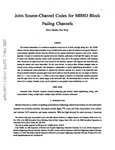
In this section, binary coded systems employing single and multiple transmit antennas are described. The general block diagram of a binary coded system over a fading channel is shown in Figure 2.1. The transmitter consists of a binary encoder (e.g., convolutional or turbo), random interleaver, a modulator and a multi-antenna transmission matrix. Time is divided into frames of 12
U
Binray Mod.
Interleaver
S
Tx Matrix Channel
Encoder
ˆ U
Decoder
DeInterleaver
Demod. Y
Figure 2.1: The structure of the binary coded system with a possible use of multi-antenna transmission. duration NT , where T is the transmission interval of a bit. Throughout the thesis, the words “sequence” and “codeword” will be used interchangeably to mean a transmission frame. In each time interval of duration kT , a rate-Rc encoder maps k information bits into n coded bits, where Rc =
k n
is the code rate.
Each coded bit is modulated to generate a signal using an equal-energy binary modulation. The modulation schemes considered in this thesis are binary phase-shift keying (BPSK) for coherent detection and binary frequency-shift keying (BFSK) for noncoherent detection. The channel we adopt is a block fading channel. Recall that in a block fading channel, each frame is subject to % signals F independent fading realizations, where a block of length m = $ N F
undergoes the same fading realization. The coded bits are interleaved prior to transmission over the channel in order to spread burst errors in the decoder, which result from low instantaneous SNR at the output of the demodulator due to fading. In the following sections, transmitters and receivers for binary coded systems employing single and multiple transmit antennas are described.
2.1.1 Single-Antenna Systems In single-antenna systems, the modulated sequence is transmitted using one antenna. Coherent or noncoherent detection can be used at the receiver to detect the received sequence. In coherent receivers, the matched filter sampled
13
output at time l in the f th fading block is given by yf,l =
! Es hf sf,l + zf,l ,
(2.1)
where Es is the average received energy, sf,l = (−1)cf,l , where cf,l is the corresponding coded bit, and zf,l is an additive white noise modeled as independent zero-mean complex Gaussian random variables with variance N0 , i.e., zf,l ∼ CN (0, N0 ). The coefficient hf is the channel gain in fading block f which
is modeled as complex Gaussian CN (0, 1) and is written as hf = af exp(jθf ), where af and θf are Rayleigh and uniform distributed, respectively.
The receiver employs maximum likelihood (ML) sequence decoding which is optimal for frame error probability. In this rule, the decoder chooses the codeword S = {sf,l , f = 1, . . . , F, l = 1, . . . , m} that maximizes the likelihood
function p(Y|S), where Y = {yf,l , f = 1, . . . , F, l = 1, . . . , m}. In coherent recep-
tion, some information about the channel phase and amplitude are available. The case where perfect SI is available at the receiver is a hypothetical scenario that predicts the best performance of the code. A practical assumption considers estimating the channel amplitude and phase resulting in imperfect SI at the receiver. This case is discussed in Chapter 3. If perfect SI is available at the receiver, the decoder chooses the codeword S that maximizes the following
metric m(Y, S) =
F " m " f =1 l=1
af sf,l Re{yf,l },
(2.2)
where Re{.} represents the real part of a complex number. In the literature, coherent detection with no amplitude SI was considered extensively as an intermediate case between coherent detection with perfect SI and noncoherent detection, where both amplitude and phase are not available at the receiver. A suboptimal decoding metric was used in [12, 34] due to its analytical tractabil-
14
ity, where the decoder chooses the codeword S that maximizes
m(Y, S) =
F " m " f =1 l=1
(2.3)
sf,l Re{yf,l }.
In noncoherent systems, BFSK signaling is used where the carrier frequency of the modulated signal is set to be one of two frequencies according to whether the coded bit c = 0, 1. The carrier frequencies are chosen such that the resultant signals are orthogonal. At the receiver, square-law combining [35] is employed for each received signal resulting in a suboptimal receiver with respect to minimizing the frame error probability. The outputs of the demodulator are represented by (I,0)
=
(Q,0)
=
(I,1)
=
(Q,1)
=
rf,l rf,l
rf,l rf,l (I,c)
where rf,l
(Q,c)
and rf,l
!
Es af δ(cf,l , 0) cos(θf ) + ηf,l
!
Es af δ(cf,l , 1) cos(θf ) + ηf,l
(I,0)
! (Q,0) Es af δ(cf,l , 0) sin(θf ) + ηf,l
(2.4)
(I,1)
! (Q,1) Es af δ(cf,l , 1) sin(θf ) + ηf,l
(2.5)
for c = 0, 1 correspond to the correlation of the received
signal with the inphase and quadrature dimensions of the signal corresponding to a coded bit c. In (2.5), θf is the unknown phase of the received signals in block (I,0)
(Q,0)
f , δ(x, y) = 1 if x = y and δ(x, y) = 0 otherwise; and ηf,l , ηf,l
(I,1)
ηf,l
(Q,1)
and ηf,l
are independent variables with N (0, N20 distribution. The decoder chooses the
codeword S that maximizes
m(R, S) =
F " m "
(I,c)
(Q,c)
(rf,l )2 + (rf,l )2 ,
(2.6)
f =1 l=1
(I,c)
(Q,c)
where R = {rf,l , rf,l , f = 1, . . . , F, l = 1, . . . , m}. Note that this decoder makes no use of channel SI in decoding.
15
2.1.2 Multi-antenna Systems In the discussion to follow we describe multi-antenna transmitters that concatenate error correcting codes with space-time block codes (STBC)s [20]. Throughout the thesis, small letters in bold are used to denote column vectors. Moreover, we consider systems employing nt transmit antennas and single receive antenna, but all derivations and results to be presented apply to multiple receive antennas. After encoding and interleaving, each nt signals are mapped into a nt × nt transmission matrix Gnt as shown below for the cases of nt = 2
and 4
s1 s2 , G2 = −s2 s1
and
s s2 s3 s4 1 −s2 s1 −s4 s3 . G4 = −s3 s4 s1 −s2 −s4 −s3 s2 s1
(2.7)
More examples of real and complex orthogonal matrices were presented in [21] for different values of nt . Note that the rows of Gnt are orthogonal to each other
to enable linear complexity detection [20]. The transmission of Gnt takes place
in a time slot of duration nt T , where the ith row of Gnt is transmitted in the ith
time interval of the time slot using the nt transmit antennas. Equivalently, the
ith column of Gnt is transmitted over the ith transmit antenna during the time
slot of duration nt T . Thus the resulting STBC has full rate, i.e., one coded bit is transmitted every T seconds. To be able to detect STBCs, the fading process from each antenna should remain constant for at least one time slot, i.e., nt time intervals. This constrains the channel memory length to be a multiple of nt , where each fading block contains
m nt
time slots each of length nt . In the rest of the thesis, the subscript
of Gnt is omitted to simplify notation. The received vector in time slot l of the
16
f th fading block is given by yf,l =
!
Es Gf,l hf + zf,l ,
(2.8)
where zf,l is a length-nt column random vector with a distribution CN (0, N0 I) and I denotes the nt × nt identity matrix. The vector hf contains the channel
gains from the transmit antennas in fading block f and is modeled as CN (0, I). This indicates that the gains from different transmit antennas are uncorre-
lated, which is reasonable if the distance separating different antennas exceeds half the wavelength of the carrier [10]. The receiver employs sequence decoding based on the detection scheme of STBC in [20]. Equivalently, the decoder chooses the codeword S that maximizes the metric
m(Y, S) =
F m/n " "t f =1 l=1
∗ Re{yf,l Gf,l hf },
(2.9)
where (.)∗ denotes the complex conjugate of a complex vector. The channel codes that are concatenated with the single and multiple antennas transmitters are described as follows.
2.1.3
Convolutional Codes
A popular channel code with an easy encoding scheme is the convolutional code. A convolutional encoder is a finite state machine consisting of v shift registers. During a time interval of length T , the encoder receives an input vector u = {ul }kl=1 of length k and produces a code vector c = {cl }nl=1 of length n.
The lth coded bit among the n coded bits at the output of the encoder is given by cl = u 1 +
v "
gl,j rj ,
mod 2,
(2.10)
j=1
where rj is the content of the j th shift register, and gl = {gl,j }vj=0 is the generator
polynomial of the lth coded bit where gl,j ∈ {0, 1}. The generator polynomials are 17
c1
u
T
T
c2 Figure 2.2: The encoder of a rate- 12 (5,7) NSC. usually expressed in octal numbers, e.g., a generator polynomial gi = 1101 is represented as gi = 15. In general, a convolutional code is represented using its generator polynomials as (g1 , g2 , . . . , gn ). The encoder for a (5,7) convolutional code is shown in Figure 2.2. This code is non-systematic code (NSC) since the coded bits are not partitioned into information (systematic) bits and parity bits. Convolutional codes which partition the information and parity bits are referred to as systematic codes. A recursive systematic code (RSC) is a systematic code with feedback in the encoder. The encoder of a RSC with k = 1 is shown in Figure 2.3. An RSC code is represented using its generator polynomials as (g1 , . . . , gn /gb ), where gb = {gb,j }vj=1 is the feedback generator polynomial. In Figure 2.3, the modified input u˜ is given by
u˜ = u +
v "
gb,j rj ,
mod 2.
(2.11)
gl,j rj ,
mod 2.
(2.12)
j=1
The coded bits are given by
cl = u˜ +
v " j=1
The frame error probability is minimized by employing a ML sequence decoder using a Viterbi algorithm [11]. The Viterbi algorithm uses the metrics described in Section 2.1.1 for different assumptions on channel SI at the receiver. 18
c1 u
T
T
u˜ c2 Figure 2.3: The encoder of a rate- 12 (5/7) RSC.
2.1.4
Turbo Codes
Originally, turbo codes referred to parallel concatenated codes [2]. The general turbo encoder is shown in Figure 2.4, which consists of two constituent codes separated by an interleaver. The constituent code can be a convolutional or a block code. If the constituent codes are block codes, the resultant code is referred to as a product code [36], where parallel concatenation of convolutional codes results in turbo codes [2]. A turbo code employing a RSC, with a respective feedforward and feedback generator polynomials of g and gb , is denoted by (1, (g/gb), (g/gb)). The information sequence is encoded by the first constituent code, and by second constituent code after being randomly interleaved. The systematic (information) sequence C as well as the parity sequences at the output of the two constituent codes, C1 and C2 are multiplexed to form a length-N codeword C. The overall code rate is Rc =
k , 2n+k
where n is the number of parity
bits at the output of each RSC and k is the number of input bits to the turbo ˜ = Rc N. encoder in each time interval. Note that the interleaver size is N The block diagram of the turbo decoder is shown in Figure 2.5. It consists of two soft-input soft-output (SISO) decoders, one for each constituent code, an interleaver similar to that used in the encoder and a deinterleaver that reverses the effect of the interleaver. The decoder works iteratively and the SISO blocks exchange soft information about information bits in each iteration. Each SISO block employs a maximum aposteriori probability (MAP) rule which 19
U C RSC
C1
Multiplexer
Interleaver
RSC
C2
Figure 2.4: The block diagram of a turbo encoder. computes the bit aposteriori probability p(ul |Y) of each bit. Using the BCJR
algorithm [2], the likelihood function of the bit ul is given by Λl = log
= log
p(ul = 1|Y) , p(ul = 0|Y) "
˜, l = 1, . . . , N !
!
!
!
(2.13)
γl (m, m )αl−1 (m )βl (m)
(m,m! ):ul =1
"
γl (m, m )αl−1 (m )βl (m)
˜ l = 1, . . . , N,
+ Λel ,
(2.14)
(m,m! ):ul =0
˜ is the length of the information sequence and γl (m, m! ) = p(ys,l , yi,l |ul ) where N
is the channel transition probability for a trellis transition from state m at time !
l to state m at time l + 1 in the ith constituent code. The first part of Λl is due to the contribution of the systematic bit and the constraint in the ith constituent code, where the second part, i.e., Λel is the extrinsic information given by Λel = log
p(ul = 1) , p(ul = 0)
˜ l = 1, . . . , N,
(2.15)
where p(ul = 0) and p(ul = 1) are the apriori probabilities for the bit ul to be 0 or 1, respectively, which are assumed to be equal in the first iteration. The !
variables αl (m ) and βl (m) are the standard forward and backward recursions in the BCJR algorithm [37]. For SISO decoder i, they are given by αl (m) = ˜
˜
N p(S l = m, {ys }l1 , {yi }l1 ) and βl (m) = p(Sl+1 = m, {ys }N l+1 , {yi }l+1 ), where p(Sl =
20
Ys
Y
DeMux Y1
SISO Dec1
{Λl }
{Λel }
SISO Dec2
Interleaver
ˆ U
Decision
{Λel }
Y2
DeInt
Figure 2.5: The turbo decoder. m, {ys }l1 , {yi }l1 ) is the joint probability density function of the encoder being at state m at time l and the sequences {ys }l1 and {yi }l1 . A similar definition holds ˜
˜
N for the function p(Sl+1 = m, {ys }N l+1 , {yi }l+1 ). The variables αl (m) and βl (m) are
computed in each SISO decoder, respectively as αl (m) =
"
!
!
γl (m, m )αl−1 (m ),
˜ l = 1, . . . , N,
(2.16)
!
m
βl (m) =
"
!
!
γl+1(m, m )βl+1 (m ),
˜ l = 1, . . . , N.
(2.17)
!
m
In the final iteration, a decision is made on information bits according to
uˆl =
2.2
0, if Λl ≤ 0, 1, if Λl > 0.
(2.18)
Space-Time Coded Systems
In this section we describe the ST coded systems. The section starts with a general system description. Then, trellis and turbo ST codes are discussed. The block diagram of the general ST coded system is shown in Figure 2.6. The transmitter consists of a ST encoder, an interleaver, a modulator and nt transmit antennas. During a frame transmission period of length NT , the input to the transmitter is a length-N sequence U = {ul }N l=1 of input vectors each of
length k. Each component of the input vector ul is assumed to be from a binary
21
S
ST Encoder
Interleaver
Modulator
Decoder
DeInterleaver
Demod.
Channel
U
ˆ U Y
Figure 2.6: A general ST coded system. alphabet. The ST encoder produces a length-N sequence S = {sl }N l=1 of signal
vectors each of length nt . The ith element of each signal vector sil is an element of an M-ary signal constellation, such as MPSK or M-QAM, which is modulated and transmitted using the ith transmit antenna in the time interval l. Therefore, the overall system throughput is k/T bits/s. Before being modulated, the signal vectors are interleaved to avoid burst errors in the decoder. Note that we used s instead of c to denote the output of the encoder because each element of s is a signal from a constellation as opposed to being a coded bit in the case of binary codes. This notation is used for ST coded systems throughout the thesis. The received signal at time interval l in fading block f is yf,l =
!
Es
nt "
hif sif,l + zf,l ,
(2.19)
i=1
where Es is the average transmitted energy at each transmit antenna and zf,l is an additive white noise modeled as CN (0, N0 ). The coefficient hif is the chan-
nel gain from the ith transmit antenna in fading block f , which is modeled as CN (0, 1). As in the case of STBCs, it is assumed that the channel gains from
different transmit antennas are uncorrelated, i.e. E[hpf hq∗ f ] = 0 for p *= q, where
(.)∗ denotes the complex conjugate. The decoder employs a ML decoding rule to minimize the frame error probability. Assuming perfect channel SI at the
22
u1
T
T a12
a11
a10
s1
Add mod M s2 a21
a20
u2
a22
T
T
Figure 2.7: The encoder of a trellis ST code with k = 2 and v = 4. receiver, the ML decoding rule chooses a codeword S that maximizes nt F " m -2 " ! " hif sif,l - . m(Y, S) = − -yf,l − Es
(2.20)
i=1
f =1 l=1
2.2.1 Trellis ST Codes
The trellis an ST encoder considered in this thesis consists of k parallel trellis subcodes, each encodes one of the k input bits. The resulting code has a throughput of k/T bits/s. This is a generalization of the encoder described in [38]. In general, each subcode has v˜ shift registers. The contents of the shift ˜ , for q = 1, . . . , k. Note that registers of the q th subcode are denoted by {rlq }vl=1
the total code memory is v = k˜ v . Figure 2.7 shows a trellis encoder with k = 2 and v = 4. The signal vector at the output of the encoder at time l is given by
sl =
k " v˜ "
ul−j aql−j
mod M,
(2.21)
q=1 j=1
t is a length-nt vector with elements drawn from a set with where aq = {aq,i}ni=1
cardinality M, i.e., aq,i ∈ {0, 1, . . . , M − 1}.
For the purpose of iterative joint decoding and channel estimation to be
discussed in Chapter 5, a SISO decoder is necessary. Using the BCJR algorithm 23
[37], soft information about signal vectors in the frame is computed using / . p sl -Y, H = C
"
!
!
γl (m, m )αl−1 (m )βl (m),
l = 1, . . . , N,
(2.22)
(m,m! ):sl !
where C is a normalization constant, γl (m, m ) = p(yl |sl , hl ) is the branch metric !
for a trellis transition from state m at time l to state m at time l + 1, where
hl contains the channel gains of the fading block in which time interval l lies. The variables αl and βl are the standard forward and backward recursions in the BCJR algorithm computed as in Section 2.1.4.
2.2.2 Turbo ST Codes In [39], Yuan et al. presented ST turbo scheme consisting of two constituent codes and an interleaver as shown in Figure 2.8. During a transmission interval of length NT , the input to the encoder is a length-N/2 sequence of inforN/2
mation vectors U = {ul }l=1 , each of length k bits. The information sequence N/2
is encoded using the first constituent code into S1 = {sl }l=1 . The information
sequence is randomly interleaved and encoded by the second constituent code into S2 . The two signal sequences out of the constituent codes are multiplexed to form the signal frame S = {sl }N l=1 . Hence, the throughput of the resultant
turbo code is
k 2
bits/s.
The constituent codes are recursive trellis ST codes that output signal vectors of length nt , with elements from an M-ary signal constellation [39]. Figure 2.9 shows a recursive ST trellis with k = 2 and v = 4. In the lth time interval, the q th recursive subcode in the ST encoder generates a modified input bit as r0q
= ul +
v˜ "
q rl−j
j=1
24
mod 2.
(2.23)
S1
Recursive ST Encoder over M set
U
Multiplexer
S
Vector Interleaver
S2
Recursive ST Encoder over M set
Figure 2.8: The structure of a turbo ST encoder. The output signal vector is given by
sl =
k " v˜ "
mod M,
q rl−j aql−j
(2.24)
q=1 j=1
where ah is the same as that for non-recursive trellis ST codes. The decoder of ST turbo codes is based on the turbo decoding principle [2], in which two SISO modules are used, one for each constituent code. Aposteriori probabilities of input vectors in the frame are computed as / . p ul -Y, H = K
"
!
!
γl (m, m )αl−1 (m )βl (m),
l = 1, . . . , N,
(2.25)
!
(m,m ):ul
!
where γl (m, m ) = p(yl |ul , hl )p(ul ) and p(ul ) is the apriori probability of the input vector ul computed in the other SISO block, which is set equal for all input
vectors in the first iteration. Information passed between the SISO modules is extrinsic information which is the probability in (2.25) after removing the contribution of p(ul ). The algorithm runs for a number of iterations, and in the last iteration the decoder chooses the information vector with the largest aposteriori probability. For the purpose of iterative decoding and channel estimation,
25
u1
T a10
a11
T a12
Add mod M a20
u2
a21
T
s
a22
T
Figure 2.9: The encoder of a recursive trellis ST code with k = 2 and v = 4. SISO modules compute soft information about signal vectors using (2.22).
26
CHAPTER 3 Performance of Binary Coded Systems over Rayleigh Block Fading Channels
In this chapter, a union bound for binary coded systems over block fading channel is derived. Systems employing single and multiple transmit antennas are considered. Conventionally, the performance of coded systems over ideally interleaved channels is analyzed using the union bound, which was computed by Viterbi [11] for specific convolutional codes using the weight enumerator of the code. In [12], Divsalar et al. derived similar bounds for trellis codes with perfect and no amplitude SI assumptions, where union bound for turbo codes were presented by Hall et al. [5]. Multi-frequency trellis codes [40] are special codes for block fading channels. At each state transition in multi-frequency trellis codes, the encoder produces signals, each is transmitted over one fading block. Hence, the number of output signals at each transition equals the number of fading blocks in the frame. This makes these codes too complicated for arbitrary number of fading blocks. In [41], the union bound for multi-frequency convolutional codes was evaluated. Several block and trellis codes designed for the block fading channels were presented in [42]. Also, in [42], Knopp et al. derived the outage probability of binary coded systems over block fading channels. Malkamaki et al. [43] derived random coding upper bounds on the average error probability of coded diversity over block fading channels. Also, an
27
expression for the maximum achievable diversity as a function of the number of fading blocks and the code rate was presented. Despite the efforts to analyze the performance of coded systems over block fading channels, a method for evaluating the error probability of binary codes is needed. In this chapter, we derive a union bound on the error probability of binary coded systems over block fading channels. Using the union bound the channel memory can be optimized for a coded system employing iterative decoding and channel estimation. This chapter is organized as follows. In Section 3.1 the union bound for communication systems employing arbitrary convolutional and turbo codes over block fading channels is derived. Communication systems employing single and multiple transmit antennas are considered in Sections 3.2 and 3.3, respectively. Expressions for pairwise error probability of the coded systems are derived for noncoherent and coherent receivers with different assumptions about the channel SI at the receiver. Results are presented and discussed for each case following the derivation of the corresponding result.
3.1
Union Bound
In this section, a union bound on the bit and frame error probability of convolutional and turbo codes over block fading channels is derived. Throughout the thesis, the subscripts c, u and b are used to denote conditional, unconditional and bit error probabilities, respectively. For linear convolutional codes with k input bits, the bit error probability is upper bounded [11] as N 1 " wd Pu (d), Pb ≤ k
(3.1)
d=dmin
where dmin is the minimum distance of the code, Pu (d) is the unconditional pairwise error probability defined as the probability of decoding a received sequence as a weight-d codeword given that the all-zero codeword is transmitted. 28
In (3.1), wd =
0N
i=1
iAi,d is the number of codewords with output weight d, where
Ai,d is the number of codewords with output weight d and input weight i. The weight distribution {wd }N d=dmin is obtained directly from the weight enumerator ˜ = Rc N, the union of the code [11]. For turbo codes with code interleaver size N
bound for a particular interleaver is difficult to evaluate. However, if we consider the ensemble of codes generated by all possible interleavers, then we can obtain a bound on the bit error probability of such a code by averaging over all possible interleavers [44] ˜ 1 ˜2 " N N " i N p(i, d)Pu (d), Pb ≤ ˜ i N i=1 d=d
(3.2)
min
where p(i, d) is the probability of having an input sequence with weight i and an output codeword with weight d. For a turbo code with two component codes, p(i, d) is given by "
p(i, d) =
p0 (i, d0 )p1 (i, d1 )p2 (i, d2 ),
(3.3)
{d0 ,d1 ,d2 }:d0 +d1 +d2 =d
where p0 (i, d0 ) = δ(i, d0 ) represents the systematic bit; and pj (i, dj ) = Ai,dj /
.N˜ / i
for j = 1, 2, accounts for the code interleaver. The frame error probability of turbo codes is given by
Pf ≤
˜ 1 2 N N " ˜ " N i=1
i
p(i, d)Pu (d).
(3.4)
d=dmin
3.1.1 Union Bound for Block Fading Channels Recall that in the block fading channel model, a frame of size N is affected by F fading realizations. Thus the fading realization stays constant for a dura% signals. In this case, the pairwise tion of a fading block composed of m = $ N F
error probability Pu (d) is a function of the distribution of the d nonzero bits
over the F fading blocks. In the following, this distribution is quantified as29
suming uniform channel interleaving of the coded bits over the fading blocks. Figure 3.1 shows the distribution of the d nonzero bits in a weight-d erroneous codeword over the F fading blocks. Denote the number of fading blocks with weight v by fv and define w = min(m, d), then the fading blocks are distributed according to the pattern f = {fv }w v=0 if the following conditions are satisfied F =
w "
fv ,
w "
d=
v=0
(3.5)
vfv .
v=1
Denote by L = F − f0 the number of fading blocks with nonzero weights. Then Pu (d) averaged over all possible fading block patterns is given by d "
Pu (d) =
L2 L1 " "
...
L=#d/m$ f1 =1 f2 =1
where
3
Lv = min L −
v−1 "
fr ,
d−
r=1
Lw "
Pu (d|f)p(f),
(3.6)
fw =1
0v−1
r=1 rfr v
4
,
1 ≤ v ≤ w.
(3.7)
The probability of a fading block pattern p(f) is computed using combinatorics as p(f) =
.m/f1 .m/f2 1
... 2 .mF / d
.m/fw w
.
F! . f0 !f1 ! . . . fw !
(3.8)
The left factor of p(f) in (3.8) is the probability of distributing d nonzero bits over F blocks with fv blocks having v bits, for possible values of v. The right term of p(f) is the probability of having such combinations f = {fv }w v=0 among
the F fading blocks. Using (3.6)-(3.8), the union bounds on the bit error probabilities of convolutional and turbo codes over a block fading channels are found by substituting (3.6) in (3.1) and (3.2), respectively. Also, substituting (3.6) in (3.4) results in the union bound on the frame error probability of turbo codes over block fading channels. The number of summations involved in computing Pu (d) in (3.6) increases as the channel memory length increases. Computing the bound by summing all values of d ≤ N for a large channel memory length becomes a time consum30
d nonzero bits
…………… d1 bits
d2 bits
Block 1
0 bits … …
Block 2
0 bits 1 bits … …
f0 Blocks
……………
dF-1 bits
……………
Block(F-1)
1 bits
……………
f1 Blocks
dF bits Block F
w bits … … w bits
……………
fw Blocks
Figure 3.1: The distribution of the d nonzero bits in a d-weight error codeword over the F fading blocks. ing task. However, a good approximation to the union bound is obtained by truncating it for a small value of d < N. This results in an approximation to the error probability rather than an upper bound.
3.1.2 Pairwise Error Probability The conditional pairwise error probability Pc (d|f) is defined as the probaˆ given that bility of decoding a received sequence Y as a weight-d codeword S the all-zero codeword S was transmitted and conditioned on the channel fading gains. It is given by 5 6 ˆ Pc (d|f) = Pr m(Y, S) − m(Y, S) < 0 H, S ,
(3.9)
where H = {hf }Ff=1 . Note that the d nonzero errors are distributed over the F
fading blocks according to a pattern f. For a specific receiver, the unconditional pairwise error probability Pu (d|f) is found by substituting the corresponding
decoding metric (3.9) and then averaging over the fading gains. The rest of this chapter is devoted to deriving expressions of the unconditional pairwise error 31
probability for coded single and multiple transmit antennas systems employing different receivers with different SI assumptions at the receiver.
3.2
Single-Antenna Systems
In this section, the pairwise error probability Pu (d|f) is derived for coded single-antenna systems employing coherent and noncoherent receivers. For coherent detection, we consider the cases of perfect and imperfect SI at the receiver as well as the case of no amplitude SI. For noncoherent detection, receivers employing a square-law combining are considered.
3.2.1 Coherent Detection - Perfect SI Recall that the received signal over a block fading channel is given by (2.1) and the corresponding ML decoding rule is given by (2.2). Substituting the metric (2.2) in (3.9), the conditional pairwise error probability for coherent detection with perfect SI is given by
Pc (d|f) = Pr
7
L " f =1
af
m " l=1
8 Re{yf,l } < 0-H, S .
The distribution of Re{yf,l } conditioned on af is Gaussian with mean
(3.10) √
Es af sf,l
and variance N0 . The conditional pairwise error probability simplifies to 9 : fv w : " " v a2i , Pc (d|f) = Q ;2Rc γb v=1
where γb =
Eb N0
(3.11)
i=1
is the SNR per information bit. Note that the average energy
per bit is given by Eb = Rc Es , where Rc is the encoder rate. To find Pu (d|f),
32
(3.11) is averaged over the fading amplitudes as 9 : fv w : " " Pu (d|f) = EA Q ;2Rc γb v a2i , v=1
(3.12)
i=1
where A = {af }Ff=1 . Using the Chernoff bound, Q(x) ≤ 12 e−x
2 /2
, the uncondi-
tional pairwise error probability is upper bounded as w
1@ Pu (d|f) ≤ 2 v=1
1
1 1 + vRc γb
2fv
(3.13)
,
where the product results from the independence of fading in different fading blocks. An exact expression of the pairwise error probability can be found by Aπ 2 2 using the integral expression of the Q-function, Q(x) = π1 02 e(−x /2 sin θ) dθ [45] 1 Pu (d|f) = EA π 1 = π
C
0
BC
π 2
π 2
exp
0
w 1 @ v=1
7
w
fv
Rc γb " " 2 v a sin2 θ v=1 i=1 i
1 1 + vRc γb / sin2 θ
2 fv
8
dθ.
dθ
D
(3.14)
The union bound was evaluated for a rate- 12 (23,35) convolutional code with a frame size of N = 2 × 512 coded bits, and a rate- 13 (1,5/7,5/7) turbo code with
a frame size N = 3 × 1024 coded bits. Note that the convolutional code has
4 memory elements, whereas the component codes of the turbo have 2 mem-
ory elements. As discussed in Section 3.1.1, the union bound is truncated to reduce computation complexity. For convolutional codes, the union bound was truncated after codewords with distances d > 12. However, the union bound for turbo codes was truncated after d > 52. The bound is compared to simulation results. In the simulations, the channel interleaver is chosen randomly and is changed every 10 frames to account for the uniform interleaving argument. In turbo codes, the code interleaver is an s-random interleaver. In the literature, s-random interleavers are used due to their good performance. An s-random in-
33
terleaver permutes the data sequence in such a way that bits within distance of s from each other are separated by more than s positions in the interleaved sequence. In coherent systems, BPSK signaling is employed and (3.14) is used to compute the union bound. Figure 3.2 shows the results for the convolutional code with perfect SI for channel memory ranging from m = 1 to m = 64. In the figure we plot the curves corresponding to simulation and union bound results. Since simulating very low error rates is too difficult, we plot simulation curves up to error rates of around Pb = 10−6 . However, the union bound curves are plotted for all SNR values. From the figure, the bound is very close to the simulation curves for a wide range of channel memory lengths. Also, the union bound starts to be loose as the SNR decreases, where the union bound is known to diverge at SNR values lower than the cutoff rate of the channel [46]. However, since simulation is easy for low error rates, the importance of the performance analysis is emphasized at high SNR values. In the following results, the union bound is plotted for high SNR values to make the presentation more clear. The frame error probability of the turbo code is shown in Figure 3.3. We observe that the bound is able to predict the performance loss due to channel memory in the error floor region, i.e., at the high SNR. Also, the bound is not as close to simulation results as in the case of convolutional codes. This is mainly because the turbo code interleaver is an s-random interleaver, where the union bound for turbo codes in (3.4) assumes uniform code interleaver which averages the performance of bad and good code interleavers. However, using the bound provide some insight about the performance of turbo codes with channel memory. Note that the performance of turbo codes in the water-fall region is not predictable using the distance spectrum of the code. In this region iterative decoding is the major influence on the performance and results for ML decoding does not hold. Generally, the performance with perfect SI degrades as the channel memory increases.
34
!1
10
m=1 m=8 m=16 m=32 m=64
!2
10
!3
10
!4
10
!5
10
Pb !6
10
!7
10
!8
10
!9
10
!10
10
4
6
8
10
12
14
16
γb (dB)
Figure 3.2: Bit error probability of a rate- 12 (23,35) convolutional code with perfect SI and a frame size N = 1024 for channel memory lengths m = 1, 8, 16, 32, 64 (solid: approximation using the union bound, dash: simulation). 0
10
m=1 m=8 m=16 m=32 m=64
!1
10
Simulation
!2
10
!3
10
!4
10
Pf
!5
10
!6
10
!7
10
Approximation
!8
10
!9
10
!10
10
2
4
6
8
10
12
14
γb (dB)
Figure 3.3: Frame error probability of a rate- 13 (1,5/7,5/7) turbo code with per˜ = 1024 for channel memory lengths fect SI and an code interleaver size N m = 1, 8, 16, 32, 64. 35
3.2.2 Coherent Detection - Imperfect SI For coherent detection with imperfect SI it is necessary to estimate the channel SI. This is achieved by transmitting a pilot signal with energy Ep in each fading block. The corresponding received signal is given by ! Ep hf + zf,p .
yf,p =
(3.15)
yf,p z ˆf = √ = hf + ef , where ef = √f,p The ML estimator for hf is given by h Ep
is the estimation error. The distribution of ef is
Ep
CN (0, σe2 )
where
σe2
=
N0 . Ep
The
correlation coefficient between the actual channel gain and its estimate is given by ˆ∗ ] E[hf h 1 f . =! µ= E 2 1 + σ ˆ e Var(hf )Var(hf )
(3.16)
In order implement a ML decoding rule, the likelihood function of the channel observations (received and pilot signals) conditioned on the transmitted codeword should be maximized. Define yp = {yf,p}Ff=1 to be the vector containing
pilot signals in a frame, then the likelihood function is written as
p(Y, yp |S) = EH [p(Y, yp|H, S)] = C1
F C @
f =1
∞
0
1
! 1 exp − |yf,p − Ep hf |2 N0
8 m ! 1 " 2 |yf,l − Es hf sf,l |2 e−|hf | dhf , × exp − N0 l=1 7
2
(3.17)
(3.18)
where C1 is a constant. Simplifying
6 " 1 2 2 p(Y, yp |S) = C2 exp − (|yf,p | + |yf,l | ) N0 f =1 l=1 F @
C
5
m
F 6G 1 5 α|hf |2 − 2Re{h∗f βf } dhf , exp − (3.19) N0 0 ! √ 0 ∗ where α = Ep + mEs + N0 , βf = Ep yf,p + Es m l=1 yf,l sf,l and C2 is another ×
∞
constant. Simplifying and completing the squares by adding and subtracting 36
|βf |2 αN0
results in
p(Y, yp |S) = C3
F @
exp
f =1
5
−
6 5 1 6 " 1 (|yf,p|2 + |yf,l |2 ) exp |βf |2 N0 αN0 l=1
×
C
m
∞ 0
5 α -βf --2 6 h exp − − - dhf , - f N0 α
(3.20)
where C3 is a constant. Now, the integral becomes a constant since it is an integral of a Gaussian density function. Note that the only part that depends on the transmitted codeword is the second exponential term. Thus based on observing the received and the pilot signals, the ML decoder chooses the codeword S that maximizes the metric m(Y, S) =
F " f =1
2
|βf | =
F " f =1
Es |
m " l=1
yf,l s∗f,l |2
ˆ f have been substituted for where h
m ! " ∗ ˆ f } + C4 , + 2 Es Re{yf,l sf,l h
(3.21)
l=1
! Ep yf,p and C4 is another constant term
that is independent of the transmitted codeword. This receiver is difficult to implement in a Viterbi decoder of a convolutional code. Also, it is difficult to analyze. Therefore, a suboptimal decoding metric that maximizes the likeliˆ S) is used. It is given by hood function p(Y|H,
m(Y, S) =
F " m " f =1 l=1
∗ ˆ Re{yf,l hf sf,l }.
(3.22)
In order to find the pairwise error probability, the distribution of the reˆ f is required. Apceived signal yf,l conditioned on the estimated channel gain h plying basic probability results, this distribution is found to be a complex Gaus√ ˆf ) = ˆ f sf,l and variance N0 + (1 − µ2 )Es , where σ 2 = Var(h sian with mean µσ Es h
37
Table 3.1: Rates, minimum distances and puncturing patterns of the punctured rate- 12 codes. m 4 8 16 32 64
˜c Code Rate R 0.667 0.571 0.533 0.516 0.508
Puncturing Location 3 7 15 31 63
dmin 4 5 6 6 6
1 + σe2 . Thus the conditional pairwise error probability becomes 9 : fv w " " : : 2µ2 R γ v |ζi|2 c b : ; v=1 i=1 , Pc (d|f) = Q 2) 1 + R γ (1 − µ c b where ζ =
ˆ h . σ
Define γˆb =
µ2 γb 1+Rc γb (1−µ2 )
(3.23)
to be the effective SNR after taking
into account the additional noise in the channel estimation, the unconditional pairwise error probability simplifies to (3.14) with γb replaced by γˆb . Two scenarios can be considered for channel estimation using pilots with Ep = Es . The first one results from only pilot estimation (OPE) with an estimation error variance of σe2 =
N0 . Es
The second case considers a lower bound on the
performance of receivers employing iterative joint decoding and channel estimation. In such receivers the decoding results are used to improve the channel estimates, which are used to improve the decoding results. This process is repeated iteratively. In general, the more reliable the decoding results, the more accurate is channel estimation. A lower bound on the performance of iterative receivers is obtained if the signals in each fading block are known with probability one. In this case they can be considered as pilots resulting in an estimation error variance of σe2 =
N0 . mEs
This case is referred to as correct data
estimation (CDE). Similar channel estimation scenarios were used in [47–49] for channel estimation for LDPC codes. 38
In simulating systems with channel estimation via pilot insertion, one coded bit is punctured every m coded bits to account for the rate reduction resulting from inserting a pilot signal every m−1 signals. This affects the whole distance distribution of the resulting code and may reduce the minimum distance of the code. In general, the resultant code rate after puncturing is given by ˜ c = mRc , R m − np
(3.24)
where np is the number of pilot signals inserted in each fading block which is set to be np = 1 in single-antenna systems. In Table 3.1 we show the code rates and the minimum distances of the punctured codes for different channel memory lengths. Also, the location of the punctured coded bit in a m-length fading block. According to the table, the code rate increases with reducing the channel memory length, which decreases the error correcting capabilities of the code. Thus systems with short channel memory are expected to have more channel diversity at the cost of lower minimum distance and worse channel estimation quality. On the other hand, longer channel memory results in more a powerful code as well as better channel estimation at the cost of less channel diversity. Figures 3.4 and 3.5 show the results for convolutional code with imperfect SI under the OPE and CDE assumptions, respectively. Note that the energy of the pilot is taken into account in the SNR axis. We observe that the SNR degradation due to channel memory is less compared to the case of perfect SI. This is expected since the number of transmitted pilot signals is reduced as the channel memory gets longer, and hence the system becomes more energy efficient. Also, the estimation quality under the CDE assumption improves with increasing channel memory length as appears in the expression of σe2 . From the figures, the cases of m = 16 and m = 32 are the best systems, where the former becomes better than the later for an SNR values exceeding 14 dB. This suggests that the optimal channel memory length is between m = 16 and
39
!1
10
m=4 m=8 m=16 m=32 m=64
!2
10
!3
10
Simulation
!4
10
Pb
!5
10
!6
10
Approximation
!7
10
!8
10
!9
10
4
6
8
10
12
14
16
18
20
γb (dB)
Figure 3.4: Bit error probability of a (23,35) convolutional code with imperfect SI (OPE receiver with Ep = Es ) and a frame size N = 1024 for channel memory lengths m = 4, 8, 16, 32, 64. !1
10
m=4 m=8 m=16 m=32 m=64
!2
10
!3
10
!4
10
Pb
Simulation
!5
10
!6
10
Approximation
!7
10
!8
10
!9
10
4
6
8
10
12
14
16
18
20
γb (dB)
Figure 3.5: Bit error probability of a (23,35) convolutional code with imperfect SI (CDE assumption with Ep = Es ) and a frame size N = 1024 for channel memory lengths m = 4, 8, 16, 32, 64. 40
0
10
m=4 m=8 m=16 m=32 m=64
!1
10
Simulation
!2
10
!3
10
Pf
!4
10
!5
10
Approximation
!6
10
!7
10
!8
10
2
4
6
8
10
12
13
γb (dB)
Figure 3.6: Frame error probability of a (1,5/7,5/7) turbo code with imperfect SI ˜ = 1024 for channel (OPE receiver with Ep = Es ) and an code interleaver size N memory lengths m = 4, 8, 32, 64. m = 32. Also, the cases of m = 8 is the worse than the case of m = 64 at low SNR and starts to improve as the SNR increases. This is because the resulting code for m = 8 is less powerful than the code for m = 64 but has larger amount of channel diversity. Although the case of m = 64 has the best code, it lacks enough channel diversity to perform better than the other cases. Under the CDE assumption, the case of m = 64 performs the best at low SNR because longer memory permits better estimation. In general, the optimal memory tends to increase under the CDE assumption compared to the OPE receiver due to the improved channel estimation. In all cases the channel memory m = 4 performs the worst because the resulting code is weak due to puncturing one coded bit every 4 coded bits. Results for turbo code with imperfect SI using an OPE receiver and the CDE assumption are shown in Figures 3.6 and 3.7, respectively. In OPE receivers, we observe that the curves of the cases of m = 8, 16, 32 cross at different SNR points. As the SNR increases, short channel memory provides better perfor41
0
10
m=4 m=8 m=16 m=32 m=64
!1
10
Simulation
!2
10
!3
10
Pf
!4
10
!5
10
!6
10
Approximation
!7
10
!8
10
1
2
4
6
8
10
12
γb (dB)
Figure 3.7: Frame error probability of for a (1,5/7,5/7) turbo code with imperfect ˜ = 1024 for SI (CDE assumption with Ep = Es ) and an code interleaver size N channel memory lengths m = 4, 8, 32, 64. mance than long channel memory, which is apparent in the analytical curves. From this we conclude that the optimal memory length changes with the operating SNR value. In the CDE assumption, the channel memory lengths m = 32 and m = 64 are very close where the former becomes the best at high SNR. Figure 3.8 shows a comparison between the performance of the convolutional code with channel memory lengths m = 8 and m = 32 for the cases of perfect SI, OPE receiver and the CDE assumption. It is clear that as the channel memory gets longer, the SNR degradation due to imperfection in the channel SI reduces. This is because long channel memory causes less penalty in the rate and energy than short channel memory does, as well as an improved channel SI under the CDE assumption. When the energy allocated for the pilot signal is varied, the performance of an OPE receiver is expected to change as a function of the channel memory. The energy per information bit is written as a function of the energy allocated
42
!2
10
perf CDE OPE !3
10
!4
10
!5
10
Pb !6
10
!7
10
!8
10
!9
10
6
8
10
12
14
16
18
γb (dB)
Figure 3.8: The performance of convolutional coded systems with a frame size N = 1024 and channel memory lengths m = 8, 32 using perfect and imperfect SI with Ep = Es (solid: m = 8, dash: m = 32). 16
15
m=8 m=16 m=32 m=64
γb (dB)
14
13
12
11
10
9 !4
!2
0
2
4
6
8
10
12
14
16
Ep /Es (dB)
Figure 3.9: SNR required for the (23,35) convolutional code to achieve Pb = 10−4 versus Ep /Es for the OPE receiver and channel memory lengths m = 8, 16, 32, 64. 43
for transmitting signals and pilots as Eb =
(m − np )Es + np Ep . mRc
(3.25)
Thus for a fixed channel memory, there exists an optimal value for pilot energy. This is illustrated in Figure 3.9, where the SNR required for the system to achieve bit error probability of Pb = 10−4 is plotted versus the pilot-to-signal energy ratio Ep /Es in dB. We observe that as the channel memory length increases the optimum value for Ep /Es increases. This is expected since longer channel memory permits more possible energy to be allocated for the pilot signal. On the other hand, when the channel memory is short, a more wise usage of the offered energy is to transmit the information signals rather than to estimate the channel. Note that optimizing the pilot energy results in an SNR gain as large as 1 dB over the case where Ep = Es . This SNR gain increases as the channel memory increases since longer memory increases the amount of energy that can be devoted for channel estimation, which improves the overall performance.
3.2.3
Coherent Detection - No Amplitude SI
For completeness we consider the case where the channel phase is known but the amplitude is unknown. A suboptimal decoding metric (2.3) is used due to its mathematical tractability. Substituting this metric (3.9) and using the Chernoff bound to upper bound the pairwise error probability [12] as
Pc (d|f) ≤
L @
f =1
F
5
Ey exp − 2λ
m " l=1
Re{yf,l }|sf,l − sˆf,l |
6G ,
(3.26)
where λ > 0 is the Chernoff parameter. Following the derivation in Appendix A.1, the pairwise error probability with coherent detection and no amplitude
44
!1
10
m=1 m=8 m=16 m=32 m=64
Simulation
!2
10
!3
10
!4
10
Pb
!5
10
!6
10
!7
10
Approximation
!8
10
!9
10
4
6
8
10
12
14
16
18
γb (dB)
Figure 3.10: Bit error probability of a rate- 12 (23,35) convolutional code with no amplitude SI and a frame size N = 1024 for channel memory lengths m = 1, 8, 16, 32, 64. SI is given by Pu (d|f) !
1
ed 2Rc γb L
2 L 7@ w v=1
v
2fv
8−1
,
(3.27)
where e = exp(1). The union bound is evaluated for the case of coherent detection with no amplitude SI using (3.27) and results are shown in Figure 3.10. From the figure, we observe that the bound is less tight than in the perfect SI case. This is due to the use of the Chernoff bound which is known to be a little loose in low SNR region. However, it dictates the trend in the performance over block fading channels, where the SNR degradation due to memory is clear and close to that shown in simulations.
3.2.4
Noncoherent Detection
In noncoherent systems the channel phase is unknown at the receiver. A receiver that does not need any channel estimation (phase and amplitude) is
45
the square-law combining receiver. Recall that the outputs of the square-law combiner are given by (2.5) and the corresponding decoding metric appears in (2.6). The conditional pairwise error probability is found by substituting the metric (2.6) in (3.9)
Pc (d|f) = Pr
1" F f =1
2 5 6 (I,1) 2 (Q,1) 2 (I,0) 2 (Q,0) 2 df |rf | + |rf | − |rf | − |rf | > 0-H, S ,
(3.28)
where df is the number of error bits in the fading block f . The variables (I,0)
{rf
(Q,0)
, rf
(I,1)
} and {rf
(Q,1)
, rf
} are zero mean Gaussian random variables with (s)
(I,s)
(Q,s)
variances equal to 12 (Es + N0 ) and 12 N0 , respectively. Let |rf |2 = |rf |2 + |rf |2 F " (1) (0) for s = 0, 1 and define κ = df (|rf |2 − |rf |2 ). Then, the unconditional pairf =1
wise error probability is upper bounded using the Chernoff bound and the density function p(κ) as Pu (d|f) =
C
∞ 0
H I p(κ)dκ ≤ Eκ eλκ ,
(3.29)
where λ > 0 is the Chernoff parameter that should be optimized to result in the tightest bound. Substituting for κ and collecting terms having the same distance Pu (d|f) ≤
w G G F F @ (1) 2 fv (0) 2 fv E eλv|rv | E e−λv|rv | .
(3.30)
v=1
The Chernoff parameter λ is optimized as in [35] and the resulting Chernoff bound for the pairwise error probability simplifies to Pu (d|f) ≤ where Dv =
1 . 2+vRc γb
w @ v=1
[4Dv (1 − Dv )]fv ,
(3.31)
The union bound for convolutionally encoded BFSK sig-
nals with square-law combining is evaluated using (3.31) and shown in Figure 3.11. The bound is less tight than the perfect SI case due to the use of the Chernoff bounding technique. However, the performance trend and the SNR
46
!1
10
m=1 m=8 m=16 m=32 m=64
!2
10
Simulation
!3
10
!4
10
!5
10
Pb !6
10
!7
10
Approximation
!8
10
!9
10
!10
10
8
10
12
14
16
18
20
γb (dB)
Figure 3.11: Bit error probability of a rate- 12 (23,35) convolutional code with noncoherent detection and a frame size N = 1024 for channel memory lengths m = 1, 8, 16, 32, 64. degradation due to memory are predicted well from the bound.
3.3
Multi-Antenna Systems
In this section, the pairwise error probabilities for coded STBC systems are derived. Coherent detection with perfect and imperfect SI is considered. Note that the results for the case of perfect SI apply directly to coded differential STBCs taking into account a penalty of 3 dB in the SNR [22].
3.3.1 Perfect SI Recall that the received vector due to transmitting a STBC transmission matrix Gf,l is given by (2.8). Also, the simple decoding metric that is equivalent
to ML metric is given by (2.9). The conditional pairwise error probability for coded STBCs with perfect SI is found by substituting the metric (2.9) in the
47
expression of the pairwise error probability in (3.9) resulting in
Pc (d|f) = Pr
7
L " w "
κf,l
f =1 l=1
8 < 0-H, S ,
(3.32)
∗ where κf,l = Re{yf,l Ef,l hf } and Ef,l = Gf,l − Gˆf,l . Here, Gf,l and Gˆf,l are the
transmission matrices in time slot l of the f th fading block corresponding to the all-zero codeword and a weight-d error codeword, respectively. We use (.)∗ and (.)T to denote the complex conjugate of a complex vector and the transpose of a real matrix, respectively. In (3.32), κf,l is a Gaussian random variable with conditional mean and variance given respectively by nt " I ! K ! J H T Ef,l hf = Es df,l |hif |2 , E κf,l -Gf,l , hf = Es Re h∗f Ef,l
(3.33)
i=1
nt " I H J ∗ KI ∗ T Var κf,l Gf,l , hf = E Re zf,l Ef,l hf hf Ef,l zf,l Gf,l , hf = df,l N0 |hif |2 ,
H
(3.34)
i=1
where df,l is the number of error bits in the time slot l in the f th fading block. In (3.33) and (3.34), the cross terms are zero due to the orthogonality of the rows in Ef,l . The error probability in (3.32) simplifies to 9 : fv nt w : " " " v |hil |2 . Pc (d|f) = Q ;2Rc γb v=1
(3.35)
l=1 i=1
As in Section 3.2.1, the unconditional pairwise error probability Pu (d|f) is found by averaging over the fading gains and using the exact expression of the Q function. The resulting expression of Pu (d|f) is given by 1 Pu (d|f) = π
C
0
π 2
w 1 @ v=1
1 1 + vRc γb / sin2 θ
2nt fv
dθ.
(3.36)
As study cases, a rate- 12 (23,35) convolutional code with 4 memory elements is concatenated with a STBC employing two and four transmit antennas with the
48
!1
10
m=2 m=16 m=32 m=64 m=128
Simulation
!2
10
!3
10
!4
10
!5
10
Pb !6
10
!7
10
Approximation
!8
10
!9
10
!10
10
2
3
4
5
6
7
8
9
10
11
12
γb (dB)
Figure 3.12: Bit error probability of a convolutionally coded STBC with perfect SI, nt = 2 and a frame size N = 1024 for channel memory lengths m = 2, 16, 32, 64, 128. same simulation settings as in the single-antenna case. The union bound was evaluated by substituting (3.36) in (3.1) and summing over codewords with distances d ≤ 12 for fast computation of the bound. The results for the cases of two
and four transmit antennas are shown in Figures 3.12 and 3.13, respectively for different channel memory lengths. From the figures, we observe that the performance degradation due to increasing the memory length reduces as the number of transmit antennas is increased. This is expected since there is more space diversity as the number of transmit antennas increases, which reduces the sensitivity of the performance to the number of independent fading blocks. This is clear in Figure 3.14, where the SNR required to achieve Pb = 10−4 is plotted versus the number of transmit antennas for different channel memory lengths. We see that as the number of transmit antennas increases, the SNR loss due to long channel memory reduces.
49
!1
10
m=4 m=16 m=32 m=64 m=128
!2
10
Simulation
!3
10
!4
10
!5
10
Pb !6
10
Approximation
!7
10
!8
10
!9
10
!10
10
2
3
4
5
6
7
8
9
10
11
12
γb (dB)
Figure 3.13: Bit error probability of a convolutionally coded STBC with perfect SI, nt = 4 and a frame size N = 1024 for channel memory lengths m = 4, 16, 32, 64, 128. 11 m=16 m=32 m=64
10
γb (dB)
9
8
7
6
5 1
1.5
2
2.5
3
3.5
4
nt
Figure 3.14: SNR required for a convolutionally coded STBC to achieve Pb = 10−4 versus the number of transmit antennas nt for channel memory lengths m = 16, 32, 64 (solid: perfect SI, dash: CDE, dots: OPE). 50
3.3.2 Imperfect SI Now we consider the case of coherent receivers with channel SI generated from pilot sequences. This is achieved by transmitting nt orthogonal pilot sequences [23], each of length np ≥ nt , over the nt antennas in each fading block. n
p Thus a known pilot sequence pi = {pil }l=1 is transmitted from the ith transmit
n
p p }l=1 the received column antenna once in each fading block. Denote by yfp = {yf,l
vector corresponding to the pilot sequences at each receive antenna in fading block f . It is given by yfp
=
!
Ep
nt "
hif pi + zf ,
1 ≤ f ≤ F,
i=1
(3.37)
where Ep is the pilot energy. If pilot sequences from different transmit antennas are orthogonal, i.e., pi∗ .pj = 0 when i *= j, then the ML estimator of the channel gain hif is obtained by projecting yfp on pi as
yfp .pi∗ = hif (pi .pi∗ ) + zf .pi∗ .
(3.38)
Thus the ML estimator of the channel gain hif is given by ˆi = h f
yfp .pi∗ zf .pi∗ − = hif + eif , , pi ,2 , pi ,2
(3.39)
where eif = (zf .pi∗ / , pi ,2 ) is the estimation error associated with the channel
from the ith transmit branch in fading block f . From (3.39), the distribution of
eif follows CN (0, σe2 ) where σe2 =
N0 . np E p
The correlation coefficient between the
true and estimated channel gains is defined as
µ= E
F G i ˆ i∗ E hf hf
ˆi ) Var(hif )Var(h f
=!
1 , 1 + σe2
(3.40)
ˆ i ) = σ2 = 1 + σ2. where Var(h e f From Section 3.2.2 we conclude that the ML decoding metric is difficult to 51
implement in a Viterbi-like decoder as well as being difficult to analyze. Hence ˆ S) is a suboptimal decoding rule that maximizes the likelihood function p(Y|H, employed. It chooses the codeword S that maximizes the metric
m(Y, S) =
F m/n " "t f =1 l=1
ˆf }. Re{yf,l Gf,l h
(3.41)
The received signal vector yf,l conditioned on the estimated channel gains is a √ ˆf and covariance matrix complex Gaussian random vector with mean µσ Es Gf,l h
(N0 + nt Es (1 − µ2 ))I. Thus the pairwise error probability conditioned on the ˆ and estimated fading gains is given by (3.32) with replacing H and κf,l by H
∗ ˆf }, respectively. Similar to the case of perfect SI, κ Ef,l h ˆf,l is a κ ˆ f,l = Re{yf,l
Gaussian random variable with mean and variance given respectively by nt L F G µ! M µ! " ∗ T ˆ i |2 , ˆ ˆ ˆ Es Re hf,l Ef,l Ef,l hf = Es df,l |h E κ ˆ f,l Gf,l , hf = f σ σ i=1 nt F G . " / ˆ i |2 . ˆ f = N0 + nt Es (1 − µ2 ) df,l Var κ ˆ f,l -Gf,l , h |h f
(3.42)
(3.43)
i=1
Using the mean and variance of κ ˆf,l , the pairwise error probability conditioned on the estimated fading gains is given by (3.35), with γˆb =
µ2 γb 1+nt Rc γb (1−µ2 )
replac-
ing γb . As in the single-antenna case, γˆb represents the effective SNR taking into account the additional noise in the channel estimation. Thus the unconditional error probability is found by averaging over the estimated fading gains, resulting in (3.36) with the SNR value being γˆb . For the special case of Ep = Es , the estimation error variance in an OPE receiver is σe2 = σe2 =
N0 mEs
N0 , nt E s
whereas it is
under the CDE assumption.
In multi-antenna systems with pilot-aided channel estimation, nt coded bits are punctured every m coded bits and replaced by a pilot sequence of length nt . This reduces the error correcting capability of the code as the channel memory length becomes shorter which degrades the performance. The code rate of the punctured codes is given by (3.24). Tables 3.2 and 3.3 show the code rates and 52
Table 3.2: Rates, minimum distances and puncturing patterns of the punctured rate- 12 codes for multi-antenna systems with nt = 2. m 8 16 32 64 128
˜c Code Rate R 0.667 0.571 0.533 0.516 0.508
Puncturing Locations 3,7 7,15 15,31 31,63 63,127
dmin 5 5 6 6 6
Table 3.3: Rates, minimum distances and puncturing patterns of the punctured rate- 12 codes for multi-antenna systems with nt = 4. m 16 32 64 128
˜c Code Rate R 0.667 0.571 0.533 0.516
Puncturing Locations 3,7,11,15 7,15,23,31 15,31,47,63 31,63,95,127
dmin 5 6 6 6
!2
10
m=8 m=16 m=32 m=64 m=128
!3
10
!4
10
!5
10
Pb !6
10
!7
10
!8
10
!9
10
7
9
11
13
15
γb (dB)
Figure 3.15: Approximation of bit error probability of a convolutionally coded STBC with imperfect SI (OPE receiver with Ep = Es ), nt = 2 and a frame size N = 1024 for channel memory lengths m = 8, 16, 32, 64, 128. 53
minimum distance of the punctured codes used in systems with two and four transmit antennas, respectively with different channel memory lengths. Also the tables show the locations of the punctured coded bits in a length-m fading block. In Figure 3.14, we see that for single-antenna systems at Pb = 10−4 , systems with m = 32 performs the best, whereas in multi-antenna systems, the memory lengths m = 32 and m = 64 provide the best performance for the cases of nt = 2 and nt = 4, respectively. Moreover, we observe that as the channel memory length increases the gain of the CDE assumption over the OPE receiver increases. This is basically due to the enhanced channel estimation as the memory length increases. The results for two transmit antennas with imperfect SI using an OPE receiver and the CDE assumption are shown in Figures 3.15 and 3.16, respectively. Again, the energy of the pilot sequences is taken into account in the SNR axis. In all cases the memory length m = 8 performs the worst among the shown curves because the resulting code is weak due to puncturing two coded bits every 8 coded bits. Using an OPE receiver, the case of m = 64 outperforms all other cases in the low SNR region, whereas the case of m = 32 starts to improve and becomes the best after an SNR value of 7 dB. Also, observe that the case of m = 16 outperforms the m = 128 case, which is reversed at low SNR. The same phenomena are observed in the CDE assumption, where the case of m = 64 performs the best at low SNR and then degrades as the SNR increases. Figures 3.17 and 3.18 show the results for the case of four transmit antennas with imperfect SI using an OPE receiver and the CDE assumption, respectively. The optimal channel memory seems to be between m = 64 and m = 128, with a cross over at around 7 dB. In general we conclude that the optimal memory tends to increase as the number of transmit antennas increases for the following reasons. First, as the number of transmit antennas increases more channels are needed to be estimated, which requires longer observation period for each channel. Second, more space diversity reduces the effect of diversity provided by the independent fading blocks in the channel making channel esti54
!2
10
m=8 m=16 m=32 m=64 m=128
!3
10
!4
10
!5
10
Pb
!6
10
!7
10
!8
10
!9
10
!10
10
6
7
8
9
10
11
12
13
14
γb (dB)
Figure 3.16: Approximation of bit error probability of a convolutionally coded STBC with imperfect SI (CDE assumption with Ep = Es ), nt = 2 a frame size N = 1024 for channel memory lengths m = 8, 16, 32, 64, 128. !2
10
m=16 m=32 m=64 m=128
!3
10
!4
10
!5
10
Pb !6
10
!7
10
!8
10
!9
10
6
7
8
9
10
11
12
13
γb (dB)
Figure 3.17: Approximation of bit error probability of a convolutionally coded STBC with imperfect SI (OPE receiver with Ep = Es ), nt = 4 and a frame size N = 1024 for channel memory lengths m = 16, 32, 64, 128. 55
!2
10
m=16 m=32 m=64 m=128
!3
10
!4
10
!5
10
Pb
!6
10
!7
10
!8
10
!9
10
!10
10
4
5
6
7
8
9
10
11
12
γb (dB)
Figure 3.18: Approximation of bit error probability of a convolutionally coded STBC with imperfect SI (CDE assumption with Ep = Es ), nt = 4 a frame size N = 1024 for channel memory lengths m = 16, 32, 64, 128. mation more crucial. Finally, the length of the pilot sequences increases as the number of transmit antennas increases, which reduces the energy efficiency of the system. In order to accommodate long pilot sequences the channel memory has to increase, which results in longer value for the optimal channel memory as the number of transmit antennas increases. In Figures 3.19 and 3.20, we show a comparison of systems with channel memory lengths m = 16 and m = 64 for the cases of nt = 2 and nt = 4, respectively. As in the single-antenna case, the SNR degradation due to channel estimation reduces as the channel memory increases. Also, this SNR degradation increases with the number of transmit antennas making it more crucial to estimate the channel for larger number of transmit antennas. Moreover, using an OPE receiver results in an SNR loss of about 2 and 3 dB for the cases of nt = 2 and nt = 4, respectively. This performance loss is comparable to the loss encountered in differential STBCs. However, using efficient iterative joint decoding and channel estimation receivers may reduce this loss resulting in a 56
!2
10
perf CDE OPE !3
10
!4
10
!5
10
Pb !6
10
!7
10
!8
10
!9
10
4
5
6
7
8
9
10
11
12
γb (dB)
Figure 3.19: Approximation of bit error probability of a convolutional coded STBC systems with a frame size N = 1024 and channel memory lengths m = 16, 64 using perfect and imperfect SI with Ep = Es (solid: m = 16, dash: m = 64). performance close to that of the system under the CDE assumption. An iterative receiver that performs close to the performance of the CDE assumption is described in Chapter 5. The energy allocated for the pilot signal is optimized for the multi-antenna systems as shown in Figures 3.21 and 3.22 for the cases of two and four transmit antennas, respectively. From the figures, we observe that the optimal pilot energy allocation is almost independent of the number of transmit antennas. This is mainly because the optimal pilot energy allocation is governed by the ratio of energy spent on estimating the channel, and this ratio is a function of the channel memory length only. As in single-antenna systems, optimizing the pilot energy results in an SNR gain as large as 1 dB over the case where Ep = Es .
57
!2
10
perf CDE OPE
!3
10
!4
10
!5
10
Pb
!6
10
!7
10
!8
10
!9
10
!10
10
4
5
6
7
8
9
10
11
12
γb (dB)
Figure 3.20: The performance of convolutional coded STBC systems with a frame size N = 1024 and channel memory lengths m = 16, 64 using perfect and imperfect SI with Ep = Es (solid: m = 16, dash: m = 64). 15 m=16 m=32 m=64 14
γb (dB)
13
12
11
10
9
8 !4
!2
0
2
4
6
8
10
12
14
16
Ep /Es (dB)
Figure 3.21: SNR required for the convolutionally coded STBC with nt = 2 to achieve Pb = 10−4 versus Ep /Es for the OPE receiver and channel memory lengths m = 16, 32, 64. 58
14 m=16 m=32 m=64
13
γb (dB)
12
11
10
9
8
7 !4
!2
0
2
4
6
8
10
12
14
16
Ep /Es (dB)
Figure 3.22: SNR required for the convolutionally coded STBC with nt = 4 to achieve Pb = 10−4 versus Ep /Es for the OPE receiver and channel memory lengths m = 16, 32, 64.
3.3.3
Correlated Transmit Antennas
In the following discussion, the performance of multi-antenna systems with correlated transmit antennas is derived. The effect of correlation between the antennas in a receive diversity system was modeled in [10, 50] as a function of the distance separating antennas and angles of arrival of the signal beam. In the following discussion, we consider the correlation coefficient as the correlation measure in order to simplify the analysis. In this case, the received signal vector is given by (2.8), where hf is a correlated complex Gaussian random vector with a covariance matrix Kh whose (i, j)th element is given by
Kh (i, j) = E[hi∗ hj ] =
1,
i = j,
ρij , i *= j.
(3.44)
When perfect SI is available at the receiver, the conditional pairwise error probability is still given by (3.35). Clearly this probability is a function of the inner 59
product
0nt
i=1
|hif |2 = h∗f hf . Thus the unconditional error probability is found by
averaging over the joint probability density function of hf given by p(hf ) =
1 π nt detK
h
/ . exp h∗f Kh−1 hf .
(3.45)
Performing the averaging is difficult due to the complicated form of p(hf ). To resolve this issue, an uncorrelated random vector gf is generated by prewhitening hf . Recall the eigenvalue decomposition of the covariance matrix Kh = UΛU T , where Λ is a diagonal matrix containing the eigenvalues of Kh , i.e., Λ = diag{λ1 , λ2 , . . . , λnt }, and U is a unitary matrix that contains the eigenvectors of Kh in its rows. Thus an uncorrelated Gaussian random vector gf
with a covariance matrix Kg = Λ is generated by applying the linear transformation gf = U T hf to (3.35) resulting in 9 : fv nt w : " " " v λi |gfi |2 . Pc (d|f) = Q ;2Rc γb v=1
(3.46)
l=1 i=1
Now, the vector gf is a complex Gaussian with distribution given by CN (0, Λ).
By averaging (3.46) over the distribution of {gf }, the unconditional pairwise
error probability becomes
1 Pu (d|f) = π
C
π 2
0
w @ nt 1 @ v=1 i=1
1 1 + vλi Rc γb/ sin2 θ
2fv
dθ.
(3.47)
In the case of imperfect SI, there are two methods for estimating the channel as in [51]. In the first method the receiver knows the channel covariance matrix and finds the channel estimates that minimizes the estimation mean square error. This is the optimal linear receiver in the mean square error sense. The second method uses a suboptimal receiver, where the channel is estimated assuming uncorrelated transmit antennas as in Section 3.3.2. In [51], it was shown that the performance of the suboptimal receiver is very close to that of the optimal receiver. In the rest of this Section, we investigate the performance 60
of the suboptimal receiver for a coded STBC systems over block fading channels as a function of the channel covariance matrix. When the channel is estimated as in Section 3.3.2, the conditional pairwise error probability is given by (3.35) with hf replaced by qf =
1ˆ h , σ f
where σ 2 =
1 + σe2 . Thus the covariance matrix of qf is given by Kq =
1 σe2 K + I, h 1 + σe2 1 + σe2
(3.48)
where Kq is the effective covariance matrix whose diagonals are unity and the off-diagonal elements are
ρij . 1+σe2
ˆ i } be the eigenvalues of Kq , then Kq can Let {λ
be diagonalized as above and the pairwise error probability is given by (3.47) ˆ i }. with replacing {λi } by {λ
Figure 3.23 shows the SNR required for uncoded STBCs to achieve error
rate of Pb = 10−3 versus the correlation coefficient between the transmit antennas for the cases of perfect and estimated SI. It is assumed that all the antennas are correlated by the same amount ρ. Thus the diagonal elements of Kh are unity and its off-diagonal elements are ρ. From the figure, we observe that the SNR loss is almost negligible for a correlation coefficient less than ρ = 0.6 and ρ = 0.3 for the cases of two and four transmit antennas, respectively. This is expected since space diversity increases with increasing the number of antennas, and the permitted amount of correlation to achieve this diversity becomes smaller. Also, under channel estimation environments, the SNR loss due to correlation reduces as the correlation coefficient increases. This suggests that higher antenna correlation results in better channel estimation. In Figures 3.24 and 3.25, the performance of the coded STBC systems with antenna correlation of ρ = 0.9 is shown for the cases of two and four transmit antennas, respectively. By comparing with Figures 3.16 and 3.18 respectively, we observe that antenna correlation degrades the performance of systems with long channel memory more than it does for systems with short channel memory. This is because of two main reasons. First, long channel memory reduces
61
25 perf SI OPE
20
γb (dB)
nt = 2
15
nt = 4
10
5 0
0.1
0.2
0.3
0.4
0.5
0.6
0.7
0.8
0.9
1
ρ
Figure 3.23: SNR required for uncoded STBC to achieve Pb = 10−3 versus the correlation coefficient between the transmit antennas for perfect SI and an OPE receiver. the channel diversity provided by the independent fading blocks causing space diversity to become more crucial to the performance of the system. Thus reducing space diversity by imposing antenna correlation reduces the overall channel diversity which degrades the performance. The second reason is that long channel memory produces better channel estimation, the task that becomes easier due to antenna correlation. Therefore, an advantage of systems with long memory have disappeared, resulting in a degraded performance more than in the systems with short channel memory.
62
!2
10
m=8 m=16 m=32 m=64 m=128
!3
10
!4
10
!5
10
Pb !6
10
!7
10
!8
10
!9
10
6
8
10
12
14
15
γb (dB)
Figure 3.24: Approximation of bit error probability of a convolutionally coded STBC using nt = 2 with antenna correlation coefficient of ρ = 0.9, imperfect SI (CDE assumption with Ep = Es ) and a frame size N = 1024 for channel memory lengths m = 8, 16, 32, 64, 128. !2
10
m=16 m=32 m=64 m=128 !3
10
!4
10
Pb !5
10
!6
10
!7
10
6
7
8
9
10
11
12
13
γb (dB)
Figure 3.25: Approximation of bit error probability of a convolutionally coded STBC using nt = 4 with antenna correlation coefficient of ρ = 0.9, imperfect SI (CDE assumption with Ep = Es ) and a frame size N = 1024 for channel memory lengths m = 16, 32, 64, 128. 63
CHAPTER 4 Performance of Binary Coded Systems over Rician and Nakagami Block Fading Channels
In this chapter, the union bound for binary coded systems over block fading channel introduced in Chapter 3 is extended to more general fading models. In particular, Rician and Nakagami distributions are used to model the fading process in each fading block. The performance of diversity reception over Rician channels with noncoherent detection was derived by Jacobs [52]. In [12], coherent detection of trellis coded systems was analyzed for the cases of perfect and no amplitude SI available at the receiver. In [53], Charash analyzed the performance of noncoherent communication over multipath Nakagami fading channels with random delays. The bit error probability of coherent diversity reception over Nakagami was derived by Al-Hussaini et al. [16], where the block error probability was derived by Noga in [54]. In Chapter 3, a union bound for binary coded single-antenna systems over Rayleigh block fading channels was derived with coherent and noncoherent detection. The union bound is based on uniform interleaving of the coded sequence prior to transmission over the channel, and the distribution of the erroneous bits over the fading blocks is computed. Results showed that the bound dictates the performance of coded systems for a wide range of SNR. For Rician channels, the importance of channel diversity becomes less signifi-
64
cant as the specular-to-diffuse ratio increases because the fading random variable becomes less random. Similarly, as the fading severity of a Nakagami distributed channel is increased, the significance of diversity reduces. As in Rayleigh fading channels, a method to analyze the performance of coded systems over block fading channels with Rician and Nakagami distributions is needed. In this chapter, the performance of coded systems over Rician and Nakagami block fading channels is studied using the union bound introduced in Chapter 3. Furthermore, we investigate the effect of channel memory on the system performance and its relation to the parameters of the channel such as the specular-to-diffuse ratio in Rician channels and the fading severity in Nakagami channels. The corresponding pairwise error probabilities are derived for noncoherent detection using a square-law combining and coherent detection with perfect, imperfect and no amplitude SI available at the receiver. Furthermore, the union bound is used with the assumption of imperfect SI at the receiver to investigate the tradeoff between the channel diversity and channel estimation, and the effect of the specular-to-diffuse ratio of the channel on the optimal channel memory. The chapter is organized as follows. In Sections 4.1, expressions for the pairwise error probability are derived for Rician block fading channels. Noncoherent and coherent receivers are considered. In coherent receivers, different assumptions on the channel SI are assumed and the corresponding pairwise error probability is derived, where square-law combining is used in noncoherent receivers. Block fading channels with Nakagami fading distribution are considered in Section 4.2. Numerical results are presented for the Rician and Nakagami distributions following the derivation of the results.
4.1
Rician Fading
In this section, we derive expressions for the pairwise error probability of coded systems over Rician block fading channels. In Rician block fading chan65
nels, the channel gain in each fading block hf is modeled as a complex Gaussian variable with CN (b, 1), where b represents the specular component of the chan-
nel. Thus the amplitude af has a Rician distribution with a normalized density function [12] given by 6 H I 5 ! 2 fa (a) = 2a(1 + K) exp −K − a (1 + K) I0 2a K(1 + K) ,
a ≥ 0,
(4.1)
where K = b2 is the energy of the specular component and I0 (.) is the zeroorder modified Bessel function of the first kind. In this context, K denotes the ratio of the specular component energy to the diffuse component energy. The unconditional pairwise error probability Pu (d|f) is derived for coherent detection with perfect and imperfect SI as well as the intermediate situation where no amplitude SI is available at the receiver. Also, noncoherent detection using square-law combining is considered.
4.1.1 Coherent Detection - Perfect SI When the channel SI is known perfectly at the receiver, the ML decoder chooses the codeword that maximizes the metric (2.2). As was shown in Section 3.2, the conditional pairwise error probability is given by (3.11). To find the unconditional pairwise error probability Pu (d|f), (3.11) is averaged over the statistics of the fading amplitudes in (4.1) as in (3.12). The Chernoff upper bound for the unconditional pairwise error probability [12] is given by w
1@ Pu (d|f) ≤ 2 v=1
1
1+K 1 + K + vRc γb
2 fv
1 exp −
Kvfv Rc γb 1 + K + vRc γb
2
dθ.
(4.2)
An exact expression of the pairwise error probability is found by using the integral expression of the Q-function resulting in 1 Pu (d|f) = π
C
0
π 2
w 1 @ v=1
1+K 1 + K + vRc γb / sin2 θ
66
2fv
1
Kvfv Rc γb / sin2 θ exp − 1 + K + vRc γb / sin2 θ
2
dθ.
(4.3)
The union bound was evaluated for a rate- 12 (23,35) convolutional code with a frame size of N = 2 × 512 coded bits. The union bound (3.1) was approximated
by including only codewords with distances d ≤ 12 and using (4.3). In this chapter, we show only the analytical results since the union bound is very close to simulation as was demonstrated in Chapter 3. Figure 4.1 shows the analytical results of the rate- 12 (23,35) convolutional code over Rician fading channels with specular-to-diffuse ratios K = 1, 10 dB and perfect SI. We observe that the SNR degradation due to longer channel memory is more severe in the case of K = 1 dB than the case of K = 10 dB. This is clear from Figure 4.2, where
the SNR required for a (23,35) convolutional code to achieve bit error rate of Pb = 10−4 is plotted versus the specular-to-diffuse ratio K of the Rician channel. This shows that increasing the energy of the line-of-site component of the channel reduces the effect of the diversity provided by the independent fading blocks. This is expected since increasing K causes the energy of the specular component to increase and the channel approaches the “no fading” scenario, where diversity becomes less important. Hence, we conclude that the smaller the specular-to-diffuse ratio is, the more sensitive the performance becomes to the lack of channel diversity.
4.1.2 Coherent Detection - Imperfect SI As in Section 3.2.2, when the channel SI is unknown at the receiver, it can be estimated via transmitting pilot signals. In such a system, a pilot signal with energy Ep is transmitted in each fading block. The corresponding received y signal is given by (3.15) and the ML estimator for hf is written as ˆhf = √f,p = Ep
zf,p
hf + ef , where ef = √ σe2 =
N0 . Ep
Ep
is the estimation error modeled as
CN (0, σe2 )
with
The correlation coefficient between the true channel gain and its
estimate is given by ˆ f − b)∗ ] 1 E[(hf − b)(h . =! µ= E 2 1 + σ ˆ e Var(hf )Var(hf ) 67
(4.4)
!2
10
m=1 m=8 m=16 m=32 m=64
!3
10
!4
10
K = 1 dB
!5
10
Pb
!6
10
K = 10 dB
!7
10
!8
10
!9
10
!10
10
4
5
6
7
8
9
10
11
12
13
14
γb (dB)
Figure 4.1: Approximation of the bit error probability of a rate- 12 (23,35) convolutional code over a Rician fading channel with K = 1, 10 dB, perfect SI and a frame size N = 1024 for memory lengths m = 1, 8, 16, 32, 64. 12 m=8 m=16 m=32 m=64
11
10
γb (dB)
9
8
7
6
5
4 0
1
2
3
4
5
6
7
8
9
10
K
Figure 4.2: SNR required for a (23,35) convolutional code to achieve Pb = 10−4 versus the specular-to-diffuse ratio K (linear scale) for memory lengths m = 8, 16, 32, 64 (solid: perfect SI, dash: OPE). 68
The ML decoding rule is found by maximizing the likelihood function (3.18), 2
where the fading density in the Rician fading case is e−|hf −b| . The derivation for Rician fading is essentially the same as in (3.18)-(3.20) with the only ! √ 0 ∗ change being βf = Ep yf,p + Es m l=1 yf,l sf,l + bN0 . Thus based on observing the received and the pilot signals, the ML decoder chooses the codeword S that maximizes the metric m(Y, S) =
F " f =1
Es |
m " l=1
yf,l s∗f,l |2
m ! " ∗ ˆ f + bN0 )} + C, + 2 Es Re{yf,l sf,l (h
(4.5)
l=1
where C is a constant term independent of the transmitted codeword. As discussed in Section 3.2.2, this receiver is difficult to be implemented in a Viterbi decoder. Therefore, a suboptimal decoding metric that maximizes the likeliˆ S) is employed. It is given by hood function p(Y|H,
m(Y, S) =
F " m " f =1 l=1
∗ ˆ hf sf,l }. Re{yf,l
(4.6)
Thus the conditional pairwise error probability for the suboptimal decoder becomes Pc (d|f) = Pr
7
L " m " f =1 l=1
8 -ˆ ∗ ˆ Re{yf,l hf } < 0-H, S .
(4.7)
ˆ f is a complex Gaussian random variThe received signal yf,l conditioned on h √ ˆ and variance N0 + (1 − µ2 )Es , where E[h|h] ˆ = able with mean Es sf,l E[h|h] µ ˆ (hf σ
− b) + b. Thus the conditional pairwise error probability for the suboptimal
decoder is given by
9 : F -µ -2 " : - ˆ - : 2Es d f - (h f − b) + b- : σ ; f =1 , Pc (d|f) = Q N0 + (1 − µ2 )Es
69
(4.8)
!2
10
m=8 m=16 m=32 m=64
!3
10
!4
10
K = 1 dB
!5
10
Pb
!6
10
K = 10 dB
!7
10
!8
10
!9
10
!10
10
5
6
8
10
12
14
16
γb (dB)
Figure 4.3: Approximation of the bit error probability of a (23,35) convolutional code over a Rician fading channel with K = 1, 10 dB, imperfect SI (OPE receiver) and a frame size N = 1024 for memory lengths m = 8, 16, 32, 64. where df is the number of nonzero error bits in fading block f . Define the normalized complex Gaussian random variable ζf =
ˆ f −b h σ
+
b µ
with distribution
CN ( µb , 1). Then the conditional pairwise error probability simplifies to (3.23)
with ζf is as defined above. Therefore, the pairwise error probability for the case of imperfect SI is the same as that of perfect SI, by replacing γb by γˆb = µ2 γb 1+Rc γb (1−µ2 )
and K by
K . µ2
In evaluating the union bound for pilot-aided channel estimation, the energy of the pilot is taken into account in the SNR axis and the code is punctured to maintain the same transmission rate for systems with different channel memory. From Figure 4.2, the optimal channel memory value for an OPE receiver with Ep = Es is m = 32 for a Rayleigh fading channel, i.e. K = 0, where it is m = 64 for a Rician channel with K = 10. Also, note that the case of m = 8 outperforms the case of m = 64 when the channel is more fading, where the reverse occurs for channels that are less faded, i.e., larger values of K. Figures 4.3 and 4.4 show the results of imperfect SI with an OPE receiver 70
!2
10
m=8 m=16 m=32 m=64
!3
10
K = 1 dB
!4
10
!5
10
Pb
!6
10
K = 10 dB
!7
10
!8
10
!9
10
!10
10
4
6
8
10
12
14
16
γb (dB)
Figure 4.4: Approximation of the bit error probability of a (23,35) convolutional code over a Rician fading channel with K = 1, 10 dB, imperfect SI (CDE assumption) with Ep = Es and a frame size N = 1024 for memory lengths m = 8, 16, 32, 64. and the CDE assumptions, respectively. As in Chapter 3, the gain loss in SNR due to the channel memory is less compared to the case of perfect SI. Also, we observe that systems with long channel memory perform better as the energy of the specular component of the channel increases. This is because as K increases the channel becomes less fading which reduces the need for the decoder to average over the statistics of the channel. Therefore, the channel diversity becomes less crucial causing in systems with long channel memory to outperform systems with short memory. Another reason for this is the larger energy fraction spent on pilot signals in systems with short channel memory lengths than in systems with long memory. This is obvious for the case of K = 10 dB, where the performance of m = 64 is nearly optimal for most of the SNR values. On the other hand, the case of m = 8 is the worst every where when K = 10 dB, where it outperforms the case of m = 64 when K = 1 dB. Figure 4.5 shows a comparison of systems with channel memory lengths 71
!2
10
perf CDE OPE
!3
10
K = 1 dB
!4
10
!5
10
Pb
!6
10
K = 10 dB
!7
10
!8
10
!9
10
!10
10
4
5
6
7
8
9
10
11
12
13
14
γb (dB)
Figure 4.5: Approximation of the bit error probability of a rate- 12 (23,35) convolutional code over a Rician fading channel with K = 1, 10 dB, frame size N = 1024 and memory lengths m = 8, 32 using perfect and imperfect SI with Ep = Es (solid: m = 8, dash: m = 32). 12 m=16 m=32
11
γb (dB)
10
9
8
7
6 !4
!2
0
2
4
6
8
10
12
14
16
Ep /Es (dB)
Figure 4.6: SNR required for a rate- 12 (23,35) convolutional code to achieve Pb = 10−4 versus Ep /Es for the OPE receiver with Ep = Es and memory lengths m = 16, 32. 72
m = 8 and m = 32. As in Chapter 3, the SNR degradation due to channel estimation reduces as the channel memory increases. Moreover, the SNR loss in OPE receivers with long channel memory increases with increased energy of the specular component of the channel. When the channel is estimated using a pilot signal, the channel estimation error adds a fading component to the channel gain at the decoder. The effect of this new fading component increases as the energy of the specular component increases of the channel, which degrades the performance of OPE receivers more as K increases. The energy allocated for the pilot signal is optimized as shown in Figure 4.6. We observe that the optimal pilot energy allocation is almost independent of the fading nature of the channel, i.e., independent of the energy of the specular component K of the channel. As discussed in Chapter 3, this is because the amount of energy available in each fading block, which can be used in estimating the channel, is the controlling factor of the optimal pilot energy allocation. Clearly, this energy amount is a function of the channel memory length only. Also, the SNR gain resulting from optimizing the pilot energy is almost independent of the channel fading behaviour.
4.1.3
Coherent Detection - No Amplitude SI
For completeness we consider the case where the channel phase is known but the amplitude is unknown. The suboptimal receiver that uses the metric (2.3) in decoding is employed due to its mathematical tractability. Using this metric and going through the derivation in Section 3.2.3, the conditional pairwise error probability is upper bounded using the Chernoff bound as in (3.26). The full derivation is included in Appendix B.1, and the final expression of the pairwise error probability for coherent detection with no amplitude SI at the receiver is given by
Pu (d|f) ! e−K
1
d(1 + K) 2Rc γb L 73
2 L 7@ w v=1
v 2fv
8−1
,
(4.9)
!2
10
m=1 m=8 m=16 m=32 m=64
K = 1 dB
!3
10
!4
10
!5
10
Pb
!6
10
K = 10 dB
!7
10
!8
10
!9
10
!10
10
6
7
8
9
10
11
12
13
14
γb (dB)
Figure 4.7: Approximation of the bit error probability of a rate- 12 (23,35) convolutional code over a Rician fading channel with K = 1, 10 dB, no amplitude SI and a frame size N = 1024 for memory lengths m = 1, 8, 16, 32, 64. where e = exp(1). The union bound is evaluated using (4.9) for coherent detection with no amplitude SI at the receiver and shown in Figure 4.7. We observe that the SNR degradation due to increasing the channel memory is clear from the bound.
4.1.4
Noncoherent Detection
For noncoherent communications over Rician fading channels, where the phase is unknown at the receiver, the optimal detection rule was derived by Jacobs [52]. A suboptimal detection scheme using a square-law combining is used, where its performance was derived in [52]. We use a square-law combining receiver for noncoherent communications over Rician block fading channels. The outputs of the square-law combiner are given by (2.5). The decoder uses these outputs and the suboptimal metric (2.6) for decoding. In this setup, the conditional pairwise error probability is found by substitut-
74
ing the metric (2.6) in (3.9) resulting in (3.28). For Rician fading distribution, (I,0)
(Q,0)
are Gaussian random variables with means equal to the variables rf , rf √ √ Es b cos(θf ) and Es b sin(θf ), respectively and variance of 12 (Es + N0 ). Also, (I,1)
(Q,1)
are zero mean Gaussian random variables with variance 12 N0 . Let F " (c) 2 (I,c) 2 (Q,c) 2 (1) (0) df (|rf |2 − |rf |2 ). Then, |rf | = |rf | + |rf | for c = 0, 1 and define κ = rf
, rf
f =1
the unconditional pairwise error probability is found by averaging (3.29) over the density function p(κ) and collecting terms having the same distance to ar-
rive to (3.30). The following identity for a random variable x with CN (b, σ2 )
distribution [52] is used in averaging (3.29) over the density of κ. The identity is given by
F 2 G exp (ωb2 /(1 − 2ωσ 2 )) √ , E eωx = 1 − 2ωσ 2
Re(ω)
0, M > 0.5,
(4.12)
is the fading parameter and Γ(.) is the Gamma
function. As M increases, the fading becomes less severe and reaches the nonfading case when M → ∞. The Nakagami distribution covers a wide range
of fading scenarios including Rayleigh fading when M = 1 and single-sided Gaussian distribution when M = 0.5. In the following, we consider coherent detection with perfect SI and no amplitude SI as well as noncoherent detection using square-law combining.
76
4.2.1 Coherent Detection - Perfect SI If the channel SI is known perfectly at the receiver, the ML decoder uses the metric (2.2) for decoding. As in Section 3.2, the conditional pairwise error probability is given by (3.11). Averaging over the statistics of the fading amplitude (4.12), an exact expression of Pu (d|f) is found as in [55] 1 Pu (d|f) = EA π 1 = π
C
0
BC π 2
π 2
0
w @ v=1
7
fv
w
Rc γb " " 2 exp − 2 v a sin θ v=1 i=1 i 7
1 1+
vRc γb M sin2 θ
8M f v
8
dθ
D
.
(4.13)
In computing the union bound (4.13) is used in (3.6). The results for the rate- 12 (5,7) convolutional code are shown in Figure 4.9 for memory lengths ranging from m = 1 to m = 64. From the figure, we see that the effect of increasing the channel memory length is more severe in the case of M = 0.5. This is expected since as M increases, the fading amount increases and the channel approaches the “no fading” scenario. The effect of the fading amount on the performance of coherent detection with perfect SI is shown in Figure 4.10. We observe that as the fading parameter increases, the SNR loss due to channel memory reduces. This is expected since as the fading parameter increases, the diversity becomes less important since the channel is approaching the AWGN channel.
4.2.2 Coherent Detection - No Amplitude SI Coherent detection with known phase and unknown amplitude SI at the receiver is considered below. We employ the suboptimal receiver that maximizes the metric (2.3) for its simplicity. Using this metric and going through the derivation in Section 3.2.3, the conditional pairwise error probability is upper bounded using the Chernoff bound as in (3.26). The derivation is given in Appendix B.2. The final expression which uses an approximation at high SNR
77
!2
10
!3
10
M = 0.5
!4
10
!5
10
Pb
M=3
!6
10
!7
10
!8
10
!9
10
!10
10
4
m=1 m=8 m=16 m=32 m=64
6
8
10
12
14
16
18
20
γb (dB)
Figure 4.9: Approximation of the bit error probability of a rate- 12 (5,7) convolutional code over Nakagami fading channel with Nakagami parameter M = 0.5, 3, perfect SI and a frame size N = 1024 for memory lengths m = 1, 8, 16, 32, 64. 15 m=1 m=8 m=16 m=32 m=64
14 13 12
γb (dB)
11 10 9 8 7 6 5 0.5
1
1.5
2
2.5
3
M
Figure 4.10: SNR required for the (5,7) convolutional code with perfect SI to achieve Pb = 10−3 versus the Nakagami parameter M for memory lengths m = 1, 8, 16, 32, 64. 78
!2
10
!3
10
M = 0.5
!4
10
!5
10
Pb
!6
10
M=3
!7
10
!8
10
!9
10
!10
10
m=1 m=8 m=16 m=32 m=64
10
12
14
16
18
20
22
24
γb (dB)
Figure 4.11: Approximation of the bit error probability of a rate- 12 (5,7) convolutional code over Nakagami fading channel with Nakagami parameter M = 0.5, 3, no amplitude SI and a frame size N = 1024 for memory lengths m = 1, 8, 16, 32, 64. is Pu (d|f) !
1
Γ(2M) Γ(M)2M −1
2L 1
de 2Rc γb L
2M L 7@ w
v
2M fv
v=1
8−1
.
(4.14)
The results for coherent detection with no amplitude SI are shown in Figure 4.11. Again, as the fading parameter M increases the SNR degradation due to memory reduces because the channel becomes less fading.
4.2.3
Noncoherent Detection
In noncoherent systems, the channel phase is unknown at the receiver. In [53], Charash derived the optimal detection rule for noncoherent diversity receivers over Nakagami fading channels. Also in [53], the performance of the optimal receiver and a suboptimal square-law combining receiver was analyzed. We employ a square-law combining receiver for noncoherent communications over Nakagami block fading channels. The outputs of the square-law
79
combiner are given by (2.5) and the suboptimal decoding metric used is given by (2.6). Thus the conditional pairwise error probability is found by substituting the metric (2.6) in (3.9) resulting in (3.28). For Nakagami fading, the variables (I,0)
rf
(Q,0)
and rf
with means 1 N . 2 0
√
conditioned on the fading gains are Gaussian random variables √ Es af cos(θf ) and Es af sin(θf ), respectively and variance equal to (I,1)
Similarly, rf
(Q,1)
and rf
are Gaussian random variables N (0, 12 N0 ). Fol-
lowing the derivation of the conditional Chernoff bound in Section 3.2.4, we arrive at the Chernoff bound (3.30). Using the identity (4.10) with the means (0)
(1)
and variances of rf and rf mentioned above, the Chernoff bound simplifies to N 1 2O −λdf Es a2f 1 Ea exp Pu (d|f) ≤ . (1 − λd 1 + λd f N0 )(1 + λdf N0 ) f N0 f =1 L @
(4.15)
Averaging over the fading gains with density in (4.12) yields Pu (d|f) ≤
1 w @ (1 + λvEs N0 )(M −1)fv v=1
(1 − λvEs N0 )fv
1 1 + λv(N0 + Es /M)
2M fv
.
(4.16)
This bound simplifies to the Chernoff bound for Rayleigh channels when M = 1 [35]. Since the expression in (4.16) is difficult to be optimized over λ, numerical optimization is used to evaluate the bound for noncoherent detection of binary codes over block fading channels. The results of a convolutionally encoded system with BFSK signaling and a square-law combining receiver are shown in Figure 4.12. The loss in performance due to the reduced diversity in the channel is clear and increases as the fading parameter M is increased.
80
!2
10
!3
10
M = 0.5
!4
10
!5
10
Pb
!6
10
M=3
!7
10
!8
10
!9
10
!10
10
10
m=1 m=8 m=16 m=32 m=64
12
14
16
18
20
22
24
γb (dB)
Figure 4.12: Approximation of the bit error probability of a rate- 12 (5,7) convolutional code over Nakagami fading channel with Nakagami parameter M = 0.5, 3, noncoherent detection and a frame size N = 1024 for memory lengths m = 1, 8, 16, 32, 64.
81
CHAPTER 5 Iterative Joint Decoding and Channel Estimation Receiver for Multi-Antenna Systems
In this chapter, an iterative receiver for joint decoding and channel estimation of multi-antenna systems over block fading channels is derived. As indicated in [23] and illustrated throughout the results of Chapter 3, the performance of multi-antenna systems is severely affected by the quality of channel estimation, especially when large number of transmit antennas are used. The use of orthogonal pilot sequence insertion to estimate the channel was proposed in [23]. It was shown that the estimation quality improves as the length of the pilot sequences is increased, reducing the effective rate and energy efficiency of the system. This emphasizes the need of channel estimation techniques that provide good quality estimation at the least sacrifice in the offered bandwidth and energy. Iterative receivers that jointly decode and estimate the channel for ST codes have appeared recently. In [28] Li et al. implemented a pilot-aided channel estimation scheme for ST coded orthogonal frequency-division multiplexing (OFDM) systems over correlated fading channels. The channel estimation was performed using a least-square estimator with no information exchanged between the decoder and the estimator. An iterative version of the receiver that employs expectation-maximization (EM) algorithm was proposed in [29]. The
82
complexity of the EM algorithm becomes prohibitive for turbo-like codes, and hence a maximum aposteriori version of the EM algorithm was derived in [30]. Grant [31] proposed a pilot-aided iterative receiver for joint decoding and channel estimation of trellis ST codes over quasi-static channels. The receiver was used for turbo ST codes in [32]. Special code structures were utilized to solve the same problem as in [56] for diagonal ST codes and [57] for orthogonal block ST codes. All the above iterative receivers use hard decisions from the decoder to update the channel estimation. However, using the soft information out of the decoder is expected to improve the quality of channel estimation update. For single-antenna systems, an iterative receiver for decoding and channel estimation of turbo-coded FH systems was proposed in [24]. In this receiver, a quantized representation of the fading process is used and the aposteriori probability of each quantization level is updated iteratively using soft information from the decoder. This algorithm can be extended for the case when the channel is modeled as a Markov process, which was applied in [58] to the phase process. In this chapter, a pilot-aided iterative receiver for joint decoding and channel estimation of ST codes over block fading channels is proposed. Orthogonal pilot sequence insertion is used to get initial channel estimation for the first iteration. Then, the fading quantization level with the largest aposteriori probability among a “selected” set of levels is found using soft information from the decoder. This fading level is used in subsequent decoding iterations. The receiver iterates between decoding and updating channel SI for a number of iterations. To illustrate the results, trellis and turbo ST codes are used. For these codes, the effect of different parameters of the receiver is studied as well as the convergence behavior of the receiver. Moreover, we find the optimal channel memory via simulation. Also, the affect of the error correcting capability of the code on the optimal channel memory is investigated. The chapter is organized as follows. In Section 5.1, the proposed iterative receiver is derived. Section 5.2 discusses the results which illustrates the con83
vergence behavior of the iterative receiver as well as the effect of different systems’ parameters on the performance of the receiver. Also, the tradeoff between effective diversity and channel estimation is investigated.
5.1
The Iterative Receiver
The proposed iterative receiver uses orthogonal pilot sequence insertion to estimate the channel initially. The use of orthogonal pilot sequence insertion in multi-antenna systems was discussed in Section 3.3.2. From this, a channel estimation is obtained with an error variance σe2 =
N0 nt E s
and a correlation
coefficient µ given by (3.40). Thus using longer pilot sequences improves the channel estimation at the cost of reducing the effective energy of the coded system. Therefore, using the soft information of the decoder to aid in channel estimation may reduce the penalty paid in energy for good channel estimation quality. The block diagram of the proposed iterative receiver is shown in Figure 5.1, where an additional block to update the channel SI was added to the diagram in Figure 2.6. Denote the initial channel estimates obtained from orthogonal pilot ˆ = {h ˆf }F . As in Chapter 3, a suboptimal decoding sequence insertion by H f =1 ˆ S) is employed due to its rule that maximizes the likelihood function p(Y|H,
simplicity. It chooses the codeword S that maximizes the metric F " m nt -2 " µ! " i i ˆ Es hf sf,l - . m(Y, S) = − -yf,l − σ i=1 f =1 l=1
(5.1)
ˆf and sf,l is complex Gaussian with The distribution of yf,l conditioned on h √ 0 t i i ˆ s and variance N0 + (1 − µ2 )Es 0nt |si |2 . For constanth mean µσ Es ni=1 f f,l i=1 f,l 0nt i 2 energy constellations, i=1 |sf,l | = nt . In the first iteration, initial channel
SI obtained from pilot-aided channel estimation is used by the ST decoder to compute the aposteriori probabilities of signal vectors using (2.22). In subsequent iterations, these probabilities are used in the SI update block to improve 84
Demod. Y
ˆ U
{yfp } ˆ H
SISO Decoder
DeInterleaver
Interleaver
SI Update
SI Estimator
Figure 5.1: The structure of the iterative receiver. the quality of channel estimation. The new SI are fed to the ST SISO decoder to update the probabilities of the signal vectors in the frame. The process of decoding and updating SI continues for a number of iterations. Updating the channel estimation is accomplished by using a quantized representation of the fading process as follows. The channel gain from the ith transmit antenna in fading block f is written √ i as hif = aif ejθf , where j = −1, aif and θfi are the amplitude and the phase of hif ,
which are modeled as Rayleigh and uniform random variables, respectively. In the SI update block, the domain of the amplitude random variable, associated with the channel from each transmit antenna is quantized into L intervals {Aj }Lj=1 . The same is performed for the phase random variable resulting in 2n
{Θj }Lj=1 , and a total of L2nt possible fading intervals {Φj }Lj=1t at each receive
branch. The center of the quantization interval Φj is denoted by gj . Since phase
modulation is used, the phase of the received signal in (2.19) is the cumulative phase of all sif,l and hif , making blind estimation impossible in this context. In order to update the channel estimates, the SI update block computes p(hif ∈ Φj |Y) for “selected” quantization intervals around the estimated gain.
c Let Φif = {Φj }Lj=1 denote the set containing the closest Lc quantization intervals
ˆ i | ≤ dLc }, where dLc is the ˆ i , i.e., Φi = {Φj : |gj − h to the channel estimate h f f f distance from the channel estimate to its Lth c nearest neighbor. Thus after each
decoding iteration, the SI update block uses the soft information of the decoder 85
to compute the aposteriori probabilities p(hif ∈ Φj |Y) for quantization levels
inside Φif and updates the channel SI as follows ˆ i = gj , h f
if
p(hif ∈ Φj |Y) ≥ p(hif ∈ Φq |Y),
∀Φq ∈ Φif .
(5.2)
The soft information of the decoder is used to compute p(hif ∈ Φj |Y) in the SI
update block as follows.
˜ f be the vector containing the channel observations in all fading blocks Let Y in the frame except the fading block f . Also, let Yf be the vector containing the channel observations in the fading block f . The aposteriori probabilities p(hif ∈ Φj |Y) are computed as p(hif
∈ Φj |Y) =
p(Y|hif
p(hif ∈ Φj ) ∈ Φj ) p(Y)
=
p(Yf |hif
˜ f )p(Y ˜ f |hi ∈ Φj ) ∈ Φj , Y f
≈ Cp(Yf |hif ∈ Φj )p(hif ∈ Φj ),
p(hif ∈ Φj ) p(Y) (5.3)
˜ f |hi ∈ Φj )/p(Y) is a normalization constant and p(hi ∈ Φj ) is where C = p(Y f f
the apriori probability of the fading level. The approximation in (5.3) is due to the fact that channel outputs in different fading blocks are slightly correlated because of the interleaving used in the transmitter. Now, the probability p(Yf |hif ∈ Φj ) is written as p(Yf |hif ∈ Φj ) ≈
"
sf,1 ,...,sf,m
˜i , sf,1 , . . . , sf,m ).p(sf,1 ) . . . p(sf,m ), (5.4) p(Yf |hif ∈ Φj , h f
˜i is the column vector containing the channel estimates of fading block where h f f at all transmit antennas except the ith one. If the size of the signal constellation used at each antenna is M, then computing (5.4) involves summing over M mnt quantities which is very complex. An iterative algorithm to calculate (5.4) efficiently was derived in [24] for blind estimation in single-antenna FH 86
systems. A modified version of the algorithm that fits the pilot-aided receiver is given in the following 1. Initialization: p(hif
∈ Φj |yf,1 ) =
p(yf,l |hif ∈ Φj ) ≈
p(yf,1 |hif
" ∀s
p(hif ∈ Φj ) ∈ Φj ) p(yf,1 )
˜i , sf,l )p(sf,l ) p(yf,l |hif ∈ Φj , h f
(5.5) (5.6)
2. Recursion: p(hif ∈ Φj |yf,1 , . . . , yf,l ) =
p(yf,l |hif ∈ Φj , yf,1 , . . . , yf,l−1) .p(hif ∈ Φj |yf,1 , . . . , yf,l−1) p(yf,l |yf,1 , . . . , yf,l−1)
p(yf,l |hif ∈ Φj )p(hif ∈ Φj |yf,1 , . . . , yf,l−1) . ≈ p(yf,l |yf,1, . . . , yf,l−1 )
(5.7)
In (5.7), p(yf,l |hif ∈ Φj ) is computed as in (5.6) and the approximation in (5.7) is due to the small correlation between the channel outputs in different fading
blocks because of the interleaving used. Also, (5.6) is modified from the original ˜i instead receiver in [24], where the approximation is due to conditioning on h f of averaging over all quantization levels. Note that computing (5.6) requires summing over M nt signals resulting in exponential complexity in the number of transmit antennas. The results of using the iterative receiver in ST coded systems as well as convolutionally coded STBCs are presented next.
5.2
Results
In this section, the iterative receiver is applied to QPSK trellis and turbo ST codes presented in Chapter 2. The trellis code [33] has 4 states and uses two transmit antennas with a throughput of 2 bits/s. On the other hand, turbo ST codes [39] with two and four transmit antennas are used. The 2-antennas code has 4 states and a throughput of 1 bits/s, where the 4-antenna code has 16 87
states with a throughput of 2 bits/s. Using these codes, we investigate how the receiver performance is affected by changing its parameters. In the proceeding subsections, we consider the effect of the number of quantization levels L, number of iterations, channel memory length m, frame size N and the number of transmit antennas nt . The performance of trellis and turbo ST coded systems is considered with perfect SI, an OPE receiver and joint decoding and channel estimation (JDE) using the iterative receiver described above. In addition, we consider the hypothetical case of feeding the transmitted codeword to the SI update block which results in the CDE assumption. In the cases of CDE, JDE and OPE, the length of the pilot sequences is set to the minimum value needed to preserve orthogonality, i.e., np = nt symbols. As a result, the initial channel estimation has an error with variance σe2 = σe2 =
N0 mEs
N0 nt E s
for JDE and OPE receivers. By assumption,
for the CDE case. Note that the pilot energy is taken into account
in the cases of the CDE, JDE and OPE, where no pilot sequences are inserted in the case of perfect SI. Throughout the simulation, the amplitude and phase processes are quantized using a Llyod-Max algorithm [7], and the aposteriori probabilities are computed in SI update block for Lc = 4 quantization levels. Also, all results are expressed as a function of the SNR per information bit given by γb =
Es , kN0
where k is the number of information bits transmitted dur-
ing a transmission interval of length T .
5.2.1 Number of Quantization Levels In Figure 5.2, the required SNR γb for trellis and turbo ST codes to achieve a bit error rate (BER) of 10−3 is shown. Also shown in the figures the required SNR for the OPE and CDE cases. We see that for trellis codes, increasing the number of quantization levels from L = 8 to L = 32 provides a gain of 0.5 dB, and increasing L beyond 32 have a negligible effect. The same observation holds for turbo codes. However, the gain of the iterative receiver over the OPE
88
14.8
6.8
6.6
14.6 JDE OPE CDE
14.4
JDE OPE CDE
6.4
6.2
6
γb (dB)
γb (dB)
14.2
14
5.8
5.6
13.8
5.4 13.6 5.2 13.4
13.2
5
10
20
30
40
50
4.8
60
Quantization Levels (L) (a)
10
20
30
40
50
60
Quantization Levels (L) (b)
Figure 5.2: SNR required for QPSK ST codes with the iterative receiver to achieve Pb = 10−3 versus the number of quantization levels for frame size N = 1024, number of transmit antennas nt = 2 and channel memory length m = 16. (a) trellis, (b) turbo. case is larger in turbo codes than in trellis codes. This is expected since turbo codes are more powerful than trellis codes and hence soft information of a turbo decoder is more reliable than that provided by a trellis decoder.
5.2.2 Number of Iterations The effect of the number of iterations on the performance of the iterative receiver is shown in Figure 5.3. Figure 5.3a shows the required SNR to achieve a BER of 10−3 , from which we conclude that 3 iterations are enough for the receiver to converge and iterating more does not improve the performance. On the other hand, the performance of turbo codes is highly affected by the number of iterations. Hence, another parameter should be used to measure the progress of estimation quality with the number of iterations. We chosen the channel gain-to-estimation ratio (CER) to measure the estimation quality at 89
14.8
18 JDE CDE
L=8 L=16 L=32 L=64 CDE
17
14.6
16 14.4 15
14
CER (dB)
γb (dB)
14.2
14
13
12
13.8
11 13.6 10 13.4
13.2
9
1
2
3
8
4
Iteration Number (a)
1
2
3
4
Iteration Number (b)
Figure 5.3: Effect of the number of iterations on the performance of the iterative receiver for QPSK ST codes with frame size N = 1024, number of transmit antennas nt = 2 and channel memory length m = 16. (a) SNR required for the trellis code to achieve Pb = 10−3 with L = 64, (b) CER = − log(σe2 ) versus the number of iterations for the turbo code parameterized by the number of quantization levels. each iteration, which is defined as CER = − log(σe2 ). In Figure 5.3b, the CER
is plotted versus the number of iterations for different quantization levels. Observe that the CER is almost unchanged after 3 iterations showing that it is enough to use the SI update block in 3 iterations only in turbo codes, instead of using it in all turbo iterations. Observe that the CER for the CDE assumption is 4 dB better than that of the JDE using the iterative receiver. However, from Figure 5.2 the SNR required by the CDE assumption to achieve BER of 10−3 is only 0.7 dB less than that required by the iterative receiver with L = 64. Thus reducing the channel estimation variance may not provide a proportional gain in the required SNR, which is the important performance measure in communication systems.
90
5.2.3
Channel Memory Length
Figure 5.4 shows the performance of trellis and turbo ST codes with frame size N = 1024, two transmit antennas nt = 2 and channel memory of length m = 16. For trellis codes, using the iterative receiver provides less than 1 dB gain over the OPE receiver and is less than 0.5 dB worse than the CDE assumption at BER of 10−3 . In turbo codes, the iterative receiver is better than the OPE receiver by slightly more than a dB and is worse than the CDE assumption by almost 0.75 dB. Also, it is observed that turbo ST codes are more sensitive to channel estimation errors than trellis ST codes. This is clear from the SNR loss of the OPE receiver and the CDE assumption with respect to the case of perfect SI. The same information are shown in Figure 5.5 for channel memory length of m = 128. In this case, the iterative receiver is provides most of the gain that is achieved by the CDE assumption. This is due mainly to the long channel memory which enhance the iterative estimation quality. However, the iterative receiver is closer to the cases of perfect SI and the CDE assumption in turbo codes than in trellis codes because turbo codes are more powerful codes.
5.2.4
Frame Size
The performance of turbo ST codes with frame size N = 4096, two transmit antennas nt = 2 and channel memory of length m = 64 is shown in Figure 5.6. In this case, the number of independent fading blocks is the same as the case discussed above, i.e., when N = 1024 and m = 16. We see that the iterative receiver provides a gain of 2 dB over the OPE receiver and is worse than the CDE assumption by around 0.25 dB. This shows that the performance of the iterative receiver improves as the frame length is increased. Also, note that the code sensitivity to channel estimation errors increases with the frame size. A similar observation was noted in [27], where it was shown that channel estimation becomes more crucial to the performance as the code approaches the 91
!1
10
OPE JDE CDE perf Trellis
!2
10
Pb
!3
10
Turbo !4
10
!5
10
2
4
6
8
10
12
14
16
γb (dB)
Figure 5.4: Performance of QPSK trellis and turbo ST codes for frame size N = 1024, number of transmit antennas nt = 2 and memory length m = 16.
!1
10
OPE JDE CDE perf Trellis
!2
10
Pb
!3
10
Turbo
!4
10
!5
10
2
4
6
8
10
12
14
16
γb (dB)
Figure 5.5: Performance of QPSK trellis and turbo ST codes for frame size N = 1024, number of transmit antennas nt = 2 and memory length m = 128. 92
!1
10
perf CDE OPE JDE !2
10
Pb
!3
10
!4
10
!5
10
2
2.5
3
3.5
4
4.5
5
5.5
6
6.5
7
γb (dB)
Figure 5.6: Performance of QPSK turbo ST code for frame size N = 4096, number of transmit antennas nt = 2 and channel memory length m = 64. capacity, which is the case as the frame size increase in turbo codes.
5.2.5 Number of Transmit Antennas The performance of turbo ST codes with frame size N = 1024, four transmit antennas nt = 4 and channel memory of length m = 64 is shown in Figure 5.7. The iterative receiver provides a gain of 1 dB over the OPE receiver and is worse than the CDE assumption by around 1 dB at BER of 10−3 . We observe that the code sensitivity to channel estimation errors increases with the number of transmit antennas as was shown in [23]. The performance of the iterative receiver improves and becomes closer to the CDE assumption as the SNR increases. This concludes that the iterative receiver is expected to perform well for large number of transmit antennas.
93
!1
10
perf CDE OPE JDE !2
10
Pb
!3
10
!4
10
3
3.5
4
4.5
5
5.5
6
6.5
7
7.5
8
γb (dB)
Figure 5.7: Performance of QPSK turbo ST code for frame size N = 1024, number of transmit antennas nt = 4 and channel memory length m = 64.
5.2.6
Optimal Channel Memory
The SNR required to achieve a BER of 10−3 is plotted versus the channel memory length m for trellis and turbo ST codes in Figures 5.8 and 5.9, respectively. Note that the frame size is N = 1024 and the number of transmit antennas is nt = 2. The cases of perfect SI, CDE and the use of the iterative receiver are shown in the figure. In the case of perfect SI, effective diversity is the key performance criteria and hence the performance improves as the channel memory length is reduced, i.e., when the effective diversity is increased. However, in the CDE assumption and the iterative receiver, the performance is affected jointly by the effective diversity, fraction of pilot energy and channel estimation quality. From the figures, the optimal memory is around m = 64 symbols for the trellis code, and around m = 32 symbols for the turbo ST code. Therefore, the turbo code has a shorter optimal memory than the trellis code because the former is more sensitive to diversity, and its performance is more affected by increasing the channel memory length. 94
15 perf CDE JDE 14.5
γb (dB)
14
13.5
13
12.5
12 0
20
40
60
80
100
120
m
Figure 5.8: SNR required for QPSK ST trellis code to achieve Pb = 10−3 versus channel memory m for frame size N = 1024 and number of transmit antennas nt = 2. 7 perf CDE JDE
6.5
γb (dB)
6
5.5
5
4.5
4
3.5 0
10
20
30
40
50
60
70
80
90
100
m
Figure 5.9: SNR required for QPSK ST turbo code to achieve Pb = 10−3 versus channel memory m for frame size N = 1024 and number of transmit antennas nt = 2. 95
CHAPTER 6 I-Q Space-Time Coded Systems
In this chapter, the performance of I-Q ST codes is analyzed and two efficient iterative receivers are derived. Trellis codes are good candidates for applications that require low-complexity receivers and short delays. If a trellis code is used over a block fading channel and the coded sequence is interleaved to break up the channel memory, then for low to medium SNR values, the channel can be approximated by a memoryless channel provided that the number of fading blocks is several times larger than the code constraint length. For this observation and due to the difficulty of optimizing trellis codes for block fading channels, various ST trellis codes were optimized for independent fading channels in [33, 38, 59]. In [60] Tonello presented a bit-interleaved ST coded scheme for independent fading channels. Motivated by the low complexity and short delays of trellis codes, this chapter is devoted to a class of trellis ST codes that provide large time diversity known as I-Q ST codes. It is known that the time diversity provided by a trellis code is the key design parameter of the code for independent fading channels. Conventionally, increasing the time diversity is achieved either by reducing the number of input bits to the encoder which reduces the throughput, or increasing the memory of the encoder which increases the complexity. In [61], Al-Semari et
al. showed that using I-Q encoding can increase the time diversity of the code with the same throughput and lower decoding complexity compared to conven96
tional coding techniques. In I-Q encoding, the input stream is encoded using two independent encoders and the output of each encoder is used to determine one dimension of the complex signal constellation, i.e., the I and Q dimensions. This reduces the number of input bits to each encoder to half the original number, which increases the time diversity with less decoding complexity compared to conventional coding techniques. Motivated by the large time diversity of IQ codes, Zummo et al. [33] observed that when I-Q encoding is used in ST coded systems the I and Q coded sequences are faded and super-imposed on top of each other. Therefore, a “super-trellis” corresponding to the product of the trellises of the component codes is necessary for performance evaluation and decoding, which has two drawbacks. The first drawback of using the super-trellis is that the performance criteria of I-Q ST codes are expressed as functions of the parameters of the super-trellis, which makes it difficult to optimize and design the component codes without the need of the super-trellis. In [19], the pairwise error probability of ST codes was upper bounded, and performance criteria were derived for the case of perfect SI. Similar results for the case of imperfect SI were obtained in [23]. In this chapter, the pairwise error probability as well as the performance criteria of I-Q ST codes are expressed as functions of the parameters of the component codes. Both cases of perfect and imperfect SI are considered. The second drawback of the super-trellis is its huge complexity for practical code constraint lengths. For example, if each component code had 32 state, the super-trellis would have 32 × 32 = 1024 states. A suboptimal decoding algo-
rithm was proposed in [33], which is based on a detection stage prior to the I and Q decoders without exchanging information between the decoders. The performance of the algorithm was not satisfactory especially for non-constant energy signal constellations. In this chapter, two iterative decoding algorithms are proposed. The first algorithm views I-Q ST codes as a concatenation of a channel code and a mapping process, and hence it uses iterative demodulation and decoding (IDD). The second algorithm uses interference cancellation tech97
niques, and is referred to as interference cancellation decoder (ICD). Results show that using 3 iterations in both algorithms provides performance close to optimal decoding. From the complexity point of view, the ICD has a lower complexity than the IDD at the cost of performance degradation, where both algorithms have much lower complexities than optimal decoding. This chapter is organized as follows. In Section 6.1, the general model of an I-Q ST coded system is described. The performance of I-Q ST codes and their design criteria are derived in Section 6.2. In Section 6.3, the geometrical uniformity of I-Q ST codes is established from the geometrical uniformity component codes. Two iterative receivers are presented in 6.4 as well as their performance and complexity issues.
6.1
System Description
In this section, we describe the transmitter, channel and receiver of I-Q ST coded systems. The general I-Q ST transmitter is shown in Figure 6.1. During a frame transmission period of length NT , the input to the transmitter is a length-N sequence of binary vectors {ul }N l=1 each of length k bits. At time lT the
input to the transmitter is ul and the corresponding output is the signal vector sl of length nt . The signal vector is transmitted using nt antennas, one for each component of sl . The resulting throughput is k/T bits/s. The transmitter first splits each input vector into two equal-length vectors uI,l and uQ,l . The vector uI,l is encoded by the I encoder into a signal vector sI,l of length nt , whose elements are drawn from an alphabet AI which is a 1-D constellation such as
M-PAM. The 1-D signals in sI,l constitute the I components of the 2-D signals
to be transmitted over the nt transmit antennas. The same applies to the Q branch, resulting in two length-N sequences of 1-D signal vectors SI = {sI,l }N l=1
and SQ = {sQ,l }N l=1 . After that, the I and Q codewords SI and SQ are interleaved.
After interleaving, the 2-D signal sil to be transmitted over the ith antenna is
drawn from the alphabet A = AI × AQ according to: sil = siI,l + jsiQ,l , where 98
I-Q Mod.
uI
I-Enc
sI Interleaver
(TCM)
S/P
I-Q Mod.
s1
s2
u S/P
uQ
Q-Enc
sQ Interleaver
(TCM)
S/P
. . . . . I-Q Mod.
sn t
Figure 6.1: I-Q ST transmitter structure j=
√
−1, resulting in a transmitted codeword S = SI + jSQ .
The channel considered here is an independent fading channel, where the received signal at time l is given by yl =
!
Es
nt "
hil sil + zl ,
(6.1)
i=1
where in this case hil is the channel gain from the ith transmit antenna at time l and is modeled as CN (0, 1). Here, the fading affecting each signal in the
frame is independent from that affecting the other signals, which results in the independent fading channel model. The receiver employs the ML decoding rule that minimizes the frame error probability by maximizing the metric N nt -2 " ! " m(Y, S) = − hil sil - . -yl − Es
(6.2)
i=1
l=1
The error probability of I-Q ST codes over independent fading channels is discussed in the next section.
99
6.2
Performance Analysis
In this section, the pairwise error probability and the transfer function of ST codes are reviewed. Next, the bit error probability of I-Q ST codes is derived for the cases of perfect and imperfect SI. Then, the geometrical uniformity of I-Q ST codes is proved from the geometrical uniformity of the component codes. The section concludes with analytical results for some I-Q ST codes in the literature. First consider the case of perfect SI available at the receiver. The conditional pairwise error probability [19] is defined as the probability of deˆ given that S was transmitted conditioned on coding a received sequence as S the fading variables H = {hl }N l=1 . It is given by (3.9) where the metrics are from
(6.2). Substituting the metrics in (3.9) yields
5 6 ˆ H) = Pr κ > d2E (S, S) ˆ -S, H , Pc (S, S,
where
ˆ d2E (S, S)
N -" nt -2 " i i= Es hl el - , -
κ=2
Es Re
3
N "
(6.4)
i=1
l=1
!
(6.3)
zl∗
nt " i=1
l=1
hil eil
4
(6.5)
,
where eil = sil − sˆil . In (6.5) the random variable κ has a complex Gaussian nt N " -" -2 2 2 CN (0, σκ ) distribution where σκ = 2N0 Es hil eil - . The unconditional pairi=1
l=1
wise error probability is found by averaging (6.3) over the channel statistics P
ˆ = EH Q Pu (S, S) where dl = Es
0nt
i=1
ˆ d2E (S, S) 2N0
L
1@ ≤ 2 l=1
7
1 dl 1 + 4N 0
8
L
1 @ dl , ∼ 2 l=1 4N0
(6.6)
|eil |2 , L = min - {l : sl *= ˆ sl } - is called the minimum time di-
versity of the ST code. Note that the Chernoff bound was used in (6.6). Using
the integral expression of the Q-function [45], the unconditional pairwise error
100
probability is written as ˆ = 1 Pu (S, S) π
C
0
L π/2 @ l=1
7
1 1+
dl 4N0 sin2 θ
8
dθ.
(6.7)
6.2.1 Design Parameters From (6.6) important design parameters for ST codes over independent fading channels are: 1. The diversity gain, L. 2. The coding gain defined by the squared product distance, i.e., d2p =
QL
l=1
dl .
The main advantage of I-Q encoding technique appears in increasing the diversity gain L of the ST code. In Table 6.1, a comparison between ST trellis codes employing single encoder and the I-Q encoding scheme from the complexity and diversity gain points of view. The complexity is defined as the total number of trellis branches divided by the number of information bits [61]. We see that for the same throughput and decoding complexity, the diversity gain provided by I-Q encoding is larger than those provided by single-encoder ST codes. Furthermore, as the constellation size increases, diversity gains of I-Q ST codes increases significantly, resulting in huge gains over single-encoder ST codes. By employing the union bound and averaging over all transmitted codewords we obtain an upper bound on the error event probability Pe,u Pe,u ≤
"" S
ˆ P (S)Pu (S, S),
(6.8)
ˆ S
where P (S) is the probability that codeword S is transmitted. If the trellis code is geometrically uniform, then without loss of generality the all-zero codeword
101
Table 6.1: Comparison of ST codes employing single encoder and I-Q encoding technique. Constellation
(bits/s)
QPSK
2
16-QAM
4
64-QAM
6
Code Single I-Q Single I-Q Single I-Q I-Q Single I-Q Single I-Q I-Q
# States 4 4 8 8 16 16 32 32 64 64 64 256
Diversity gain L 2 3 3 4 2 4 5 3 6 2 5 7
Complexity 8 8 16 16 64 32 64 128 128 683 85 683
S0 = {s0 }N l=1 can be assumed to be sent and Pe,u becomes Pe,u ≤
"
ˆ Pu (S0 , S).
(6.9)
ˆ S
In order to evaluate (6.9), the transfer function of the code is required. The transfer function of a trellis code enumerates the number of codewords at every input weight and output distance and can be calculated using the error state diagram [62]. A description of the transfer function of a ST code is included in Appendix C.1. Computing (C.2) requires the construction of the state diagram of the super-trellis of the composite code, which may be too complex in general. In addition, designing good I-Q ST codes requires optimizing the coding and
diversity gains of the I-Q ST code by choosing the signal labels of the component codes rather than choosing those of the super-trellis. Hence, it is of practical importance to express the performance of I-Q ST codes as a function of the transfer functions of the component codes. This is discussed in the remainder of this section.
102
6.2.2 Perfect SI ˆ to be the event of decoding a received sequence as a Define E = {S → S}
ˆ The conditional probability of E given that S was transmitted is codeword S. ˆI } and Q = {SQ → denoted by Pc (E) and given by (6.3). Similarly, I = {SI → S
ˆQ } refer to the events that the I and Q decoders choose erroneously the 1-D S
ˆQ , respectively. Since E occurs if either I or Q occurs or both ˆI and S codewords S of them, then using the union bound
Pc (E) ≤ Pc (I) + Pc (Q).
(6.10)
Our goal is to bound the pairwise error probability in (6.3) as a function of the parameters of the I and Q codes explicitly. Modifying (6.4) by using the complex representation eil = eiI,l + jeiQ,l , then ˆ d2E (S, S)
N -" nt " . /--2 = Es hil eiI,l + jeiQ,l l=1
i=1
7 n 8 N nt t -2 - " -2 -" " = Es hil eiI,l - + hil eiQ,l - . l=1
i=1
(6.11)
i=1
Following the derivation in [19] to simplify the distances in (6.11), we have ˆ d2E (S, S)
= Es
N " l=1
|βl |2 (dI,l + dQ,l )
ˆ I ) + d2E (SQ , S ˆQ ), = d2E (SI , S where dI,l = Es
0nt
i=1
|eI,l |2 , dQ,l = Es
0nt
i=1
(6.12)
|eQ,l |2 and βj,l follows CN (0, 1) distri-
bution. In (6.12), the squared distance is split into two parts: a part due to the error signal along the I direction and another part due to the error signal along the Q direction. Substituting (6.12) in (6.3), the conditional pairwise
103
error probability becomes 5
Pc (E) = Pr κ >
ˆI ) d2E (SI , S
+
-
ˆQ )--S, H d2E (SQ , S
6
.
(6.13)
ˆ I ) = 0, and (6.13) is the probWhen no error event occurs in the I code, d2E (SI , S 6 5 ˆQ )|SQ , H . ability of an error event in the Q code, i.e., Pc (Q) = Pc κQ > d2E (SQ , S
Here, κQ is the noise affecting the Q direction only, which results after removˆQ ) = 0 ing the contribution of the I error signal eiI,l from κ. Similarly, d2E (SQ , S when no error event occurs in the Q code and the probability in (6.13) is the 5 6 ˆI )|SI , H . probability of an error event in the I code, i.e., Pc (I) = Pc κI > d2E (SI , S
Using (6.10) and averaging over the channel statistics, the unconditional pairwise error probability becomes Pu (E) ≤ Pu (I) + Pu (Q).
(6.14)
Using the Chernoff bound results in L
I 1@ Pu (I) ≤ 2 l=1
7
1 1+
dI,l 4N0
8
L
I dI,l 1@ , ∼ 2 l=1 4N0
(6.15)
sI,l } - is the minimum time diversity of the I code. The where LI = min - {l : sI,l *= ˆ Q I coding gain for the I code is defined as d2P,I = Ll=1 dI,l . Similar expressions for
Pu (Q), LQ and d2P,Q hold for the Q code. From (6.15) and (6.14), the design criteria for the component codes of I-Q ST codes for independent Rayleigh fading channels are: 1. In order to have a diversity gain of L, then L should satisfy L = min(LI , LQ ). This means that the minimum of LI and LQ should be set equal to the target minimum time diversity of the composite code, i.e., L. 2. In order to have a coding gain of d2P , then it should satisfy d2P = min(d2P,I , d2P,Q). So, the minimum of d2P,I and d2P,Q should be set equal to d2P .
104
The above design criteria are for arbitrary I and Q codes, which in general can be different if unequal error protection or variable transmission rates are desired for the I and Q parts of the signal. However, in the case of identical codes, then the design parameters become L = LI = LQ and d2P = d2P,I = d2P,Q . Exact expressions for Pu (I) and Pu (Q) are given by (C.2) by replacing T (J, D1 , .., Dm ) by TI (J, D1 , .., Dm ) and TQ (J, D1 , .., Dm ) for the I and Q codes, respectively. Also, L and dl are replaced by the corresponding parameters of the I and Q codes. From (6.14), the bit error probability is bounded by Pb ≤ Pb,I + Pb,Q ,
(6.16)
where Pb,I and Pb,Q are the bit error probabilities of the I and Q codes, respectively.
Design Example: The I-Q ST code with 16-QAM constellation, 4 bits/s throughput and nt = 2 transmit antennas [33]. The component codes employ a 4-PAM constellation and the 2-D 16-QAM signal space is partitioned as shown in Figure 6.2. Set partitioning is performed such that the normalized squared Eu0 t |e|2 and the squared product distance d2P of the genclidean distance d = ni=1
erated subsets are higher each time the partitioning is performed. The trellis diagram of the 4-state code is shown in Figure 6.3b. From the figure, the labels of branches remerging to the same state are chosen from different subsets in the last partitioning level. The resultant diversity and coding gains are 2 and 3.2, respectively with corresponding error event [0 3;2 3]. Note that this code is not geometrically uniform.
6.2.3
Imperfect SI
The use of orthogonal pilot sequence insertion for channel estimation in ST coded systems was presented in Section 3.3.2. From this, channel estimation is obtained with an error variance σe2 =
N0 nt E s
and a correlation coefficient µ given
by (3.40). The suboptimal decoding rule that maximizes the likelihood function 105
(10) (00) (01) (11)
.
.
.
.
2
0
1
3
d = 0.8 d = 1.6 d = 3.2 00 03 31 32
11 20 23 12
22 21 10 13
33 02 01 30
Figure 6.2: 2-D 4-PAM signal space partitioning.
.
BPSK
.
0
.
1
2
00, 11
00, 03, 31, 32
10, 01
23, 20, 12, 11
11, 00
13, 10, 22, 21
01, 10
30, 33, 01, 02
4-PAM
.
.
0
1
. 3
(b)
(a)
Figure 6.3: The 1-D constellations and trellis diagrams of the 4-state component codes used as an I-Q ST codes with nt =2 (a) QPSK (2 bits/s) (b) 16-QAM (4 bits/s).
106
ˆ S) is employed. it chooses the codeword that maximizes p(Y|H,
m(Y, S) = −
nt N " µ ! " i i --2 − E hl sl - . y - l s σ i=1
(6.17)
l=1
The conditional pairwise error probability given the estimated channel gains is given by substituting m(Y, S) in (3.9). Thus, the conditional pairwise error ˆ is given by (6.4) by replacing hi by probability simplifies to (6.3) with d2E (S, S) l ˆ i /σ is a random variable with CN (0, 1) distribution. ξli for all l, i, where ξli = h l
Here, σ 2 = 1 + σe2 . In this case, κ is a complex Gaussian with zero-mean and nt N " -" / . i i -2 ξf,l ef,l . Thus the conditional pairvariance 2 N0 + nt Es (1 − µ2 ) µ2 Es l=1
wise error probability is given by P
ˆ = Q Pc (S, S)
i=1
ˆ d2E (S, S) 2N0 + 2nt Es (1 − µ2 )
P
= Q
ˆ d2E (S, S) 2ν
,
(6.18)
where ν −1 =
µ2 . N0 + nt Es (1 − µ2 )
(6.19)
The pairwise error probabilities of the I and Q codes for the case of imperfect SI follows from the case of perfect SI, which are given by (6.15) with ν in (6.19) replacing N0 .
6.2.4
Analytical Results
Throughout the chapter, we consider only the case of two transmit and one receive antennas. The code used is a 4-state QPSK I-Q code whose component codes have the trellis shown in Figure 6.3a. The throughput of this code is 2 bit/s and the code is clearly geometrically uniform. The bound on the bit error probability and simulation results are plotted in Figure 6.4 versus the average SNR per information bit γb =
Eb . N0
The figure shows the performance of the
code with different channel estimation quality parameterized by the channel
107
!1
10
sim!perf bnd!perf sim!CER=20dB bnd!CER=20dB sim!CER=15dB bnd!CER=15dB
!2
10
!3
10
Pb !4
10
!5
10
!6
10
7
8
9
10
11
12
13
14
15
16
17
γb (dB)
Figure 6.4: Performance of I-Q QPSK code using optimal decoding with perfect and imperfect SI parameterized by CER= − log σe2 . (bnd: bound, sim: simulation). gain-to-estimation error ratio: CER = − log(σe2 ). The bound on the error proba-
bility is relatively tight at high SNR values as expected. Also the performance improvement with improved estimation quality exhibits a diminishing returns effect. Increasing the CER above 20 dB yields small improvement in performance except at high SNR. The decoder uses a 16-state super-trellis to decode. Larger time diversity could be achieved using codes with a larger number of states but the complexity of decoding grows rapidly. Thus we need to consider suboptimal decoding algorithms as in the following.
6.3
Geometrical Uniformity
In the following, we prove that if the component codes of an I-Q ST code are geometrically uniform then the overall I-Q ST code is geometrically uniform. A trellis code is said to be geometrically uniform [63] if the distance spectrum
108
of the code relative to any codeword is the same as that taken relative to the all-zero codeword. In [64], Biglieri et al. derived sufficient conditions for geometrical uniformity of trellis codes. Consider a trellis code whose output signal s is given by a mapping of a binary code vector c onto a signal constellation point, s = f (c). The code space C consisting of all possible codewords is par˜ In the trellis, codewords from C are permitted titioned into subsets C and C.
at a subset of trellis states S, where the other state subset S˜ permits code-
˜ Define the partition of the signal space corresponding to C as words from C.
A = {s : s = f (c), ∀c ∈ C}. Similarly, A˜ is defined resulting in partitioning the
˜ In [64], it was shown that a trellis code is geometrisignal space into A and A. cally uniform if:
1. The subset C˜ is a coset of C, i.e., C˜ = C + c˜, where c˜ is the coset represen-
tative of C˜ in bits and addition is performed bitwise for each codeword in C.
2. The signal partitions A and A˜ are isometrics, i.e., they have the same distance spectrum,
d2E [f (c), f (c + e)] = d2E [f (c + c˜), f (c + c˜ + e)],
∀c ∈ C, e ∈ C,
(6.20)
where d2E represents the squared Euclidean distance between two signal points. Proposition 6.1.
An I-Q ST code is geometrically uniform if its component I and Q codes are geometrically uniform.
Proof. Consider an I-Q ST code with geometrically uniform component codes, i.e., the code spaces of the I and Q encoders are partitioned into CI , C˜I = CI + c˜I
and CQ , C˜Q = CQ + c˜Q , respectively. The output signal vector of an I-Q ST en-
coder is given by a mapping s = f (c), where c = (cI , cQ ) is the concatenation of the I and Q code vectors. Therefore, the code space of the I-Q ST encoder
is partitioned into four sets (CI , CQ ), (C˜I , CQ ), (CI , C˜Q ) and (C˜I , C˜Q ), resulting in 109
partitioning the complex signal into (AI , AQ ), (A˜I , AQ ), (AI , A˜Q ) and (A˜I , A˜Q ),
where AI and AQ are the signal partitions corresponding to CI and CQ , respec-
tively. Now we have:
1. The code sets (CI , CQ ), (C˜I , CQ ), (CI , C˜Q ) and (C˜I , C˜Q ) are cosets of each other since their I and Q elements are cosets.
2. The complex signal partitions (AI , AQ ), (A˜I , AQ ), (AI , A˜Q ) and (A˜I , A˜Q ) are isometrics since their I and Q components are isometrics.
Thus I-Q ST codes that employ geometrically uniform component codes are also geometrically uniform.
6.4
Iterative Decoding
This section is devoted to suboptimal decoding of I-Q ST codes. The section starts with reviewing the decoding problem, and then two iterative decoders are described. The received signal at each receive antenna in (2.1) is expanded as yl =
nt " i=1
(hiI,l siI,l − hiQ,l siQ,l ) + j(hiI,l siQ,l + hiQ,l siI,l ) + zl ,
(6.21)
where hi = hiI + jhiQ . The ML decoding rule at the I and Q decoders requires the computation of the likelihood functions p(Y|SI , H) and p(Y|SQ , H), respectively. However, Y depends on SI and SQ which complicates the implementation of the optimal decoder. Therefore, low complexity decoders are of interest. Next we propose two iterative decoders.
6.4.1 Iterative Demodulation-Decoding (IDD) The first algorithm views the I-Q encoding process as a concatenation of two independent stages: the encoding using the I and Q codes and the I-Q mapping of the 1-D I and Q signals to the 2-D signal constellation. Therefore, the overall system is viewed as a serial concatenation of a convolutional code and a block 110
code (mapping), and hence iterative demodulation and decoding in [60, 65] can be used to demodulate and decode the information. The block diagram of this decoder is shown in Figure 6.5. It consists of a detection stage and two SISO modules for the I and Q codes. The detection stage receives the channel output for a frame and computes the following probabilities p(yl |sI,l , hl ) = Kp(sI,l )
"
p(yl |sQ,l , hl ) = Kp(sQ,l )
∀sQ
p(yl |sI,l , sQ,l , hl )p(sQ,l ),
" ∀sI
p(yl |sI,l , sQ,l , hl )p(sI,l ),
l = 1, . . . , N
(6.22)
l = 1, . . . , N,
(6.23)
t where hl = {hil }ni=1 , K is a normalization constant and p(yl |sI,l , sQ,l , hl ) is the
channel transition probability
1
m(yl , s) p(yl |sI,l , sQ,l , hl ) = exp − 2ν where m(yl , s) is given by -2 √ 0 --yl − Es nt hi si -- , i=1 l m(yl , s) = -2 --yl − µ √Es 0nt h ˆ i si -- , i=1 l σ
2-
,
(6.24)
s=(sI,l ,sQ,l )
perfect SI,
(6.25)
imperfect SI,
and ν = N0 or given by (6.19) for perfect and imperfect SI, respectively. The probabilities p(sI,l ), p(sQ,l ) are the apriori information about the I and Q signal vectors at time l, which are assumed to be equally likely at the initialization of the algorithm. To avoid positive feedback of apriori information, only extrinsic information is passed to the I and Q decoders. The extrinsic information is defined as the probabilities in (6.22) and (6.23) after removing the contribution of the apriori information [2], and will be denoted as p(sI,l ) and p(sQ,l ). The SISO module is a maximum aposteriori decoder that accepts soft information about signal vectors and updates them using the BCJR algorithm N in [37]. The I and Q SISO decoders use {p(sI,l )}N l=1 and {p(sQ,l )}l=1 as their
111
{p(sI,l )} I-SISO
Y
{p(sI,l )}
{p(uI,l )}
{p(sQ,l )}
{p(uQ,l )}
Detection
De-Inter
Stage
Q-SISO
{p(sQ,l )}
Figure 6.5: The structure of the IDD receiver. observation vectors and compute soft information about signal vectors using / . p sI,l -Y, H = K
"
!
!
γl (m, m )hl−1 (m )βl (m),
l = 1, . . . , N,
(6.26)
!
(m,m ):sI,l
!
where γl (m, m ) = p(yl |sI,l , hl ) is the branch metric for a transition in the I code !
from state m at time l to state m at time l + 1, which is computed in the de-
tection stage using (6.22). The variables hl and βl are the standard forward and backward recursions in the BCJR algorithm [37]. The same computation is performed in the Q-SISO decoder, and extrinsic information about the signal vectors are passed to the detection stage for the next iteration. The algorithm continues for a certain number of iterations and decision is made in the last iteration. The detection stage needs to compute M nt metrics given by (6.25). The complexity of the I and Q SISO modules is linear in the number of states of the component codes, which reduces the decoding complexity compared to super-trellis significantly. Another decoding strategy with lower complexity is proposed in the following.
112
{p(uI,l )} I-SISO
{p(sI,l )}
{ml (sI )} Detection Stage
XI
IC
Y
Y
XQ
De-Inter
{ml (sQ )} Q-SISO
{p(sQ,l )} {p(uQ,l )}
Figure 6.6: The structure of the ICD receiver.
6.4.2 Interference Cancellation Decoder (ICD) In this algorithm, the decoding problem of I-Q ST codes is viewed as a multiuser detection problem. The block diagram of this decoder is shown in Figure 6.6, which is similar in spirit to parallel interference cancellation in [66, 67]. It consists of a detection stage, I and Q SISO modules and an interference cancellation (IC) stage. In the detection stage, metrics corresponding to all possible pairs of signal vectors {(sI , sQ ) : sI ∈ AI , sQ ∈ AQ } in the frame are computed using (6.25). The metric corresponding to each of the signal vectors sI , sQ is ml (sI ) = min m(yl , s)-s=(s
I ,sQ )
sQ ∈AQ
ml (sQ ) = min m(yl , s)-s=(s sI ∈CI
I ,sQ )
,
,
sI ∈ AI , l = 1, . . . , N
(6.27)
sQ ∈ AQ , l = 1, . . . , N.
(6.28)
These metrics are fed to the I and Q SISO modules, which employ the BCJR algorithm. As in IDD, the SISO modules compute aposteriori probabilities of !
signal vectors using (6.26), with γl (m, m ) for the I and Q decoders is given,
113
respectively by
1 2ml (sI ) -γI,l (m, m ) = exp − 2ν sI :(m,m! ) 21 ml (sQ ) -! γQ,l (m, m ) = exp − 2ν sQ :(m,m! ) !
(6.29) (6.30)
Once the I and Q SISO modules finish one frame, they pass the extrinsic information signal vectors to the IC stage. The IC stage forms new estimates of the I and Q faded signals by looking at (6.21) and using xI,l = yl −
!
xQ,l = yl −
Es
!
"
p(sQ,l )
∀sQ
Es
" ∀sI
nt "
siQ,l (−hiQ,l + jhiI,l ),
l = 1, . . . , N
(6.31)
l = 1, . . . , N.
(6.32)
i=1
p(sI,l )
nt "
siI,l (hiI,l + jhiQ,l ),
i=1
These new observations along with the extrinsic information about signal vectors are passed to the SISO modules in the next iteration. In the proceeding iterations, the SISO modules operate on the vectors XI = {xI,l }N l=1 and
xQ = {xQ,l }N l=1 as their new observations and update the soft information of the I and Q signal vectors. Note that the branch metric in the I and Q SISO
modules are computed using the likelihood functions of the new observations obtained from the IC stage, i.e., p(xI,l |sI,l , hl ) and p(xQ,l |sQ,l , hl ). The algorithm
keeps exchanging extrinsic information between the SISO modules and the IC stage for a number of iteration and decision is made in the last iteration. The complexities of the detection stage and the SISO blocks are the same as in the IDD receiver. However, the detection stage in the ICD is used at the initialization of the algorithm only. In the rest of the iterations, the IC stage computes M (nt /2) metrics given by (6.31) and (6.32). Therefore, the ICD is less complex than IDD at the cost of performance degradation as discussed below.
114
!1
10
opt 1 itr 3 itr!IDD 3 itr!ICD 5 itr!ICD no I!Q
!2
10
!3
10
Pb !4
10
!5
10
!6
10
7
8
9
10
11
12
13
14
15
16
17
γb (dB)
Figure 6.7: Simulation of the I-Q QPSK code using IDD and ICD with perfect SI. (itr: iterations, opt: optimal, no I-Q: QPSK code with single encoder).
6.4.3
Simulation Results
Figure 6.7 shows the performance of the 4-state I-Q QPSK code with IDD and ICD. The frame size is N = 500. Note that for one iteration the two algorithms are identical to the suboptimal algorithm in [33]. It can be seen that using both algorithms with 3 iterations perform very close to the optimal decoding. Also, the figure shows the performance of a single-encoder ST QPSK code that is optimized for independent fading channels [33]. This code uses a 4-state encoder and has double the complexity of the corresponding I-Q code with the same throughput of 2 bits/s. From the figure, it is clear that decoding the I-Q code using IDD with 3 iterations provides a coding gain of 5 dB at 10−4 bit error rate over the QPSK code with single encoder. Figure 6.8 shows the performance of the 4-state 16-QAM I-Q ST code presented in Section 6.2.2. From the figure, the IDD algorithm with 3 iterations performs only 0.5 dB worse than optimal decoding. Also, ICD algorithm with 3 iterations provides a gain of 1.5 dB over the case of one iteration. For the 115
!1
10
opt 1 itr 3 itr!IDD 5 itr!IDD 3 itr!ICD 5 itr!ICD
!2
10
Pb !3
10
!4
10
10
11
12
13
14
15
16
17
18
19
20
γb (dB)
Figure 6.8: Simulation of the I-Q 16-QAM code using IDD and ICD with perfect SI. (itr: iterations, opt: optimal). 16-QAM case, the gains obtained from the ICD algorithm is less than the gains in the QPSK code. This is due to the reliability of the detection stage. As discussed in [33], the detection stage reliability is smaller for non-constant energy constellations. It is clear that decoding the 16-QAM code using the ICD algorithm does not converge to the optimum decoding as the number of iterations is increased, unlike the IDD algorithm. In general, ICD is less complex than IDD but at the cost of performance degradation. Figure 6.9 shows the performance of the QPSK code with IDD and imperfect SI with CER=20 and 15 dB. We can see that 3 iterations provide performance close to the performance of the optimal decoder, which indicates that IDD is robust to channel estimation errors. Note that the performance is degraded by 1 dB and 2 dB for the cases of CER = 20 db and 15 dB, respectively. The performance degradation due to channel estimation errors is a common problem in ST codes and it increases as the number of transmit antennas increases as appears in (6.19). The effect of the frame size N on the performance of IDD and 116
!1
10
IDD!perf opt!perf IDD!CER=20dB opt!CER=20dB IDD!CER=15dB opt!CER=15dB
!2
10
!3
10
Pb !4
10
!5
10
!6
10
7
8
9
10
11
12
13
14
15
16
17
γb (dB)
Figure 6.9: Simulation of the I-Q QPSK code with IDD using 3 iterations and imperfect SI parameterized by CER= − log σe2 . (itr: iterations, opt: optimal). ICD receivers for the QPSK and 16-QAM codes is shown in Figure 6.10. From the figure, the effect of reducing the frame size from N = 500 to N = 200 is negligible. Hence, both IDD and ICD algorithms are not sensitive to decoding delays and using them does not impose any delay constraint on the system.
117
!1
10
QAM!ICD
!2
10
QAM!IDD
!3
10
Pb !4
QPSK!ICD
!5
QPSK!IDD
10
10
!6
10
8
10
12
14
16
18
20
γb (dB)
Figure 6.10: Simulation of the I-Q QPSK and 16-QAM codes using IDD and ICD with 3 iterations and perfect SI for different frame sizes (solid: N = 500, dash: N = 200).
118
CHAPTER 7 Conclusions and Future Research
In this chapter, we conclude this thesis by summarizing the content of the thesis and discussing possible future research directions.
7.1
Summary of Contributions
The most important contribution of this thesis is the performance analysis of binary coded systems over block fading channels using the union bound approach. In deriving the bound, we considered different receivers with different assumptions on the channel side information at the receiver. Expressions for the pairwise error probability for single and multi-antenna systems were derived. The tradeoff between the channel diversity and channel estimation was investigated assuming pilot-aided channel estimation. We introduced two assumptions to asses the performance of pilot-aided channel estimation; namely, the only pilot estimation (OPE) and the correct data estimation (CDE). Using the CDE assumption, a lower bound on the performance of iterative receivers employing joint decoding and channel estimation was evaluated. It was observed that the optimal channel memory tends to increase as under the CDE assumption because the channel estimation improves with increasing channel memory. Moreover, the optimal channel memory increases as the number of transmit antennas is increased. 119
The union bound of coded systems over block fading channels was extended to the cases when the fading in each fading block is distributed according to Rician and Nakagami distributions. The performance loss due to channel memory was clear from the analytical results. We observed that this loss increases as the channel becomes more fading, i.e., by reducing the specular-to-diffuse ratio in Rician fading and increasing the fading amount in Nakagami fading. The optimal channel memory was investigated for systems with different values of the specular-to-diffuse ratio of the channel. It was shown that the optimal channel memory increases as the specular-to-diffuse ratio of a Rician channel is increased. As an effort to improve channel estimation in systems employing multiantenna transmitters over block fading channels, an iterative receiver for decoding and channel estimation was presented. The iterative receiver performs very close to the best performance dictated by the system, i.e., under the CDE assumption. The convergence properties of the receiver were studied and it was shown via simulations that updating the channel estimation in more than 3 iterations increases the complexity of the system with no significant performance improvement. Also, the performance of the iterative receiver was tested for a large frame size and a large number of transmit antennas, and results show that the receiver performs well under these conditions. The tradeoff between channel estimation and channel diversity was investigated and the optimal channel memory was found via simulations. Moreover, the effect of the code error correcting capabilities on the optimal channel memory was investigated. The performance of I-Q space-time codes was analyzed using the transfer functions of the component codes. From this, code design criteria for I-Q ST codes over independent fading channels were derived as functions of the parameters of the component codes rather than the super-trellis. The geometrical uniformity of I-Q space-time codes was established from the geometrical uniformity of the component codes. The decoding problem of I-Q codes was re120
viewed and two iterative decoding receivers were proposed. The performance and complexities of the proposed receivers were compared. Results showed that using the iterative receivers with 3 iterations results in performance that is very close to the optimal decoder.
7.2
Future Research
Since block fading channels approximate the fading behaviour in many important communication systems, different future research directions are possible. First, the union bound approach can be generalized to analyze the performance of coded systems over block fading channels with correlated fading blocks. An example of systems that encounter correlated fading blocks is multicarrier transmission systems. In general, the fading processes at different carriers in a multi-carrier system may be correlated according the frequency selectivity of the channel. Another example is a system employing time-division multiplexing with a very slow varying channel. In this case, the fading affecting different time slots in the frame forms a correlated random process with a certain correlation function. Thus the effect of the number of carriers as well as the correlation function on the performance can be found from the analysis. Furthermore, the tradeoff between the channel estimation and channel diversity can be investigated. It would be interesting to investigate the effect of the channel correlation function on the optimal channel memory. Another research avenue is to generalize the union bound to coded systems with arbitrary constellation size. By doing this, the performance of systems employing trellis coded modulation, space-time trellis codes and space-time block codes with arbitrary complex signal constellations can be analyzed. The effect of channel estimation and optimal channel memory can be investigated for constellations with constant and nonconstant-energy signals. Furthermore, the effect of the size and shape of the constellation on the optimal channel memory can be investigated, which may help in code and constellation designs 121
for block fading channels. The research in iterative decoding and channel estimation for multi-antenna systems can be directed towards designing low complexity receivers. As was demonstrated, the complexity of the channel update block is exponential in the number of transmit antennas. Thus iterative receivers with lower complexities are necessary for systems employing large number of transmit antennas.
122
APPENDICES
123
APPENDIX A Appendix for Chapter 3
A.1
Derivation of (3.27) (for Section 3.2.3)
In the following, a complete derivation of (3.27) is presented which follows [12] in spirit. Expanding (3.26),
Pc (d|f) ≤
L @
f =1
5
exp − 2λ F
×Ez exp
5
m " l=1
− 2λ
af sf,l |sf,l − sˆf,l |
m " l=1
zf,l |sf,l − sˆf,l |
6
6G
.
(A.1)
For constant-energy signal constellations, 2sf,l |sf,l − sˆf,l | = |sf,l − sˆf,l |2 . As in [7], it can be shown that
F G 0m 0m 2 2 Ez e(−2λ l=1 zl |sl−ˆsl |) = e(λ N0 l=1 |sl−ˆsl | ) .
(A.2)
Substituting back in (A.1), the conditional pairwise error probability simplifies to Pc (d|f) ≤
L @
f =1
5
exp − λaf
m " l=1
2
2
|sf,l − sˆf,l | + λ N0
124
m " l=1
6 |sf,l − sˆf,l |2 .
(A.3)
Since
0m
l=1
|sf,l − sˆf,l |2 = 4Es df , where df is the number of nonzero locations in
block f , (A.3) simplifies to
Pc (d|f) ≤
L @
f =1
/ . exp −4Es λaf df + 4Es λ2 N0 df .
For the sake of simplifying presentation, we define γ = 2Rc γb , where γb =
(A.4)
Es . Rc N0
˜ = λN0 , Substituting λ
Pc (d|f) ≤
L @
f =1
5 6 ˜ f af γ + 2λ ˜ 2 df γ . exp −2λd
(A.5)
Averaging over the fading gains {af }Ff=1 as Pu (d|f) ≤
=
L @
f =1
F @
f =1
5 6 F 6G 5 ˜ 2 df γ Ea exp −2λd ˜ f af γ exp 2λ
5 6F G √ √ ˜ 2 γ 1 − 2 πβf exp(β 2 )Q( 2βf ) , exp 2λ f
(A.6)
˜ f γ. To find λ ˜ that minimizes the bound, the approximation where βf = λd Q(x) ≈
1 √ 2 π
2
exp(− x2 )(1 −
1 ) x2
is used and (A.6) becomes
2fv w 1 5 6 @ 1 2 ˜ exp 2λ fv γ , Pu (d|f) ! 2βv2 v=1
(A.7)
0 ˜ where in this case βv = λvγ. Recall that d = w v=1 vfv , then the unconditional pairwise error probability simplifies to
5 6 ˜ 2 dγ exp 2λ . Pu (d|f) ! ˜ 2L Qw v 2fv 2L (λγ) v=1
(A.8)
˜ resulting in an optimum value λ2 = L/(2dγ). This can be minimized over λ opt Substituting for λopt and γ, (3.27) follows directly.
125
APPENDIX B Appendix for Chapter 4
B.1 Derivation of (4.9) (for Section 4.1.3) In the following, complete derivation of (4.9) is presented which follows in general [12]. By averaging (A.5) over the density in (4.1),
Pu (d|f) ≤
=
L @
f =1
L @
5 6 F 6G 5 ˜ 2 df γ Ea exp −2λd ˜ f af γ exp 2λ ˜ 2 γ) −K (2λ
e
e
f =1
N
1 1− √ π
C
π
ψ2 (τ )
ψ(τ )e
0
O √ Q( 2ψ(τ ))dτ ,
(B.1)
where γ = 2Rc γb and the second line was taken from [12], where there was no proof provided.
˜ fγ √ λd − K cos τ. ψ(τ ) = √ 1+K
(B.2)
For sufficiently large γ, ψ(τ ) is dominated by its first term and it becomes independent of τ . In this case, (B.1) reduces to Pu (d|f) !
L @
f =1
5
6
˜ 2 df γ e−K exp 2λ
7 8 7√ 8D √ ˜ ˜ 2 d2 γ 2 ˜ λ γ 2 λd γ 2 π λd f f f exp √ Q √ . 1− √ 1+K 1+K 1+K (B.3)
B
126
˜ that minimizes the bound, the approximation Q(x) ≈ To find λ 1 ) x2
is used
Pu (d|f) !
w @
−K
e
(1 + K)
v=1
1
1 2βv2
2fv
√1 2 πx
2
exp(− x2 )(1−
5 6 ˜ 2 fv γ , exp 2λ
(B.4)
0 ˜ Recall that d = w where βv = λvγ. v=1 vfv , then the pairwise error probability
simplifies to
5 6 ˜ 2 dγ e−K (1 + K)L exp 2λ . Pu (d|f) ! ˜ 2L Qw v 2fv 2L (λγ) v=1
(B.5)
˜ resulting in an optimum value λ2 = L/(2dγ). This can be minimized over λ, opt Substituting for λopt and γ, (4.9) follows directly.
B.2 Derivation of (4.14) (for Section 4.2.2) In the following, (4.14) is derived in details. By averaging (A.5) over the density in (4.12) and using Eq. (3.462) from [68]
Pu (d|f) ≤
F 6G @ F 5 ˜ 2 df γ)Ea exp −2λd ˜ 2 df γ) Γ(2M) ˜ f af γ exp(2λ exp(2λ Γ(M)2M −1 f =1 f =1 L @
× exp
7
˜ 2 d2 γ 2 λ f 2M
8
D−2M
7√
˜ fγ 2λd M
8
(B.6)
(B.7)
,
where Dp (z) is the parabolic cylindrical function. Using Eq. (9.246) from [68], for z 1 1, |z| 1 |p|. Thus, for sufficiently large γ (i.e., for √ ˜ f γ >> 2M 3/2 ) and λd
Dp (z) ≈ z p e−z
˜ f γ >> λd
M √ 2
2 /4
D−2M
7√
˜ fγ 2λd M
8
≈
7√
˜ fγ 2λd M
127
8−2M
7
˜ 2 d2 γ 2 λ f exp − 2M
8
.
(B.8)
Substituting (B.8) in (B.7), the unconditional error probability is approximately upper bounded as L @
˜ 2 dγ) Γ(2M) exp(2λ Pu (d|f) ! Γ(M)2M −1 f =1
= where d =
0w
1
v=1
Γ(2M) Γ(M)2M −1
2L
˜ 2 dγ) exp(2λ
7
7
˜ 2 d2 γ 2 2λ f M
˜2γ 2 2λ m
8−M
8−M L 7
w @
v 2M fv
v=1
8−1
,
(B.9)
vfv by definition. The expression (B.9) can be minimized over
˜ resulting in an optimum value λ2 = ML/(2dγ). Substituting for λopt and γ λ, opt in (B.9), the final expression of the pairwise error probability over Nakagami block fading channel with no amplitude SI is given in (4.13)
128
APPENDIX C Appendix for Chapter 6
C.1
The Transfer Function of ST codes (for Section 6.2)
In this appendix, the transfer function of a ST trellis code is reviewed. It is a function that enumerates the number of codewords at every input weight and output distance and can be calculated using the error state diagram [64]. The label associated with each branch connecting two states in the error state diagram depends on the error vector between the signal associated with that branch and the zero signal vector s0 , i.e., e = s − s0 . If an M-ary signal
constellation is used at each transmit antenna, there are M nt − 1 different
error vectors. Denote the distinct squared Euclidean distances from s0 as {ξ1 , ξ2 , . . . , ξn } = {ξ : ξ = Es ||s − s0 ||2 , s ∈ Ant }, where ||x||2 denotes the norm of a vector x. In the error state diagram, each branch is labeled by J u D1v1 . . . Dnvn
where vl = 1 if the corresponding signal vector has distance ξl . Also, the exponent of the variable J is the weight of the input vector causing the transition. For example, a state transition with input weight u and signal vector with distance ξl is represented by J u Dl . The reader is referred to [64] for the complete details of computing the transfer function of trellis codes. The transfer function
129
of the ST code is written as T (J, D1 , . . . , Dn ) =
" " u
a(u, v1 , . . . , vn )J u D1v1 . . . Dnvn ,
(C.1)
v1 ,...,vn
where a(u, v1 , . . . , vn ) is the number of codewords with input weight u and vi error vectors with distance ξi from s0 , for i = 1, . . . , n. Comparing the expressions in (6.9) and (C.1) and using the integral expression of the Q-function [45], the bit error probability can be written as 1 Pb ≤ πk
C
0
π/2
∂T (J, D1 , . . . , Dn ) -5 ∂J J=1,Dv = 1+
130
ξv 4N0 sin2 θ
6 −nr
dθ. ,v=1,...,n
(C.2)
BIBLIOGRAPHY
131
BIBLIOGRAPHY [1] C. Shannon, “A Mathematical Theory of Communication,” Bell Systems Technical Journal, vol. 27, pp. 379–423 and 623–656, July and October 1948. [2] C. Berrou and A. Glavieux, “Near Optimum Error Correcting Coding and Decoding: Turbo Codes,” IEEE Transactions on Communications, vol. 44, pp. 1261–1271, October 1996. [3] R. Gallager, Low-Density Parity-Check Codes, Ph.D. thesis, Massachusetts Institute of Technology (MIT), Cambridge, MA, 1963. [4] T. Richardson, M. Shokrollahi, and R. Urbanke, “Design of CapacityApproaching Irregular Low-Density Parity-Check Codes,” IEEE Transactions on Information Theory, vol. 47, pp. 619–637, February 2001. [5] E. Hall and S. Wilson, “Design and Analysis of Turbo Codes on Rayleigh Fading Channels,” IEEE Journal on Selected Areas in Communications, vol. 16, pp. 160–174, February 1998. [6] J. Hou, P. Siegel, and L. Milstein, “Performance Analysis and Code Optimization of Low-Density Parity-Check Codes on Rayleigh Fading Channels,” IEEE Journal on Selected Areas in Communications, vol. 19, pp. 924–934, May 2001. [7] J. G. Proakis, Digital Communications, McGraw-Hill, New York, USA, 4th edition, 2000. [8] R. J. McEliece and W. E. Stark, “Channels with Block Iinterference,” IEEE Transactions on Information Theory, vol. 30, pp. 44–53, January 1984. [9] E. Biglieri, J. Proakis, and S. Shamai, “Fading Channels: InformationTheoretic and Communications Aspects,” IEEE Transactions on Information Theory, vol. 44, pp. 2619–2692, October 1998. [10] W. C. Jakes, Microwave Mobile Communications, IEEE Press, New Jersy, USA, 1974.
132
[11] A. Viterbi, “Convolutional Codes and Their Performance in Communication Systems,” IEEE Transactions on Communications, vol. COM-19, pp. 751–772, October 1971. [12] D. Divsalar and M. Simon, “Trellis Coded Modulation for 4800-9600 bits/s Transmission Over a Fading Satellite Channel,” IEEE Journal on Selected Areas in Communications, vol. SAC-5, pp. 162–175, February 1987. [13] A. Worthen and W. Stark, On the Channel Memory-Diversity Tradeoff in Communication Systems, in Information, Coding and Mathematics. Kluwer Academic Publisher, Netherlands, 2002. [14] S. Rice, “Statistical Properties of a Sine Wave Plus Random Noise,” Bell Systems Technical Journal, vol. 27, pp. 109–157, January 1948. [15] M. Nakagami, “The m-Distribution- A General Formula of Intensity Distribution of Fading”, in Statistical Methods in Radio Wave Propagation. Pergamon Press, London, 1960. [16] E. Al-Hussaini and A. Al-Bassiouni, “Performance of MRC Diversity Systems for the Detection of Signals with Nakagami Fading,” IEEE Transactions on Communications, vol. COM-33, pp. 1315–1319, December 1985. [17] H. Hashemi, “The Indoor Radio Propagation Channel,” Proceedings of the IEEE, vol. 81, pp. 943–968, July 1993. [18] J. Guey, M. Fitz, M. Bell, and K. Wen-Yi, “Signal Design for Transmitter Diversity Wireless Communication Systems Over Rayleigh Fading Channels,” Wireless Personal Communications, vol. 47, pp. 527–537, April 1999. [19] V. Tarokh, N. Seshadri, and A. Calderbank, “Space-Time Codes for High Data Rate Wireless Communication: Performance Criterion and Code Construction,” IEEE Transactions on Information Theory, vol. 44, pp. 744–765, March 1998. [20] S. Alamouti, “A Simple Transmit Diversity Technique for Wireless Communications,” IEEE Journal on Selected Areas in Communications, vol. 16, pp. 1451–1458, October 1998. [21] V. Tarokh, H. Jafarkhani, and A. Calderbank, “Space-Time Block Codes from Orthogonal Designs,” IEEE Transactions on Information Theory, vol. 45, pp. 1456–1467, July 1999. [22] V. Tarokh and H. Jafarkhani, “A Differential Detection Scheme for Transmit Diversity,” IEEE Journal on Selected Areas in Communications, vol. 18, pp. 1169–1174, July 2000.
133
[23] V. Tarokh, A. Naguib, N. Seshadri, and A. Calderbank, “Space-Time Codes for High Data Rate Wireless Communication: Performance Criterion in the Presence of Channel Estimation Errors, Mobility, and Multiple Paths,” IEEE Transactions on Communications, vol. 47, pp. 199–207, February 1999. [24] J. Kang and W. Stark, “Iterative Estimation and Decoding for FH-SS with Slow Rayleigh Fading,” IEEE Transactions on Communications, vol. 48, pp. 2014–2023, December 2000. [25] K. Chugg, A. Anastasopoulos, and X. Chen, Adaptive Detection: Adaptivity, Complexity Reduction, and Applications, Kluwer Academic Publisher, Netherlands, 2001. [26] A. Anastasopoulos and K. Chugg, “Adaptive Soft-Input Soft-Ouput Algorithms for Iterative Detection with Parametric Uncertainty,” IEEE Transactions on Communications, vol. 48, pp. 1638–1649, October 2000. [27] A. P. Worthen, Codes and Iterative Receivers for Wireless Communication Systems, Ph.D. thesis, University of Michigan, Ann Arbor, MI, May 2001. [28] Y. Li, N. Seshadri, and S. Ariyavisitakul, “Channel Estimation for OFDM Systems with Transmitter Diversity in Mobile Wireless Channels,” IEEE Journal on Selected Areas in Communications, vol. 17, pp. 461–471, March 1999. [29] Y. Li, C. Georghiades, and G. Huang, “Iterative Maximum-Likelihood Sequence Estimation for Space-Time Coded System,” IEEE Transactions on Communications, vol. 49, pp. 948–951, June 2001. [30] B. Lu, X. Wang, and K. Narayanan, “LDPC-Based Space-Time Coded OFDM Systems Over Correlated Fading Channels: Performance Analysis and Receiver Design,” IEEE Transactions on Communications, vol. 50, pp. 74–88, January 2002. [31] A. Grant, “Joint Decoding and Channel Estimation for Space-Time Codes,” IEEE Vehicular Technology Conference, VTC / Fall, pp. 416–420, 2000. [32] A. Grant, “Joint Channel Estimation and Decoding for Space-Time Turbo Codes,” IEEE International Symposium on Information Theory, ISIT, p. 161, 2002. [33] S. Zummo and S. Al-Semari, “Design of Space-Time Trellis Codes for Rapid Rayleigh Fading Channels,” To appear in the Journal of Communications and Networking (JNC), 2003.
134
[34] D. Divsalar and M. Simon, “The Design of Trellis Coded MPSK for Fading Channels: Set Partitioning for Optimum Code Design,” IEEE Transactions on Communications, vol. 36, pp. 1013–1021, September 1988. [35] J. Wozencraft and I. Jacobs, Principles of Communication Engineers, John Wiley & Sons, Inc., New York, USA, 1965. [36] A. Naguib, V. Tarokh, N. Seshadri, and A. Calderbank, “Approaching Shannon’s Capacity Limit by 0.2 dB Using Simple Hamming Codes,” IEEE Communications Letters, vol. 1, pp. 130–132, September 1997. [37] L. Bahl, J. Cocke, F. Jelinek, and J. Raviv, “Optimal Decoding of Linear Codes for Minimizing Symbol Error Rate,” IEEE Transactions on Information Theory, vol. IT-20, pp. 284–287, March 1974. [38] W. Firmanto, B. Vucetic, and J. Yuan, “Space-Time TCM with Improved Performance on Fast Fading Channels,” IEEE Communications Letters, vol. 5, no. 4, pp. 154–156, April 2001. [39] J. Yuan, B. Vucetic, C. Zhuo, and W. Firmanto, “Design of Space-Time Turbo TCM on Fading Channels,” Information Theory Workshop, pp. 123– 125, 2001. [40] Y. Leung, S. Wilson, and J. Ketchum, “Multifrequency Trellis Coding with Low Delay for Fading Channels,” IEEE Transactions on Communications, vol. 41, pp. 1450–1459, October 1993. [41] E. Malkamaki and H. Leib, “Coded Diversity on Block-Fading Channels,” IEEE Transactions on Information Theory, vol. 45, pp. 771–781, March 1999. [42] R. Knopp and P. Humblet, “On Coding for Block-Fading Channels,” IEEE Transactions on Information Theory, vol. 46, pp. 189–205, January 2000. [43] E. Malkamaki and H. Leib, “Evaluating the Performance of Convolutional Codes Over Block Fading Channels,” IEEE Transactions on Information Theory, vol. 45, pp. 1643–1646, July 1999. [44] D. Divsalar and R. Pollara, “Performance Analysis of Turbo Codes,” IEEE Military Communications Conference, MILCOM, pp. 91–96, 1995. [45] M. Simon and D. Divsalar, “Some New Twists to Problems Involving the Gaussian Probability Integral,” IEEE Transactions on Communications, vol. 46, pp. 200–210, February 1998. [46] R. Gallager, Information Theory and Reliable Communication, John Wiley & Sons, Inc., New York, USA, 1968.
135
[47] K. Fu and A. Anastasopoulos, “Performance Analysis of LDPC Codes for Time-Selective Complex Fading Channels,” Global Telecommunications Conference, GLOBECOM, pp. 1279–1283, 2002. [48] R. Nuriyev and A. Anastasopoulos, “Analysis and Design of Pilot-SymbolAssisted Codes, for the Noncoherent AWGN Channel, Using Density Evolution,” IEEE International Conference on Communication, ICC, pp. 1511–1515, 2002. [49] R. Nuriyev and A. Anastasopoulos, “Analysis of Joint Iterative Decoding and Phase Estimation for the Noncoherent AWGN Channel, Using Density Evolution,” IEEE International Symposium on Information Theory, ISIT, p. 168, 2002. [50] J. Salz and J. Winters, “Effect of Fading Correlation on Adaptive Arrays in Digital Wireless Communications,” IEEE International Conference on Communication, ICC, pp. 1768–1774, 1993. [51] P. Shamain and L. Milstein, “Detection With Spatial Diversity Using Noisy Channel Estimates in A Correlated Fading Channel,” IEEE Military Communications Conference, MILCOM, pp. 691–696, 2002. [52] I. Jacobs, “Probability of Error Bounds for Binary Transmission on the Slowly Fading Rician Channel,” IEEE Transactions on Information Theory, vol. IT-12, pp. 431–441, October 1966. [53] U. Charash, “Reception Through Nakagami Fading Multipath Channels with Random Delays,” IEEE Transactions on Communications, vol. COM27, pp. 657–670, April 1979. [54] K. Noga, “The Performance of Binary Transmission in Slow NakagamiFading Channels with MRC Diversity,” IEEE Transactions on Communications, vol. 46, pp. 863–865, July 1998. [55] M. Alouini and M. Simon, “A Unified Approach to the Performance Analysis of Digital Communication Over Generalized Fading Channels,” IEE Proceedings, vol. 86, pp. 1860–1877, September 1998. [56] A. Swindlehurst, “Simultaneous Channel Estimation and Decoding for Diagonal Space-Time Codes,” Workshop on Sensor Array and Multichannel Signal Processing, pp. 173–177, 2000. [57] C. Budianu and L. Tong, “Channel Estimation for Space-Time Orthogonal Block Codes,” IEEE International Conference on Communication, ICC, pp. 1127–1131, 2001. [58] C. Komninakis and R. Wesel, “Joint Iterative Channel Estimation and Decoding in Flat Correlated Rayleigh Fading,” IEEE Journal on Selected Areas in Communications, vol. 19, pp. 1706–1717, September 2001. 136
[59] S. Zummo and S. Al-Semari, “Space-Time Coded 8-PSK Schemes for Rapid Rayleigh Fading Channels,” EURASIP Journal on Applied Signal Processing, vol. 5, pp. 482–486, May 2002. [60] A. Tonello, “Space-Time Bit-Interleaved Coded Modulation with Iterative Decoding Strategy,” IEEE Vehicular Technology Conference, VTC / Fall, pp. 473–478, 2000. [61] S. Al-Semari and T. Fuja, “I-Q TCM Reliable Communication Over Rayleigh Fading Channel Close to the Cutoff Rate,” IEEE Transactions on Information Theory, vol. 43, pp. 250–262, January 1997. [62] S. H. Jamali and T. Le-Ngoc, Coded-Modulation Techniques for Fading Channels, Kluwer Academic Publisher, Netherlands, 1994. [63] G. Forney, “Geometrically Uniform Codes,” IEEE Transactions on Information Theory, vol. 5, no. 37, pp. 1241–1260, September 1991. [64] E. Biglieri, D. Divsalar, P. McLane, and M. Simon, Inroduction to TrellisCoded Modulation with Applications, Macmillan Publishing, New York, USA, 1991. [65] G. Bauch, “Concatenation of Space-Time Block Codes and ”Turbo”-TCM,” IEEE International Conference on Communication, ICC, pp. 1202–1206, 1999. [66] D. Divsalar, M. Simon, and D. Raphaeli, “Improved Parallel Interference Cancellation for CDMA,” IEEE Transactions on Communications, vol. 46, pp. 258–268, February 1998. [67] S. Ariyavisitakul, “Turbo Space-Time Processing to Improve Wireless Channel Capacity,” IEEE Transactions on Communications, vol. 48, pp. 1347–1359, August 2000. [68] I. Gradshteyn and I. Ryzhik, Table of Integrals, Series, and Products, Academic Press Inc., London, UK, 4th edition, 1965.
137