Coding of Horizontal Disparity and Velocity by MT Neurons in the Alert ...

J Neurophysiol 89: 1094 –1111, 2003; 10.1152/jn.00717.2002.

Coding of Horizontal Disparity and Velocity by MT Neurons in the Alert Macaque GREGORY C. DEANGELIS AND TAKANORI UKA Department of Anatomy and Neurobiology, Washington University School of Medicine, Saint Louis, Missouri 63110 Submitted 22 August 2002; accepted in final form 30 September 2002

DeAngelis, Gregory C., and Takanori Uka. Coding of horizontal disparity and velocity by MT neurons in the alert macaque. J Neurophysiol 89: 1094 –1111, 2003; 10.1152/jn.00717.2002. We performed the first large-scale (n ⫽ 501), quantitative study of horizontal disparity tuning in the middle temporal (MT) visual area of alert, fixating macaque monkeys. Using random-dot stereograms, we quantified the direction tuning, speed tuning, horizontal disparity tuning, and size tuning of each neuron. The vast majority (93%) of MT neurons were significantly tuned for horizontal disparity. Although disparity tuning was generally quite robust, the average disparity sensitivity of MT neurons was significantly weaker than their direction or speed sensitivity as quantified using both an index of response modulation and an index of signal-to-noise ratio. Disparity tuning was not correlated with direction or size tuning but tended to be broader and weaker for neurons that preferred faster speeds of motion. By comparison with recent studies, we find that disparity selectivity in MT is substantially stronger than that seen in either primary visual cortex (V1) or area V4. In addition, MT neurons are more broadly tuned for disparity than V1 neurons at comparable eccentricities. Disparity tuning curves are very well described by Gabor functions for ⬎80% of MT neurons. The distribution of Gabor phases shows clear bimodality, indicating that MT neurons tend to have odd-symmetric disparity tuning (unlike neurons in V1). The preferred disparities were more strongly correlated with the phase parameter of the Gabor function than with the positional offset parameter. In fact, for neurons with preferred disparities close to zero, the positional offset tended to oppose the phase shift in specifying the disparity preference. We suggest that this result reflects a strategy used to finely distribute the disparity preferences of MT neurons, given the predominance of odd-symmetry and broad tuning.

The middle temporal (MT) visual area (also known as V5) is a central processing stage along the “dorsal” visual stream from primary visual cortex (V1) to the parietal lobe (for review, see Albright 1993; Andersen 1997; Van Essen and Gallant 1994). Many studies show that MT is intimately involved in the processing of visual motion information, both for motion perception (Britten et al. 1992, 1996; Newsome and Pare 1988; Orban et al. 1995; Pasternak and Merigan 1994; Salzman et al. 1992) and for guiding eye movements (Born et al. 2000; Groh et al. 1997; Komatsu and Wurtz 1989; Lisberger and Movshon 1999; Newsome et al. 1985). Accordingly, the selectivity of MT neurons for stimulus velocity (direction and

speed) has been extensively studied in both anesthetized and alert animals (Albright 1984; Cheng et al. 1994; Felleman and Kaas 1984; Lagae et al. 1993; Maunsell and Van Essen 1983b; Mikami et al. 1986; Rodman and Albright 1987; Snowden et al. 1992; Zeki 1974b). It has recently become clear that MT also plays a role in processing binocular disparity signals for depth perception as evidenced by the finding that electrical microstimulation of MT can bias depth judgments (DeAngelis et al. 1998) and the finding that responses of MT neurons are correlated with perceptual reports of three-dimensional (3D) structure in ambiguous stimuli (Bradley et al. 1998; Dodd et al. 2001). Previous physiological studies of disparity processing had focused mainly on the contributions of V1, which is the first stage in the visual pathway where neurons integrate signals from the two eyes to encode binocular disparity. However, recent work shows that activity in V1 alone cannot account for stereoscopic depth perception (Cumming and Parker 1997, 1999, 2000), suggesting that MT (and other extrastriate visual areas) could be a major source of disparity signals for stereopsis. It is therefore important to have a detailed, quantitative account of disparity tuning in MT and to examine how the representation of disparity information in MT differs from that in V1. The disparity selectivity of V1 neurons has been extensively studied in both alert and anesthetized animals (see Cumming and DeAngelis 2001; DeAngelis 2000; Gonzalez and Perez 1998 for review). Much of the early work on disparity selectivity in V1 was performed using anesthetized cats (e.g., Barlow et al. 1967; Nikara et al. 1968), whereas more recent work has been focused on alert primates for which vergence posture can be precisely controlled and absolute retinal disparities can be accurately specified (e.g., Poggio et al. 1988; Prince et al. 2002b). By comparison to V1, relatively little is known about disparity selectivity in MT. Zeki (1974a,b; 1979) reported the existence of a small fraction of MT neurons that responded to continuous changes in binocular disparity and image size of the sort that would normally accompany motion of an object toward or away from the observer. He did not measure the response of MT neurons to stimuli at different fixed disparities, however. This was later achieved by Maunsell and Van Essen (1983c), who performed the first detailed study of disparity tuning in MT using bar stimuli. Although their study accurately revealed many features of disparity selectivity in MT, it had a

Address for reprint requests: G. C. DeAngelis, Dept. of Anatomy and Neurobiology, Washington University School of Medicine, Box 8108, 660 S. Euclid Ave., Saint Louis, MO 63110-1093 (E-mail: [email protected]).

The costs of publication of this article were defrayed in part by the payment of page charges. The article must therefore be hereby marked ‘‘advertisement’’ in accordance with 18 U.S.C. Section 1734 solely to indicate this fact.

INTRODUCTION

1094

0022-3077/03 $5.00 Copyright © 2003 The American Physiological Society

www.jn.org

DISPARITY CODING IN MACAQUE AREA MT

couple of limitations. Because anesthetized animals were studied, the absolute retinal disparity of the stimuli was known to an accuracy of “about ⫾1°” (p. 1149). Also, the sample consisted of 52 disparity-selective MT neurons, and there is not much population data in the paper. Four subsequent studies have measured disparity tuning of MT neurons in alert, fixating monkeys using random-dot stereograms as stimuli (to eliminate monocular cues). Characterization of disparity-tuning properties was not the main purpose of three of these studies (Bradley et al. 1995, 1998; Dodd et al. 2001), and the fourth study examined the organization of disparity selectivity in MT based primarily on responses of multi-unit clusters (DeAngelis and Newsome 1999). Thus the literature lacks a large-scale quantitative study of disparity selectivity in MT, and this study aims to fill that void. We focus on the responses of single MT neurons to systematic variations in horizontal disparity, the metric that is most directly related to depth perception (responses of MT neurons to vertical disparities will not be addressed here). More specifically, we quantify the strength, range, and shape of disparity tuning curves for a large population of MT neurons, we compare our population data to similar measurements published recently for V1 (Prince et al. 2002a,b) and V4 (Watanabe et al. 2002), and we analyze the relationships between disparity tuning and other response properties of MT neurons (e.g., direction and speed tuning). We discuss how the coding of disparity in MT differs from that in V1 and whether the disparity tuning of MT neurons could be accounted for by inputs from V1. This work provides a detailed database with which to compare past and future studies of disparity selectivity in other visual areas.

1095

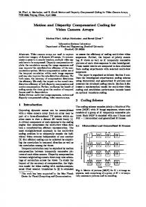
dots with sub-pixel resolution using the hardware anti-aliasing capabilities of the OpenGL board. Half-images for the left and right eyes were presented alternately at a refresh rate of 100 Hz, and stereoscopic presentation was achieved using ferro-electric liquid crystal shutters (DisplayTech) that were synchronized to the video refresh. The RDS consisted of red dots presented on a black background (Fig. 1) to minimize stereo crosstalk between the two eyes (crosstalk was ⬍3%). Note that the 100-Hz refresh rate (50-Hz refresh for each eye) limited the speeds of motion that we could present. A maximal speed of 32°/s was chosen because motion was still quite smooth at this speed. Importantly, the position of each dot in a moving stimulus was updated every video frame with an appropriate compensation for the fact that left and right halfimages were presented on alternate frames. Thus we assured that the binocular disparity of the stimulus was accurate for each direction and speed of motion. Monkeys viewed the random-dot stimuli while maintaining fixation on a small yellow spot (0.15°). The fixation window was typically 1.5° wide. Stimuli were presented for a period of 1.5 s, and monkeys received a liquid reward for maintaining fixation throughout this period (see Fig. 1). If the monkey’s conjugate eye position left the fixation window during the trial, the visual stimulus was terminated, data were discarded, and the monkey was not rewarded. Monkeys were also trained to maintain their vergence angle to within ⫾0.25° of the plane of fixation. A background of stationary dots presented at zero disparity helped to anchor vergence (Fig. 1). After the initial training, we found that all three monkeys accurately maintained their vergence posture as the disparity of the RDS was varied over the neuron’s receptive field. In most recording sessions, a vergence criterion was not enforced, but vergence data were always collected and factored into the analysis of disparity tuning curves (see following text).

Recording procedures and data acquisition METHODS

Experiments were performed on three male rhesus monkeys (Macaca mulatta) weighing 5–7 kg. All experimental procedures were approved by the Institutional Animal Care and Use Committee at Washington University and conformed to National Institutes of Health guidelines.

Tungsten microelectrodes (FHC) were introduced into the cortex through a transdural guide tube and typically passed through extrastriate visual areas in the anterior bank of the lunate sulcus prior to entering area MT. MT was recognized based on extensive experience

Surgical preparation Standard surgical procedures were used to prepare animals for daily training and recording sessions (see Britten et al. 1992; DeAngelis and Newsome 1999 for details). Briefly, a post for head restraint and a recording chamber were affixed to the skull using a combination of titanium screws and cranio-plastic cement (Plastics One). The recording chamber was beveled at an angle of 32 or 36° and centered over occipital cortex at a location roughly 17 mm lateral and 14 mm dorsal to the occipital ridge. An eye coil was implanted under the conjunctiva in each eye, allowing us to monitor both conjugate eye position and vergence angle. To reduce coil slippage and deformation in the eye, each eye coil was sutured to the sclera at three to four locations using either a permanent (8-0 Nylon) or long-lasting dissolvable (7-0 Dexon) suture.

Visual stimuli and task Random-dot stereograms (RDSs) were generated by an OpenGL accelerator board (3Dlabs Oxygen GVX1) and presented on a flatfaced 22-in color display (Sony GDM-F500) subtending 40 ⫻ 30° at a viewing distance of 57 cm. Dot density was 64 dots per square degree per second, each dot subtended ⬃0.1°, and the starting position of each dot within the receptive field was newly randomized for each trial. Precise disparities and smooth motion were achieved by plotting J Neurophysiol • VOL

FIG. 1. Schematic illustration of the visual stimulus used in this study. The display, which subtended 40 ⫻ 30° of visual angle, consisted of red dots presented on a black background. A circular patch of moving dots having variable disparity was presented over the receptive field (dashed circle, not present in the actual display) of a middle temporal (MT) neuron. The remainder of the screen was filled with stationary dots presented with 0 disparity. A small yellow square (0.15 ⫻ 0.15°) served as a fixation point. During each trial, the fixation point and background dots first appeared. After the monkey achieved fixation, moving dots within the receptive field appeared for 1.5 s, after which a liquid reward was delivered if fixation was maintained throughout the trial.

89 • FEBRUARY 2003 •

www.jn.org

1096

G. C. DEANGELIS AND T. UKA

interpreting the patterns of gray and white matter transitions along electrode penetrations, the response properties of single units and multi-unit clusters (direction, speed, and disparity tuning), the relationship between receptive field size and eccentricity, topography within MT, and the subsequent entry into gray matter with response properties typical of area MST. All data included in this study were derived from recordings taken in stretches of gray matter that were confidently assigned to area MT. Behavioral control and data acquisition were accomplished using a commercially available software package (TEMPO, Reflective Computing). Raw neural signals were amplified, band-pass filtered (500 to 5,000 Hz), and discriminated using conventional electronic equipment (Bak Electronics). Only well-isolated action potentials were counted as single-unit responses. Times of occurrence of spikes, along with behavioral event markers, were stored to disk with 1-ms resolution. Horizontal and vertical eye position signals from each eye were sampled at 1 kHz and stored to disk at a rate of 250 Hz. In most experiments, the raw analog signal from the electrode was digitized at 25 kHz and streamed to hard disk using Spike2 software (Cambridge Electronic Design).

Experimental protocol After the action potential of an MT neuron was isolated using a dual voltage-time window discriminator (Bak Electronics), we explored the receptive field and tuning properties of the neuron using a receptive-field mapping program. A small patch (typically 1–3°) of moving or flickering dots was moved around the screen using a mouse, and instantaneous firing rate was plotted on a graphical user interface. This allowed us to carefully center the stimulus over the receptive field and adjust the size of the stimulus to be optimal. Next, we estimated the neuron’s preferred velocity of motion by searching through a polar representation of direction and speed. Finally, we adjusted the horizontal disparity of an optimized patch of moving dots to achieve the largest response from the neuron. After these qualitative tests, four quantitative measurements were taken for each neuron in our sample: a direction tuning curve, a speed tuning curve, a size tuning (area summation) curve, and a disparity tuning curve. Each of these measurements was performed in a separate block of randomly interleaved trials, with each unique stimulus presented three to seven times (typically 5). In all cases, a circular aperture of moving dots was centered on the MT receptive field, and the remainder of the screen was filled with stationary dots having zero disparity to help anchor vergence in the plane of fixation (Fig. 1). Direction tuning was measured by presenting random-dot patterns that drifted in eight different directions, 45° apart. For the occasional narrowly tuned cell, the spacing between directions was reduced appropriately and the test was repeated. Speed tuning was measured (at the preferred direction) by presenting dot patterns that drifted at 0, 0.5, 1, 2, 4, 8, 16, and 32°/s. Next, a size-tuning (area summation) curve was obtained by presenting dots within circular apertures of the following diameters: 0, 1, 2, 4, 8, 16, and 32°. Note that large stimulus patches would often overlap the fixation point, which could elicit tracking eye movements or changes in vergence posture. To avoid this, a small (2° diam) patch of stationary zero-disparity dots always surrounded the fixation point in the size tuning run. Finally, we measured a disparity-tuning curve at the optimal stimulus direction, speed, and size. In most cases, horizontal disparities were tested from ⫺1.6 to 1.6° in steps of 0.4°; however, these parameters were adjusted as necessary based on our initial qualitative assessment of the breadth of disparity tuning.

Data analyses The response of the neuron for each trial was computed as the mean firing rate over the 1.5-s stimulus duration. Tuning curves were constructed by plotting the mean response (across repetitions) to each J Neurophysiol • VOL

stimulus along with the SE of the mean (see Fig. 2). The timeaveraged position of each eye was also computed for each trial, and the horizontal vergence angle was computed as the left eye position minus the right eye position. Averaged across all experiments, the inter-trial variations in (time-averaged) vergence angle had a SD of 0.10°. By comparison, the average within-trial SD of vergence angle was 0.06°. This greater variance of vergence angle across trials versus within trials presumably reflects a small amount of eye-coil slippage or distortion that occurs from trial to trial. Each tuning curve was fit with a function that was chosen because it describes the data well with a relatively small number of parameters. The best fit of each function was achieved by minimizing the sumsquared error between the responses of the neuron and the values of the function, using the constrained minimization tool, “fmincon,” in Matlab (Mathworks). We fit all of the single-trial responses for each stimulus condition not just the mean response. Although this generally yields the same result as fitting the mean response to each different stimulus, fitting all of the single-trial responses allows us to test the goodness-of-fit by comparing residuals around the mean response with residuals around the value of the fitted curve (␹2 goodness-of-fit test, discussed further in the following text). To homogenize the variance of the neural responses across different stimulus values, we minimized the difference between the square root of the neural responses and the square root of the function (see Prince et al. 2002b). Table 1 gives the equations for the functions fit to each tuning curve along with a description of the free parameters. Because neuronal responses must be positive, all fitted curves were half-wave rectified,

FIG. 2. A complete data set for an example MT neuron. In each panel, the mean response (⫾SE) is plotted as a function of the relevant stimulus variable. Each data point (●) is the mean of 5 stimulus repetitions. - - -, the average spontaneous activity level when no stimulus was presented within the receptive field. This neuron’s receptive field was centered 1.4° to the left of and 3.9° below the fixation point. A: direction tuning curve. —, the best-fitting Gaussian (R2 ⫽ 0.971). Discrimination and modulation indices were 0.73 and 0.97, respectively. B: speed tuning curve. —, the best fit of a Gamma distribution (R2 ⫽ 0.968). Discrimination index ⫽ 0.81, modulation index ⫽ 1.09. C: size tuning (area summation) curve. —, the best-fitting difference-of-error functions (R2 ⫽ 0.968). The optimal size is 7.9°, and percentage of surround inhibition is 39%. D: disparity tuning curve. The best-fitting Gabor function is shown by the solid curve (R2 ⫽ 0.932). Discrimination index ⫽ 0.74, modulation index ⫽ 0.91. Points labeled L, R, and U denote response levels obtained for: monocular stimulation of the left eye, monocular stimulation of the right eye, and binocular stimulation with an uncorrelated stereogram, respectively. All curve fits in this figure passed the ␹2 goodness-of-fit test (P ⬎ 0.05).


www.jn.org

DISPARITY CODING IN MACAQUE AREA MT TABLE

1097

1. Equations for curve fits and summary statistics Fitting Equation

Direction tuning

Speed tuning

Size tuning

Disparity tuning

R(␪) ⫽ R0 ⫹ A ⫻ e

R共s兲 ⫽ R0 ⫹ A ⫻

Free Parameters

⫺0.5((␪⫺␪0)2/␴2)

R0 ⫽ baseline response A ⫽ amplitude ␪0 ⫽ preferred direction ␴ ⫽ Gaussian width R0 ⫽ baseline response A ⫽ amplitude ␣ ⫽ scaling factor ␶ ⫽ offset n ⫽ exponent R0 ⫽ baseline response Ae ⫽ excitation amplitude ␣ ⫽ excitation size Ai ⫽ inhibition amplitude ␣ ⫹ ␤ ⫽ inhibition size R0 ⫽ baseline response A ⫽ amplitude d0 ⫽ Gaussian center ␴ ⫽ Gaussian width f ⫽ disparity frequency ⌽ ⫽ phase

共␣共s ⫺ ␶兲兲n ⫻ e⫺共␣共s⫺␶兲兲 nn ⫻ e⫺n

R(w) ⫽ R0 ⫹ Ae ⫻ erf(w/␣) —or— R(w) ⫽ R0 ⫹ Ae ⫻ erf(w/␣) ⫺ Ai ⫻ erf(w/(␣ ⫹ ␤)) (erf denotes the error function) 2

2

R(d) ⫽ R0 ⫹ A ⫻ e⫺0.5((d⫺d0) /␴ ) ⫻ cos(2␲f(d ⫺ d0) ⫹ ⌽)

though this was seldom necessary. The amplitude parameter, A, of each fit was constrained to be no larger than 1.5 times the difference between the maximum and minimum responses. Direction tuning curves were fit with a Gaussian, and speed tuning curves were fit with a Gamma distribution. The choice of a Gamma distribution was simply motivated by the variety of shapes of speed tuning curves that we observed empirically; there was no theoretical basis for this choice. The denominator term in the Gamma formulation normalizes the curve to have an amplitude specified by A. Size-tuning curves were fit with two functions: a single error function (erf, the integral of a Gaussian) and a difference of error (DoE) functions. The single error function provided good fits to size tuning curves for neurons that lacked surround inhibition, whereas the DoE function was necessary for neurons with surround inhibition (e.g., Fig. 2C). The errors of these two fits were compared for each neuron using a sequential F test (Draper and Smith 1966). If the DoE function provided a significantly better fit than the single error function (P ⬍ 0.05), the neuron was considered to have significant surround inhibition and the optimal stimulus size was taken as the peak of the DoE fit. Otherwise, the optimal size was taken from the single error function as 1.163␣, which defines the size at which the curve reaches 90% of its maximal value. Disparity tuning curves were fit with a Gabor function, as done previously for V1 neurons (e.g., Ohzawa et al. 1997; Prince et al. 2002b). Because the disparity frequency, f, is often poorly constrained by the data at the low-frequency end of the spectrum, this parameter was only allowed to vary within ⫾10% of the peak frequency determined from a Fourier transform of the raw tuning curve (after subtracting the DC response). We found that this constraint considerably improved the convergence of the optimization (see also Prince et al. 2002b) with minimal increase in the overall error of the fits. We also constrained the center of the Gaussian component, d0, to lie within the range of disparities that was tested. To test whether the six-parameter Gabor function was necessary to fit our disparity tuning curves, we also fit each curve separately with both a Gaussian and a sinusoid. Results of these comparisons will be discussed later. The functions described in Table 1 generally provided excellent fits to the tuning curves of MT neurons as evidenced by the median R2 values given for each function. We also tested the quality of the fits by performing a ␹2 goodness-of-fit test on each data set with significant tuning (ANOVA, P ⬍ 0.05). This is a rather stringent test that assesses whether the residuals around the values of the fitted curve have a significantly larger variance than the residuals around the mean responses. As seen in Table 1, 64 – 81% of MT neurons pass this test J Neurophysiol • VOL

Fit Statistics Median R2 ⫽ 0.967 310/488 pass ␹2 test (P ⬎ 0.05) Median R2 ⫽ 0.979 400/496 pass ␹2 test (P ⬎ 0.05) Median R2 ⫽ 0.977 343/493 pass ␹2 test (P ⬎ 0.05) Median R2 ⫽ 0.939 379/471 pass ␹2 test (P ⬎ 0.05)

for the different tuning functions, indicating that most of the fits were very good. Moreover, most of the neurons that failed the ␹2 test still had R2 values in excess of 0.9. None of our population analyses differed when these neurons were removed from the sample, thus we did not exclude neurons from study based on the ␹2 test alone. From each direction, speed, and disparity tuning curve, we extracted two different measures of tuning strength. A modulation index characterized the amount of response modulation due to stimulus variations, relative to the maximal response Modulation Index ⫽

Rmax ⫺ Rmin Rmax ⫺ S

(1)

where Rmax and Rmin are the mean responses to the most effective and least effective stimuli, respectively, and S denotes the spontaneous activity level of the neuron. Note that this index does not consider response variability; hence, a neuron with weak, noisy responses could show a spuriously high value of this index. We therefore also computed a discrimination index (Prince et al. 2002b), which characterizes the ability of a neuron to discriminate changes in the stimulus relative to its intrinsic level of variability Discrimination Index ⫽

Rmax ⫺ Rmin

Rmax ⫺ Rmin ⫹ 2 冑SSE/共N ⫺ M兲

(2)

where SSE is the sum squared error around the mean responses, N is the number of observations (trials), and M is the number of stimulus values (e.g., directions or speeds) tested. Both the modulation and discrimination indices were computed from the square root of the firing rate. For each size-tuning curve, we computed the percentage of surround inhibition as % Surround Inhibition ⫽ 100 ⫻

冉

冊

Ropt ⫺ Rlargest Ropt ⫺ S

(3)

where Ropt is the response at the optimal size (determined from the curve fit), Rlargest is the response to the largest size, and S denotes the spontaneous activity level. This metric was always computed from the DoE fit, and its significance was assessed using the sequential F test, as described in the preceding text. The preferred direction, speed, and disparity for each neuron were given by the value at which the fitted curves reached a peak.


www.jn.org

1098


Population statistical analyses Our data set consisted of single-unit recordings from three different monkeys. Because differences in the distribution of parameters among monkeys could produce misleading results in correlation analyses, all such analyses were done using a within-cells regression in the context of an analysis of covariance (ANCOVA), with monkey identity as an independent factor. Thus all correlation coefficients and P values reported here are corrected for differences between subjects. RESULTS

Neuronal database The sample for this study consists of 501 MT neurons that were recorded from three monkeys (230 units from monkey B, 166 from monkey J, and 105 from monkey R). For each of these neurons, we obtained a complete set of data consisting of a direction tuning curve, a speed tuning curve, a size tuning (area summation) curve, and a horizontal disparity tuning curve. An example data set for one of the MT units is shown in Fig. 2. The smooth curves (—) fitted to the data in Fig. 2 are described by the equations given in Table 1. This example neuron had broad direction tuning, preferred far dots moving at slow speeds and exhibited substantial surround inhibition. This example was chosen for illustration because the R2 values of the fits were average or slightly below average (compare with median values in Table 1). Thus this neuron is truly representative of the quality of the curve fits that we obtained for most MT neurons. Figure 3A shows a polar representation of the preferred directions and speeds for 481/501 MT neurons that had significant tuning for both direction and speed of motion. It is clear that the population represents all directions of motion across a broad range of speeds. Figure 3B presents a summary of the size-tuning properties in which the percentage of surround inhibition is plotted against the optimal stimulus size. Surround inhibition was statistically significant for 42% of MT neurons (P ⬍ 0.05, sequential F test, see METHODS), with surround inhibition in excess of 20% generally reaching statistical significance (F). These data are roughly compatible with previous results from MT (e.g., Born 2000; Raiguel et al. 1995). Together, the data of Fig. 3 show that we sampled MT neurons with a broad range of stimulus preferences. Most of the cells in our sample were significantly tuned (ANOVA, P ⬍ 0.05) for direction of motion (96%), speed of motion (99%), and horizontal disparity (93%). As our percentage of disparity-selective neurons was higher than the 68% reported by Maunsell and Van Essen (1983c) in the anesthetized monkey, we worried that eye movements could be a factor. We thus performed an analysis of covariance on the responses of each neuron with disparity as the independent factor and vergence angle as a covariate. Only 59/501 (11%) MT neurons exhibited a significant correlation between response and vergence angle (ANCOVA within-cells regression, P ⬍ 0.05), and the significance of the main effect of disparity was unchanged for all but 15 neurons when vergence angle was included as a covariate in the analysis. Thus vergence posture was under reasonably tight control, and small variations in vergence angle from trial to trial did not have a significant impact on our disparity tuning curves. The lower percentage of disparity-selective neurons reported by Maunsell and Van EsJ Neurophysiol • VOL

FIG. 3. Direction, speed, and size preferences of the MT population. A: a polar plot is shown in which the angular variable is the preferred direction of motion, and the radial variable is the preferred speed of motion. Data are presented for 481/501 MT neurons with significant tuning for both direction and speed of motion. Note that MT neurons cover this space almost uniformly. B: the percentage of surround inhibition is plotted as a function of the optimal stimulus size for each MT neuron. These parameters were derived from the size-tuning curve for each neuron (see METHODS). ●, MT neurons for which surround inhibition was statistically significant (sequential F test, P ⬍ 0.05, see METHODS).

sen (1983c) may reflect a different criterion for significance, which is not stated in their study. We assessed the strength of tuning for direction, speed, and disparity using both a modulation index (Eq. 1) and a discrimination index (Eq. 2). Figure 4A shows the distribution of the modulation index for direction, speed, and disparity tuning measurements across the population of MT neurons. As numerous studies have shown previously (e.g., Albright 1984; Britten et al. 1992; Maunsell and Van Essen 1983b; Mikami et al. 1986; Snowden et al. 1992), the distribution of modulation indices for direction tuning (䡲 in Fig. 4A) is centered at ⬃1.0 (mean ⫽ 0.97), indicating that the difference in response between the preferred and null directions is typically equal to the difference between the preferred response and the spontaneous activity level. The distribution of modulation indices for speed tuning (u) is similarly distributed around ⬃1.0, and the mean modulation index for speed (0.96) is not significantly different from that for direction (paired t-test, P ⫽ 0.21). In contrast to direction and speed, the modulation indices for horizontal disparity tuning are not distributed around 1.0; rather the mean modulation index (0.73) is significantly lower than that for direction or speed (paired t-test, P ⬍⬍ 0.0001 for both comparisons). Thus although 93% of MT neurons are significantly tuned for disparity, the response modulations elic-


www.jn.org


1099

having a continuous range of disparity preferences and shapes rather than forming discrete classes. As Prince et al. (2002a) reported for V1, we see no evidence that disparity-tuning curves in MT form discrete classes. The smooth curves (—) in Fig. 5 are the best-fitting Gabor functions for each neuron. Table 2 gives the parameters of the fits, as well as other relevant information, for each of these example units. To facilitate interpretation of Gabor fits here and throughout the paper, Fig. 6 shows a graphic depiction of each of the six parameters of the Gabor function. Note, in particular, that the phase of the sinusoidal component is specified relative to the center of the Gaussian envelope (Fig. 6B), such that neurons with phases of 0 and 90° have even- and odd-symmetric curves, respectively. As discussed in the preceding text, Gabor functions provide an excellent description of the data for ⬃80% of MT neurons (␹2 test, Table 1). However, the question arises as to whether

FIG. 4. Comparison of tuning indices for direction, speed, and horizontal disparity across the population of 501 MT neurons. A: distributions of the modulation index, as defined by Eq. 1. ■, 1, and o, distributions for direction, speed, and disparity tuning, respectively. B: distributions of the discrimination index, as defined by Eq. 2.

ited by varying disparity are somewhat smaller than those elicited by varying direction or speed. A similar pattern of results is observed for the discrimination index (Fig. 4B), which takes into account the variability of responses across repetitions of a given stimulus. The median discrimination indices for direction (0.819) and speed (0.818) are indistinguishable (sign test, P ⬎ 0.5), whereas the median disparity discrimination index (0.74) is significantly lower (sign test, P ⬍⬍ 0.0001 for both comparisons). Thus individual MT neurons tend to have slightly lower discriminative capacity for horizontal disparity than for direction or speed of motion. Quantitative description of disparity tuning curves of MT neurons We now consider the variety of disparity tuning in MT and describe methods for parametric characterization of disparity tuning curves. MT neurons have preferred disparities that cover a large range of crossed and uncrossed disparities. Figure 5 shows disparity tuning curves (along with Gabor fits) for 13 MT neurons that typify the variety of responses that we see across the population. Some of these neurons could be described as near (units 1 and 2) or far (units 11 and 12) cells in the terminology used by Poggio and colleagues (1988). Units 6 and 7 could be described as tuned-zero cells, whereas the remaining neurons would be classified as tuned-near (units 3–5), tuned-far (units 8 –10), or tuned inhibitory (unit 13). Alternatively, the 13 units in Fig. 5 could well be described as J Neurophysiol • VOL

FIG. 5. Disparity tuning curves for 13 representative MT neurons. ●, the mean response to each disparity ⫾SE. —, the best-fitting Gabor function. Neurons 1–12 are presented (from top to bottom) in order of their preferred disparities, from large near to large far. The vertical scale bar corresponds to 100 spikes/s.


www.jn.org

1100 TABLE


2. Receptive field and curve-fit parameters for the example neurons in Fig. 5

Cell No.

PDir, °

PSpd, °/s

Ecc, °

Mod Index

Disc Index

Rmax, spikes/s

Dmax, °

Ro, spikes/s

A, spikes/s

d0, °

␴, °

f, cycle/°

⌽, °

R2

1 2 3 4 5 6 7 8 9 10 11 12 13

141 231 260 202 138 160 85 139 269 227 317 261 198

12.9 15.9 1.2 4.5 7.1 6.5 3.2 2.8 1.2 6.7 26 32 4.4

14.1 3.1 10.0 6.2 5.4 3.3 9.9 7.1 10.2 6.7 8.4 24.7 6.2

0.66 0.77 0.94 0.85 0.85 0.93 0.94 0.94 0.97 1.03 0.91 0.69 1.17

0.81 0.79 0.82 0.81 0.88 0.87 0.86 0.81 0.86 0.92 0.82 0.74 0.85

110 128 125 75 178 126 72 122 93 108 64 63 116

⫺1.12 ⫺1.20 ⫺0.81 ⫺0.46 ⫺0.2 ⫺0.02 0.16 0.29 0.39 0.53 0.98 1.12 0.68

72 77 81 41 75 32 24 51 59 18 16 33 101

44 67 73 42 110 124 51 77 46 121 49 31 92

⫺0.23 ⫺0.46 0.15 ⫺0.11 ⫺0.04 ⫺0.16 ⫺0.02 0.04 ⫺0.01 0.24 0.81 1.6 ⫺0.23

1.86 1.16 1.07 0.62 0.53 0.31 0.62 0.67 0.57 0.52 1.01 2.10 0.56

0.19 0.25 0.28 0.43 0.51 0.37 0.42 0.50 0.49 0.30 0.21 0.19 0.33

74 86 123 73 40 ⫺51 ⫺38 ⫺55 ⫺92 ⫺61 ⫺19 38 ⫺162

0.98 0.99 0.99 0.99 0.98 0.99 0.97 0.98 0.99 0.99 0.95 0.99 0.98

PDir, preferred direction; PSpd, preferred speed; Ecc, eccentricity; Mod Index, disparity modulation index; Disc Index, disparity discrimination index; Rmax, response at preferred disparity; Dmax, preferred disparity; Ro, Gabor baseline level; A, Gabor amplitude; do, Gabor center; ␴, Gabor width; f, Gabor frequency; ⌽, Gabor phase; R2, proportion of variance accounted for by Gabor fit.

a six-parameter Gabor function is necessary to describe these data. To address this question, we also fit each disparity-tuning curve with a Gaussian and a sinusoid (the 2 components of a Gabor function), and we compared the quality of the fits statistically using a sequential F test (Draper and Smith 1966).

FIG. 6. Graphical illustration of the components and parameters of the Gabor function used to fit disparity tuning curves. A: ●, disparity tuning data for an MT neuron; —, the best-fitting Gabor function; - - -, the Gaussian envelope of the Gabor fit. R0 indicates the baseline response parameter, and A gives the amplitude of the Gabor function (height of the Gaussian envelope). B: the Gaussian (bottom) and sinusoidal (top) components of the Gabor function are shown separately here. The half-width of the Gaussian envelope is given by ␴, and the center location of the Gaussian envelope on the disparity axis is given by d0. The frequency of the sinusoid is f (1/f is the period), and ␾ gives the phase of the sinusoid relative to the center of the Gaussian envelope.

J Neurophysiol • VOL

Figure 7A shows the R2 value of the Gabor fit plotted against the R2 value for the sinusoidal fit; one data point is shown for each of 471 MT neurons that had significant disparity tuning (ANOVA, P ⬍ 0.05). In most cases, the Gabor function accounted for substantially more of the variance in the data than the sinusoid, and the Gabor function provided a significantly better fit for 313/471 neurons (F; sequential F test, P ⬍ 0.05). Figure 7B shows the analogous comparison between Gabor fits and Gaussian fits; 202/471 tuning curves were significantly better fit by a Gabor function. These comparisons show that many MT tuning curves can be well fit by either the Gaussian or sinusoidal component of the Gabor function and do not require both. Thus in a later section when we analyze the position and phase components of the disparity tuning curve, we shall focus on a subset of 185 neurons for which the Gabor fit was significantly better than both the Gaussian and sinusoidal fits. It is important to note that there are a number of factors that affect the relative quality of the Gabor, Gaussian, and sinusoidal fits. For example, units 1 and 3 of Fig. 5 may have been well fit by a sinusoid because we did not test a wide enough range of disparities to observe the response plateau at large disparities. In fact, it seems likely that many of the 158 neurons that were well fit by a sinusoid would have been better fit with a Gabor function over a larger disparity range. This explanation does not account for most of the cells that were adequately fit with a Gaussian, however. Many of these cells simply lacked clear side lobes in their disparity tuning curves (e.g., units 6 and 13 of Fig. 5) or had shallow side lobes that were clipped off because the response to uncorrelated dots (and consequently the baseline level of the Gabor function) was rather low (e.g., unit 10 of Fig. 5). Gabor fits for these cells might have been superior if the responses were averaged across more repetitions of each stimulus. Thus our estimates of the proportion of MT cells that require a Gabor fit is probably quite conservative. Population analyses and comparisons to other visual areas When comparing our results to disparity-tuning data from other areas, it is important to consider the range of receptive field eccentricities studied. For example, most studies of dis-


www.jn.org


1101

phase of the Gabor function plotted against eccentricity. Positive values of the Gabor phase denote phase shifts that move the peak of the Gabor function toward Near disparities (e.g., units 3–5 of Fig. 5). The distribution of Gabor phases is clearly bimodal, such that there are many MT neurons with tuning curves close to odd-symmetric (phases near ⫾␲/2), whereas relatively few MT neurons have even-symmetric tuning curves (phases near 0 and ⫾␲). This pattern contrasts with that seen in V1, where there is a preponderance of even symmetry (Cumming and DeAngelis 2001; Prince et al. 2002a). This difference between areas is not due to different ranges of eccentricities because the bimodal pattern of spatial phases is seen for MT neurons at all eccentricities tested. It is notable, and perhaps somewhat confusing, that the distribution of preferred disparities in Fig. 8A is unimodal,

FIG. 7. Comparison of the variance accounted for by Gabor, Gaussian, and sinusoidal fits to disparity tuning functions. Each R2 value was obtained by regressing the mean response of the neuron against the value of the best-fitting function. Neurons lacking significant disparity tuning were excluded from this analysis. A: the R2 value for the Gabor fit is plotted against R2 for the sinusoidal fit. ●, neurons for which the Gabor function provides a significantly better fit than the sinusoid (sequential F test, P ⬍ 0.05). Arrow heads inside the axes show the median values of R2 for each type of fit. B: R2 for Gabor fits is plotted against R2 for Gaussian fits, using the same conventions as in A.

parity tuning in primate V1 have focused on the central 5° of the visual field (e.g., Poggio et al. 1988; Prince et al. 2002b), whereas previous studies in MT have generally focused on larger eccentricities (Maunsell and Van Essen 1983c; DeAngelis and Newsome 1999). Figure 8 shows how a few key parameters of disparity tuning in MT vary with receptive field eccentricity. Figure 8A shows the preferred disparity of each neuron with significant disparity tuning (ANOVA, P ⬍ 0.05) as a function of eccentricity. As others have reported (Bradley and Andersen 1998; Maunsell and Van Essen 1983c), there are more MT neurons tuned to near than far disparities, and this tendency is maintained across the range of eccentricities tested. The mean preferred disparity across the sample is ⫺0.22, which is significantly less than zero (t-test, P ⬍⬍ 0.0001). There is a weak positive correlation between the magnitude of the preferred disparity and eccentricity (R ⫽ 0.09, P ⫽ 0.048). Figure 8B shows how the disparity frequency, which is a measure of the coarseness of disparity tuning, varies with eccentricity. There is a highly significant negative correlation in this plot (R ⫽ ⫺0.20, P ⬍⬍ 0.0001) as expected if the spatial scale of disparity selectivity increases along with receptive field size at large eccentricities. Finally, Fig. 8C shows the J Neurophysiol • VOL

FIG. 8. Distributions of 3 disparity-tuning parameters as a function of eccentricity for 471 MT neurons with significant tuning. ●, ■, and Œ, data for the 3 different monkeys. Histograms along the right margin show the same data collapsed along the eccentricity axis. A: preferred disparity, defined as the disparity at which the best-fitting Gabor function peaks. B: disparity frequency. C: phase of the best-fitting Gabor function in radians. Positive values correspond to phases that shift the peak of the tuning curve toward near (crossed) disparities.


www.jn.org

1102


whereas the distribution of Gabor phases (Fig. 8C) is bimodal. This indicates that some other parameter of the Gabor function must counterbalance the phase to distribute the preferred disparities unimodally. We shall see later (Fig. 15) that the position parameter (d0) of the Gabor function accounts for this apparent inconsistency. We now compare our results from MT with some recently published data from areas V1 and V4. Figure 9A shows distributions of the disparity discrimination index (DDI) for MT, V1 (data from Prince et al. 2002b), and V4 (data from Watanabe et al. 2002). Although all three distributions overlap considerably, it is quite clear that the average MT neuron is more sensitive to disparity than the average V1 or V4 neuron. The median values of DDI are 0.74 for MT, 0.54 for V1, and 0.50 for V4. Note that the most sensitive neurons in V1 and (to a lesser extent) V4 are comparable to the most sensitive MT neurons. However, relatively few V1 and V4 neurons have DDI values ⬎0.7, whereas the majority of MT neurons exceed this criterion. It should be noted that there are considerable stimulus differences between the V4 study and ours. Responses of MT neurons were generally well sustained throughout the entire 1.5-s stimulus period. In contrast, Watanabe et al. (2002) measured responses to stationary bar stimuli presented for 1s, and their responses were generally much more transient than ours. To gauge how much these differences affect the comparison of Fig. 9A, we recomputed DDI values for our MT

neurons based on the first 300 ms of responses following stimulus onset. The median DDI for MT declined by 14% from 0.74 to 0.64, but is still substantially larger than that seen for V4. Thus it seems clear that MT neurons are generally more sensitive to horizontal disparity than neurons in V1 and V4. This difference in disparity sensitivity between areas is unlikely to be the result of differences in the range of eccentricities tested because we found no significant dependence of DDI on eccentricity for our sample of MT neurons (R ⫽ 0.05, P ⫽ 0.28). Another possible explanation for the difference between V1 and MT in Fig. 9A is that the V1 neurons were tested with dynamic random-dot stereograms in which dots were randomly replotted every few video frames, whereas our MT neurons were tested with stereograms containing dots moving coherently in the preferred direction. We have tested a handful of MT neurons with moving and dynamic stereograms and have found DDI values to be very similar for the two types of stimuli, but our sample is not large enough for a rigorous statistical analysis. Nevertheless, this factor seems unlikely to account for the large difference in DDI values between MT and V1. Although responses of MT neurons are more strongly modulated by disparity than responses of V1 neurons, Fig. 9B shows that MT neurons are more broadly tuned. Disparity frequency is plotted against eccentricity for populations of V1 neurons recorded by Prince et al. (2002b) and B. G. Cumming (unpublished results), along with our MT data. Over the range of eccentricities from 2 to 8°, where the data overlap, the median disparity frequency for V1 (0.89) is significantly higher than the median value (0.30) for MT (Mann-Whitney U test, P ⬍⬍ 0.0001). This difference is confirmed by an analysis of covariance on the entire data set, which reveals a highly significant difference between areas (P ⬍⬍ 0.0001) as well as a significant dependence on (log) eccentricity (partial R ⫽ ⫺0.30, P ⬍⬍ 0.0001). MT neurons are clearly more broadly tuned for disparity than V1 neurons at comparable eccentricities. There is a somewhat abrupt falloff in the number of MT neurons with disparity frequencies below ⬃0.2 cycles/° (see histogram in Fig. 8B). Because the disparity frequency of the Gabor fit was constrained using the Fourier transform of the disparity tuning data (see METHODS), the range of disparities tested imposes a lower bound on the disparity frequency estimate. Thus some broadly tuned neurons would have a lower disparity frequency if a wider range of disparities were tested. Note, however, that any errors introduced by the limited disparity range are in the wrong direction to account for the difference in disparity frequency between V1 and MT. Relationships between disparity tuning and velocity tuning in MT

FIG.

9. Comparison of disparity selectivity in areas MT, V1, and V4. A: the distribution of the disparity discrimination index (DDI) is shown for our sample of 501 MT neurons (■) as well as for 789 V1 neurons tested by Prince et al. (2002b) (䊐) and 121 V4 neurons studied by Watanabe et al. (2002) (o). B: disparity frequency is plotted against eccentricity for V1 and MT. The V1 data (E and ‚) are taken from the study of Prince et al. (2002a) (‚) as well as an unpublished study by B. G. Cumming (E). ●, data for our sample of 471 MT units with significant disparity tuning. Note that, in the range of eccentricities where the MT and V1 samples overlap, disparity frequencies are substantially higher for V1 neurons. J Neurophysiol • VOL

To understand population coding of disparity and velocity in MT, it is of considerable interest to know how disparity tuning correlates with the other response properties of MT neurons, namely direction, speed, and size tuning. We thus performed a series of multiple regression analyses with the following parameters as independent variables: direction discrimination index, preferred direction, direction tuning width, speed discrimination index, preferred speed, optimal size, percentage of surround inhibition, eccentricity, and monkey identity. Be-


www.jn.org


1103

ously reported by DeAngelis and Newsome (1999) based on multi-unit recordings in MT. The lack of any significant correlation between DDI and direction tuning parameters is also noteworthy and is consistent with findings of the previous multiunit study as well. We also examined the dependence of disparity frequency on other tuning parameters. Figure 11A shows that disparity frequency depends on the preferred speed of MT neurons, such that neurons preferring fast speeds tend to have lower disparity frequencies (partial R ⫽ ⫺0.25, P ⬍ 0.0001). This relationship is sensible if the disparity frequency of MT neurons is correlated with their monocular spatial frequency preferences as is the case in V1 (Ohzawa et al. 1997; Prince et al. 2002b). Neurons that prefer low spatial frequencies would be expected to have faster speed preferences, given that velocity is inversely proportional to spatial frequency in the Fourier domain. Disparity frequency is not significantly correlated with direction or size tuning parameters. Figure 11B shows that disparity frequency is negatively correlated with the absolute value of the preferred disparity (partial R ⫽ ⫺0.53, P ⬍⬍ 0.0001), indicating that neurons with large disparity preferences tend to have broad tuning. This is expected if nonzero disparity preferences are mainly the result of phase shifts in the disparitytuning curve, rather than position shifts. The relative contribu-

FIG. 10. Correlations between disparity selectivity and speed selectivity at the population level. A: the DDI is plotted against the speed discrimination index for each neuron in our sample. B: the DDI is plotted against the preferred speed of each MT neuron.

cause direction is a circular variable, we wrapped preferred directions into the range from 0 to 90°, so that we could test for differences between neurons coding horizontal and vertical directions. Variables were log transformed before analysis whenever this improved the normality of the distributions, and all significant effects reported in the following text were verified using nonparametric statistics separately. Because the data set is large and very small effects can reach marginal significance, we adopted a significance criterion of P ⬍ 0.01. We first examined how the DDI depends on other tuning parameters. Only two variables were significant predictors of DDI: the speed discrimination index and the preferred speed. Figure 10A shows the positive correlation between DDI and speed discrimination index (partial R ⫽ 0.21, P ⫽ 0.00014), indicating that neurons with strong speed tuning also tend to have strong disparity tuning. This effect is not simply due to the fact that the two metrics share a common variability term (see Eq. 2), as a significant correlation is also found between modulation indices for speed and disparity (R ⫽ 0.18, P ⬍ 0.0001). Figure 10B shows that DDI also depends significantly on the preferred speed of MT neurons (partial R ⫽ ⫺0.19, P ⫽ 0.00085), such that neurons preferring fast speeds tend to have weaker disparity selectivity. This confirms the result previJ Neurophysiol • VOL

FIG. 11. Relationships between disparity frequency and other tuning parameters. A: disparity frequency tends to be lower for neurons that prefer faster speeds. B: disparity frequency is inversely related to the magnitude of preferred disparity.


www.jn.org

1104


tions of phase and position components to the disparity preference will be analyzed further in the following text. For a fixed physical speed of an object through the environment, the speed of retinal image motion will be much larger when the object is close to the observer. Thus one might expect to observe a correlation between the preferred speed and preferred disparity of MT neurons. Specifically, the expectation would be that cells preferring near (crossed) disparities might be tuned to faster speeds than cells preferring far (uncrossed) disparities. Moreover, it is possible that this behavior would be specific to neurons with surround inhibition, as these have been proposed to code object motion rather than self-motion (Born and Tootell 1992; Born et al. 2000). To examine this possibility, we performed a two-way factorial ANOVA across the population of neurons with speed preference as the dependent variable. Sign of preferred disparity and significance of surround inhibition were factors. We find no significant tendency for preferred speeds to depend on either the disparity preference (crossed vs. uncrossed) or the presence of surround inhibition (P ⬎ 0.15 for both). There was also no significant correlation between disparity preference and speed preference in a regression analysis. Thus we see no evidence to support the idea that the MT population incorporates the ecological relationship between retinal image speed and object distance. Of course, we might miss such a relationship because we have measured disparity selectivity not distance selectivity. If MT neurons only code retinal disparity (a hypothesis that we are currently testing), then they will be activated by objects at many different distances, depending on the viewing distance. Thus ecological considerations might predict little or no relationship between speed and disparity preferences over the range of speeds that we have tested. It should also be noted that our findings do not rule out the possibility that individual MT neurons show a disparity preference that varies with the speed of the stimulus. Because we did not systematically explore the interactions between disparity and speed for single neurons, we cannot address this possibility rigorously. However, in exploring the stimulus space qualitatively during receptive field mapping, we didn’t noticed any clear interaction between disparity and speed in determining the response of MT neurons.

small percentage of neurons having a strong preference for one eye. Figure 12B plots the contralateral (▫) and ipsilateral (‚) monocular responses against the response obtained with binocularly uncorrelated dots. In general, the monocular responses are about equal to the uncorrelated response. Figure 12B also shows the baseline level of the fitted Gabor function (R0, F) plotted against the response to binocularly uncorrelated dots. As can be seen by the tight clustering around the unity-slope diagonal, these two values are nearly identical for most neurons. Thus the uncorrelated response corresponds to the base-

Relationships between disparity tuning and responses to monocular and uncorrelated stimuli Previous studies have reported links between disparity tuning and the monocular response properties of neurons in V1 and V2 (Ferster 1981; LeVay and Voigt 1988; Poggio and Fischer 1977). We therefore examined how the sensitivity and shape of disparity tuning depends on monocular responses of MT neurons. We computed an ocular dominance index (ODI) as ODI ⫽

RContra RContra ⫹ RIpsi

(4)

where RContra and RIpsi denote responses to random-dot patterns presented monocularly to the contralateral and ipsilateral eyes, respectively. Figure 12A shows the distribution of ODI for our population of MT neurons. As others have reported (Felleman and Kaas 1984; Maunsell and Van Essen 1983c; Zeki 1974b) for anesthetized monkeys, the vast majority of MT neurons are driven almost equally well through the two eyes with only a J Neurophysiol • VOL

FIG. 12. Relationship of disparity tuning to monocular response properties of MT neurons. A: distribution of the ocular dominance index, Eq. 4, for our sample of 501 MT neurons. Note that most neurons are equally driven by the 2 eyes. B: responses to stimulation of the contralateral (䊐) and ipsilateral (‚) eyes are plotted against the response to binocularly uncorrelated dots for each MT neuron. Monocular responses are generally very similar to the uncorrelated response. In addition, the baseline response level of the fitted Gabor function is shown by ●. The values of this parameter were generally very similar to the uncorrelated responses. C: the monocularity index, Eq. 5, is plotted against the phase of the best-fitting Gabor function for 471 neurons with significant disparity tuning. ●, ■, and Œ, data from the 3 monkeys. Neurons with phases between 0 and ⫾␲/4 are considered to be tuned-zero, those with phases between ⫾␲/4 and ⫾3␲/4 are categorized as near and far cells, and units with phases between ⫾3␲/4 and ⫾␲ are considered to be tuned-inhibitory.


www.jn.org


line level around which responses are modulated by crossed and uncrossed disparities. Other studies have reported a correlation between the ocular dominance of cortical neurons and the shape of disparity tuning. Specifically, near and far cells were found to be more monocularly driven than tuned-excitatory cells (Ferster 1981; LeVay and Voigt 1988; Poggio and Fischer 1977; but see Prince et al. 2002a). To examine this relationship for MT, we computed a monocularity index as Monocularity Index ⫽ 2 ⫻ 兩ODI ⫺ 0.5兩

(5)

Figure 12C shows the monocularity index plotted as a function of the Gabor phase for each neuron with significant disparity tuning. Neurons with phases between 0 and ⫾␲/4 can be considered as tuned-excitatory, neurons with phases between ⫾␲/4 and ⫾3␲/4 as near or far, and neurons with phases between ⫾3␲/4 and ⫾␲ as tuned-inhibitory. It is clear from this plot that there is no tendency for near and far cells to be more monocular than tuned-excitatory neurons. In fact, there is a statistically significant negative correlation between monocularity and Gabor phase (R ⫽ ⫺0.13, P ⫽ 0.004), such that tuned-excitatory neurons tend to be slightly more monocular than the other types. Figure 13A shows that the DDI is also significantly correlated with Gabor phase, such that tuned-excitatory neurons

1105

tend to have larger values of DDI than the other types (R ⫽ ⫺0.18, P ⬍ 0.0001). This is not due to differences in response variability among tuning types, as the variability term of the DDI (Eq. 2) is not correlated with Gabor phase (R ⫽ ⫺0.03, P ⫽ 0.55). Rather, the mean responses of tuned-excitatory neurons are more strongly modulated by horizontal disparity, and this pattern can be understood in terms of response modulations around the level of response to binocularly uncorrelated dots. We assessed the positive and negative response variations around this level by computing a facilitation index Facilitation Index ⫽ 1 ⫺

Runcorr ⫺ Rmin Rmax ⫺ Rmin

(6)

where Rmax and Rmin are the peak and trough response levels from the Gabor fit and Runcorr is the response to binocularly uncorrelated dots. If the response of a neuron is modulated symmetrically around Runcorr, the facilitation index will be 0.5. Figure 13B shows that there is a strong negative correlation between the facilitation index and the Gabor phase (R ⫽ ⫺0.56, P ⬍⬍ 0.0001). Neurons with phases near zero (tunedexcitatory) have large values, indicating that response modulation due to disparity variation consists mainly of increased responses above the level of Runcorr, with relatively little suppression below the uncorrelated response. In contrast, for tuned-inhibitory neurons with phases near ⫾␲, the facilitation index is generally close to zero. For these units, response modulations due to disparity consist almost entirely of suppression below the level of the uncorrelated response (e.g., unit 13 in Fig. 5). Because the amount by which responses can be suppressed depends on the level of Runcorr, this limits the range of response modulations that can be exhibited by tuned-inhibitory neurons and accounts for the phase dependence of the DDI (Fig. 13A). A similar result was found by Prince et al. (2002a) in their study of V1 neurons. Phase and position components of disparity tuning in MT

FIG. 13. Dependence of disparity sensitivity on Gabor phase. A: the DDI is plotted against Gabor phase for all MT neurons with significant disparity tuning. B: the facilitation index, Eq. 6, is plotted against Gabor phase. A value of 0.5 on the ordinate indicates that responses of the neuron are modulated symmetrically around the response to binocularly uncorrelated dots. Values near 1 indicate that disparity tuning mainly involves facilitation of responses above the uncorrelated response level; values near 0 mean that disparity tuning is mainly sculpted out of suppression below the uncorrelated response.


Work done over the past decade or so in V1 has revealed that disparity selectivity depends on interocular differences in both the position and phase of monocular receptive fields (Anzai et al. 1997, 1999; DeAngelis et al. 1991, 1995; Ohzawa et al. 1996; Prince et al. 2002a). For V1 simple cells, the phase difference between receptive fields for the two eyes determines the shape (or phase) of the disparity-tuning curve, and the position disparity between the receptive fields shifts the disparity-tuning curve horizontally along the disparity axis (see DeAngelis et al. 1995; Prince et al. 2002a). The parameters of the Gabor fit to a disparity-tuning curve are thus directly related to the position and phase disparities of V1 receptive fields (see Prince et al. 2002b). Clearly, we should not expect any simple relationship between the disparity-tuning curve and the monocular receptive fields of MT neurons because MT receptive fields are much larger than those in V1 and must be the result of a considerable convergence of inputs. Thus the position and phase components of Gabor fits to MT data cannot be simply interpreted in terms of the underlying receptive field structure, as is the case for V1 simple cells. Nevertheless, we shall see that it is useful to analyze the disparity tuning curves of MT neurons in terms of their position and phase components to better understand how the disparity preference of MT neu-


www.jn.org

1106


rons is determined, and to gain some insight into the population coding of disparity in MT (see DISCUSSION). Figure 14 plots the phase of the Gabor function (in radians) against the position of the Gaussian envelope for our population of MT neurons. Neurons for which the disparity tuning curve is significantly better described by a Gabor function than either a Gaussian or sinusoid are denoted (䡲, sequential F-test, P ⬍ 0.05 for both). For these 185 units, both the position and phase parameters of the Gabor fit were well constrained by the data. We therefore analyzed this subset of neurons to examine the position and phase components of disparity tuning. Regarding Fig. 14, it is worth noting that the envelope locations (i.e., position disparities) are distributed evenly around zero disparity, whereas the Gabor phases are bimodally distributed away from zero. This tendency toward odd-symmetry is especially clear for the subset of neurons that require Gabor fits (F). To clarify how phase and position components contribute to the disparity preference of MT neurons, it is useful to convert the Gabor phases into equivalent “phase disparities” (in degrees of visual angle) by dividing the angular phase by the disparity frequency (a sign inversion is also done to give the phase disparities the same sign as the position disparities). Figure 15A shows the preferred disparity of each MT neuron (defined by the peak of the fitted Gabor function) plotted against the phase disparity in degrees of visual angle. The vast majority of data points lie in the top-right and bottom-left quadrants, indicating that the sign of the phase disparity generally agrees with the sign of the preferred disparity. As a result, there is a strong correlation between these two metrics (R ⫽ 0.76, P ⬍⬍ 0.0001). For comparison, Fig. 15B shows the preferred disparity plotted against the position disparity for the same subset of 185 neurons. Although these two parameters are also significantly correlated (R ⫽ 0.53, P ⬍ 0.0001), there is a very curious pattern in these data. For neurons with large positive or large negative preferred disparities, the sign of the preferred disparity generally matches the sign of the position disparity. However, for neurons with preferred disparities in the range from ⫺0.4 to 0.4°, there is a strong tendency for the position disparity to have the opposite sign of the preferred disparity.

FIG. 14. The phase (in radians) of the best-fitting Gabor function is plotted against the location of the center of the Gaussian envelope. ■, data for 185 neurons for which a Gabor fit was significantly better than both a Gaussian and a sinusoid (sequential F tests, P ⬍ 0.05). E, data for the remaining neurons.


FIG. 15. Analysis of the position and phase components of disparity tuning for 185 MT neurons that could not be adequately fit by a Gaussian or a sinusoid. A: the preferred disparity (peak of the best-fitting Gabor function) is plotted against the phase disparity, which has been converted from radians to degrees of visual angle. Note that the sign of the phase disparity agrees with the sign of the preferred disparity for most neurons. B: preferred disparity is plotted against the position component of the disparity-tuning curve (center location of the Gaussian envelope). For preferred disparities near 0, the position disparity tends to be opposite in sign, thus opposing the contribution of the phase disparity. C: position and phase components of disparity tuning are not correlated.


www.jn.org


That is, the position disparity tends to partially cancel the phase disparity for these neurons, resulting in preferred disparities that are closer to zero (note that it is this pattern of behavior that produces the diagonal structure in the scatter plot of Fig. 14). Overall, there is no correlation (R ⫽ 0.02, P ⫽ 0.76) between the phase and position components across the population (Fig. 15C): these components add for neurons with large (positive or negative) preferred disparities but cancel for neurons with small preferred disparities. We propose a possible explanation for this pattern of results in the DISCUSSION. Figure 16 shows the position (E) and phase (F) disparities of MT neurons plotted as a function of disparity frequency. Phase disparities are generally larger than position disparities at all frequencies, but the difference is especially prominent at low frequencies. It is also worth noting that the phase disparities tend to cluster around the 90° phase limit (- - -), reflecting the tendency of MT neurons to have odd-symmetric tuning curves. Overall, these data show that the disparity preference of MT neurons is mainly determined by the phase component of the Gabor function.

1107

functions, although only 185/471 disparity-tuned neurons were significantly better fit by a Gabor than both a Gaussian and a sinusoid. MT neurons exhibit a broad range of preferred disparities, and tuning curves exhibit a variety of shapes. But there is a strong bias toward odd-symmetry, with many neurons fitting into the tuned-near and -far categories defined by Poggio et al. (1988). 3) The disparity selectivity of MT neurons is not related to direction tuning properties or to the strength of surround inhibition. However, we did find correlations between disparity selectivity and speed tuning. In particular, neurons tuned to faster speeds tend to have weaker disparity selectivity and broader disparity tuning. 4) Most MT neurons prefer nonzero disparities, and these preferences arise through a combination of phase shifts and positional offsets in the disparity tuning curves. However, the phase component of disparity tuning is the better predictor of a neuron’s preferred disparity, and for many neurons with disparity preferences near zero, the phase and position components have opposite sign. We discuss a possible explanation for this finding in the following text. Incidence of disparity tuning in MT and the functional architecture for disparity

DISCUSSION

We have performed the first large-scale quantitative study of horizontal disparity tuning for MT neurons in the alert monkey. We used random-dot stereograms to eliminate monocular artifacts when measuring disparity selectivity (see Cumming and DeAngelis 2001), and we always measured the monkeys’ vergence angle to assure that disparity tuning was not affected by uncontrolled vergence eye movements. Our principal findings are as follows. 1) The responses of ⬎90% of MT neurons are significantly modulated by variations in horizontal disparity. This modulation is typically a bit weaker than the response modulations induced by varying the direction and speed of motion. The vast majority of MT neurons that we encounter can be driven well by adjusting the direction, speed, disparity, and size of a random-dot stimulus. 2) The disparity tuning curves of 80% of MT neurons are well described by Gabor

FIG. 16. Comparison of the magnitudes of position and phase components of disparity tuning. The absolute value of the position disparity (E) and the phase disparity (●) is plotted against disparity frequency for each of 185 MT neurons. — and - - -, the equivalent disparities associated with 180 and 90° phase shifts, respectively, at each disparity frequency. These curves define the largest disparities that could be generated by phase shifts alone at each disparity frequency. Note that phase disparities are generally larger than position disparities, especially at low disparity frequencies. Many of the phase disparities cluster around the 90° limit (- - -).


On the surface, our finding that ⬎90% of MT neurons exhibit significant tuning for horizontal disparity may appear to be at odds with the previous finding that disparity selectivity is patchy within MT (DeAngelis and Newsome 1999). DeAngelis and Newsome (1999) measured the disparity tuning of multiunit clusters in MT and showed that disparity tuning waxed and waned across the surface of MT, with patches of strong and weak disparity tuning often occupying 0.5–1 mm of cortex. They also showed that the disparity modulation indices of single units were strongly correlated with those of the multiunit clusters, such that regions of weak multiunit tuning had single units with weaker-than-average tuning. How can we reconcile these observations with our finding that most single units in MT are disparity selective? The answer lies in the fact that the disparity modulation of single units is consistently stronger than that of multiunit activity at the same electrode position (see Fig. 5A of DeAngelis and Newsome 1999). Thus even in regions of MT where the multiunit activity has little or no disparity tuning, most single units still exhibit enough disparity modulation to pass our significance test (ANOVA, P ⬍ 0.05). The weaker disparity modulation of multiunit activity probably arises because the constituent single units have disparity tuning curves with slightly different shapes and/or disparity preferences. Overall, we think that the data are consistent with the idea that multiunit activity reflects the average response of several single units located near the tip of the electrode. This can explain how our high incidence of significant disparity tuning among single units is compatible with the patchy organization of MT described by DeAngelis and Newsome (1999). Comparison of disparity selectivity in MT and other visual areas Disparity-selective neurons have been found in many areas of visual cortex in monkeys, including V1, V2, VP, V3/V3A,


www.jn.org

1108


V4, MT, MSTd, MSTl, CIP, and IT (e.g., Burkhalter and Van Essen 1986; Eifuku and Wurtz 1999; Felleman and Van Essen 1987; Hinkle and Connor 2001; Hubel and Wiesel 1970; Janssen et al. 1999; Maunsell and Van Essen 1983c; Poggio and Fischer 1977; Poggio et al. 1988; Prince et al. 2002b; Roy et al. 1992; Taira et al. 2000; Uka et al. 2000; Watanabe et al. 2002; for review, see Cumming and DeAngelis 2001; Gonzalez and Perez 1998). To understand the roles of disparity signals in these different areas, it is important to have a detailed, quantitative description of disparity tuning curves. Unfortunately, comparisons between different areas are hampered by the fact that different types of stimuli (e.g., bars vs. random-dot stereograms) have been used in different studies, animals have been either anesthetized or alert, and many studies do not provide sufficient quantitative population data. We have compared our results with those from two recent studies that provide similar data for neurons in V1 and V4 (Prince et al. 2002a,b; Watanabe et al. 2002). Distributions of DDI values (Fig. 9A) show that MT neurons signal horizontal disparities with a higher signal-to-noise ratio than V1 neurons (data of Prince et al. 2002b). We also show, however, that MT neurons are more broadly tuned than V1 neurons (Fig. 9B). It is currently unclear how these two factors would conspire to determine the relative sensitivities of MT and V1 neurons for discriminating subtle variations in horizontal disparities. For fine stereo discrimination, neurons will be most sensitive along the steepest portion of their tuning curve, as shown in an elegant recent study of V1 neurons using a stereoacuity task (Prince et al. 2000). For a Gabor function of a particular phase, the maximal slope depends on both the disparity frequency and the amplitude of modulation; thus it is unclear if the stronger modulation of MT responses to disparity would compensate for their broader tuning. We are currently investigating the sensitivity of MT neurons in the context of a stereoacuity task to address these issues. Figure 9A shows that the disparity selectivity of MT neurons is also substantially stronger than that exhibited by V4 neurons (data from Watanabe et al. 2002), and most of this difference remains when we analyze only the first 300 ms of the MT responses to roughly mimic the response duration in the V4 study. Although one might be tempted to conclude from this that V4 is less relevant to stereoscopic vision than MT, this conclusion is based solely on responses to absolute disparities (i.e., defined relative to retinal landmarks). One has to acknowledge that V4 may more strongly represent quantities such as the relative disparities between different portions of the visual field that were recently shown to be coded by a small subset of V2 neurons (Thomas et al. 2002). An emphasis on relative disparities may be sensible in V4 because its anatomical location along the ventral stream (Van Essen and Gallant 1994) suggests a role in processing 3D shape. V4 provides strong input to inferotemporal cortex, where neurons selective for disparity-defined 3D shape have recently been described (Janssen et al. 1999, 2000). Indeed, the recent finding of 3D orientation tuning in V4 (Hinkle and Connor 2002) supports the notion that V4 neurons are concerned with more than just absolute disparities. Considerable further work will be needed to clarify the nature of the differences in disparity representaJ Neurophysiol • VOL

tion between the two visual streams, and to test hypotheses about the functions of these representations. Contribution of phase and position components to disparity tuning It is clear from the examples shown in Figs. 2 and 5 that the preferred disparities of MT neurons are determined by variations in both the shape (phase) of the tuning curve and the position of the tuning curve along the disparity axis. To quantify the contribution of phase and position shifts to specifying the preferred disparity, we analyzed disparity-tuning curves for a subset (185/471 ⫽ 39%) of MT neurons that were significantly better fit by a Gabor function than either a Gaussian or a sinusoid. Tuning curves that could be well fit by a Gaussian or sinusoid would have a poorly constrained phase or position parameter, respectively. Thus our selection of this subset of neurons ensures that both the phase and position parameters of the Gabor function were constrained by the data. It is important to emphasize that the phase and position parameters of the best-fitting Gabor function do not have any simple interpretation in terms of the underlying substructure of MT receptive fields unlike the situation for V1 simple cells. Thus our findings have no direct bearing on the continuing debate over the contributions of phase and position differences to the initial encoding of binocular disparity by cortical neurons (Anzai et al. 1997, 1999; DeAngelis et al. 1991; Prince et al. 2002a; Wagner and Frost 1993; for review, see Cumming and DeAngelis 2001; DeAngelis 2000). Examination of the phase and position parameters of our Gabor fits does help to understand the coding of disparity by a population of MT neurons, however. Given that many MT disparity-tuning curves are well described by Gabor functions, either the phase or the overall position of the disparity tuning curve could be varied to determine the disparity preference of a given neuron. It is therefore useful to consider how these two parameters interact to distribute the disparity preferences of a population of neurons. Figure 15 reveals a curious pattern of results. For neurons with small preferred disparities (between ⫺0.4 and 0.4°), the phase component has the same sign as the preferred disparity (Fig. 15A), whereas the position component has the opposite sign (Fig. 15B). How might we explain this pattern of results? We begin by assuming that it is desirable to distribute the preferred disparities of the population of neurons over a range of disparities. Moreover, we will adopt the constraint that disparity-tuning curves are mainly odd-symmetric (having phases distributed around ⫾␲/2), which is true for the sample of MT neurons in Fig. 15 (see Fig. 14, 䡲). Given this constraint of odd symmetry, one way to achieve a broad distribution of preferred disparities is to have a wide range of disparity frequencies at each receptive field eccentricity. Figure 17A shows a group of idealized far cells having different preferred disparities as a result of different disparity frequencies. Similarly, Fig. 17B shows a group of idealized near cells. Such a population coding would have an inherent “size-disparity correlation” in which the range of disparities represented depends on the spatial frequency content of the image (DeAngelis et al. 1991). There is limited psychophysical and physiological support for a size-disparity correlation in stereopsis (e.g., DeAngelis 2000; DeAngelis et al. 1995; Legge and Gu 1989; Schor


www.jn.org


1109

distribute disparity preferences finely over a range of disparities, but one might argue that it is more important to distribute the steepest slope of the tuning curves across a range of disparities. The scheme of Fig. 17, C and D, might also be advantageous in this regard. Odd-symmetric tuning curves have a single region of maximal slope (whereas even-symmetric curves have 2 equal but opposite slopes), and the position disparities in Fig. 17, C and D, could serve to locate this region of maximal slope at a range of different disparities. In contrast, odd-symmetric neurons lacking position disparities (Fig. 17, A and B) will always have maximal slope at zero disparity. To obtain high sensitivity to small differences in disparity across a range of absolute disparities, it may be necessary to utilize position disparities in the manner illustrated in Fig. 17, C and D. Is disparity tuning in MT derived from that in V1? FIG.

17. Schemes for generating disparity-tuning curves with a variety of preferred disparities when the shape of the tuning curve is constrained to be odd-symmetric. A: a group of tuned-far preferences is created by varying the disparity frequency of the tuning curves, with no position disparity. B: a similar group of tuned-near units based on variations in disparity frequency. C: a group of tuned-far units having different disparity preferences is created by fixing the disparity frequency and adding a position disparity to shift the tuning curves along the horizontal axis. Note that position and phase disparities need to have opposite signs to generate a preferred disparity close to 0 (䡠䡠䡠). D: a similar group of tuned-near units based on applying position disparities.

and Wood 1983; Schor et al. 1984; Smallman and MacLeod 1994; but seeMayhew and Frisby 1979; Prince and Eagle 1999). It seems unlikely that MT could implement the coding scheme of Fig. 17, A and B, because the range of disparity frequencies observed in the MT population is relatively small. The quartile range of disparity frequencies for MT is only 0.16 cycle/°, whereas the quartile range for V1 is 0.76 cycle/° (see Fig. 9B). Moreover, MT lacks the neurons tuned to large disparity frequencies that would be necessary to code very small disparities in the phase-based scheme of Fig. 17, A and B. Given this limited range of disparity frequencies and a strong bias toward odd symmetry, it becomes necessary to use position disparities to distribute the peaks of the tuning curves throughout the range of relevant disparities. This is illustrated in Fig. 17C for a group of tuned-far neurons. Each of these idealized tuning curves has the same phase and disparity frequency but their preferred disparities are equated to those in Fig. 17A by applying position disparities. The solid curve (—) has no position disparity; thus its preferred disparity is determined solely by the phase and frequency (as in Fig. 17A). To obtain a preferred disparity larger than this, one needs to add a position disparity that has the same sign as the phase disparity (- - -). However, to generate a small positive preferred disparity (䡠䡠䡠), it is necessary to apply a position disparity that has the opposite sign to the phase disparity. A similar argument holds for generating neurons tuned to near disparities (see Fig. 17D). Thus the constraint of a narrow range of disparity frequencies, coupled with a strong bias toward odd symmetry, predicts that position and phase disparities should have opposite sign for neurons with disparity preferences close to zero. And this is what we observed in Fig. 15. The preceding argument has assumed that it is desirable to J Neurophysiol • VOL

Considering that V1 constitutes the first stage of disparity processing in the primate visual system and that area MT receives a large portion of its input (either directly or indirectly) from V1 (Maunsell and Van Essen 1983a; Ungerleider and Desimone 1986), we wanted to explore whether the disparity tuning of MT neurons could be derived from disparityselective V1 neurons. Comparing our results with others (Prince et al. 2002a,b), we can identify four main differences in disparity tuning between V1 and MT: disparity selectivity is stronger, on average, in MT than V1 (Fig. 9A), disparity tuning is broader in MT than in V1 at comparable eccentricities (Fig. 9B), there is a strong bias toward odd-symmetric disparity tuning in MT but not in V1 (see Fig. 9 of Cumming and DeAngelis 2001), and cells are more strongly clustered according to disparity tuning in MT than in V1 (see Fig. 11 of Prince et al. 2002b). One possible explanation for these differences is that oddsymmetric disparity-tuning curves in MT are constructed by combining inputs from tuned-excitatory and -inhibitory V1 neurons that have different positional disparities such that the peaks and troughs of the two groups of inputs are adjacent on the disparity axis. In addition to explaining odd symmetry, this model could account for the higher DDI values and lower disparity frequencies of MT neurons. However, this scheme also predicts that the range of peak and trough disparities should be comparable in MT and V1 because the peaks of the tuned-excitatory inputs and the troughs of the tuned-inhibitory inputs would produce the respective peaks and troughs of the MT tuning curves. Thus it becomes critical to know if the range of peak and trough disparities—which Prince et al. (2002a) quantified using the “maximum interaction position” of Gabor fits— differs between MT and V1. Figure 18 plots the maximum interaction position (the disparity at which the Gabor function has its largest departure from the baseline level) as a function of eccentricity for our sample of MT neurons (F) as well as V1 neurons from Prince et al. (2002a) (‚) and B. G. Cumming (unpublished results) (E). Over the range of eccentricities from 2 to 8°, where the V1 and MT data sets overlap extensively, the SDs of the maximum interaction position data are 0.21° for V1 and 0.72° for MT. Thus the range of peaks and troughs seen in MT tuning curves is more than threefold larger than that seen in V1. Of course, it is possible that the V1 neurons that actually project to MT


www.jn.org

1110

G. C. DEANGELIS AND T. UKA We thank A. Wickholm for excellent technical assistance and J. Nguyenkim for extensive help with data collection. We are grateful to B. Cumming for many useful comments on the manuscript and for providing data from V1. We also thank J. Hegde and D. Van Essen for providing helpful suggestions. This work was supported by a Career Award to G. C. DeAngelis from the Burroughs-Wellcome Fund and by grant EY-013644 from the National Eye Institute. T. Uka was supported by fellowships from the Japan Society for the Promotion of Science and the Human Frontier Science Program.

REFERENCES

FIG. 18. Maximum interaction position as a function of eccentricity for 471 MT neurons with significant disparity tuning (●), 180 V1 neurons from Prince et al. (2002a, ‚), and 116 V1 neurons recorded by B. G. Cumming (unpublished data, E). The maximum interaction position for each neuron is defined as the disparity at which the best-fitting Gabor function has its largest deviation from baseline. This can be either at a peak (330 MT neurons) or a trough (141 MT neurons), depending on the phase of the tuning curve.

have a different range of response properties than the V1 population at large (see Movshon and Newsome 1996). However, even the extremes of the V1 distribution in Fig. 18 lie well inside the range of values seen in MT. Thus it does not seem likely that odd-symmetric MT tuning curves can be constructed from disparity-tuned V1 neurons in the manner described in the preceding text, even if one allows that the most broadly tuned V1 neurons project to MT. Another possibility is that the disparity tuning of some MT neurons is constructed de novo from monocular inputs to MT. We cannot strongly support or refute this hypothesis based on the data available at this time. However, if this does occur, then the binocular integration of monocular inputs to MT must occur efficiently, as one observes very few monocularly driven neurons within MT (see Fig. 12A). Perhaps simultaneous recordings in both V1 and MT will be able to resolve some of these issues. We have discussed ways that odd symmetry may arise in MT, but we have not addressed the question of why disparity tuning should become predominantly odd symmetric in MT. Answers to this question remain unclear, but a couple of observations are worth noting. First, the trend toward odd symmetry appears to continue in the dorsal stream of visual cortex with the vast majority of disparity tuning curves in area MST being odd-symmetric (Cumming and DeAngelis 2001; Takemura et al. 2001). It is much less clear whether a similar trend occurs in the ventral stream. Second, the very small receptive field size of V1 neurons effectively limits the range of disparity frequencies that can exist. Neurons with Gaussianshaped (low-pass) tuning curves could prefer low disparity frequencies, but this would not be the case for neurons with odd-symmetric (band-pass) tuning. Hence, if it is useful to have low-frequency, odd-symmetric neurons, these may have to be constructed de novo in extrastriate cortex from monocular inputs. Considerable further work, both experimental and computational, will be necessary to understand the transformations of disparity signals from V1 to extrastriate cortex and the respective roles that these signals play in 3D vision. J Neurophysiol • VOL

Albright TD. Direction and orientation selectivity of neurons in visual area MT of the macaque. J Neurophysiol 52: 1106 –1130, 1984. Albright TD. Cortical processing of visual motion. Rev Oculomot Res 5: 177–201, 1993. Andersen RA. Neural mechanisms of visual motion perception in primates. Neuron 18: 865– 872, 1997. Anzai A, Ohzawa I, and Freeman RD. Neural mechanisms underlying binocular fusion and stereopsis: position vs. phase. Proc Natl Acad Sci USA 94: 5438 –5443, 1997. Anzai A, Ohzawa I, and Freeman RD. Neural mechanisms for encoding binocular disparity: receptive field position versus phase. J Neurophysiol 82: 874 – 890, 1999. Barlow HB, Blakemore C, and Pettigrew JD. The neural mechanism of binocular depth discrimination. J Physiol (Lond) 193: 327–342, 1967. Born RT. Center-surround interactions in the middle temporal visual area of the owl monkey. J Neurophysiol 84: 2658 –2669, 2000. Born RT, Groh JM, Zhao R, and Lukasewycz SJ. Segregation of object and background motion in visual area MT: effects of microstimulation on eye movements. Neuron 26: 725–734, 2000. Born RT and Tootell RB. Segregation of global and local motion processing in primate middle temporal visual area. Nature 357: 497– 499, 1992. Bradley DC and Andersen RA. Center-surround antagonism based on disparity in primate area MT. J Neurosci 18: 7552–7565, 1998. Bradley DC, Chang GC, and Andersen RA. Encoding of three-dimensional structure-from-motion by primate area MT neurons. Nature 392: 714 –717, 1998. Bradley DC, Qian N, and Andersen RA. Integration of motion and stereopsis in middle temporal cortical area of macaques. Nature 373: 609 – 611, 1995. Britten KH, Newsome WT, Shadlen MN, Celebrini S, and Movshon JA. A relationship between behavioral choice and the visual responses of neurons in macaque MT. Vis Neurosci 13: 87–100, 1996. Britten KH, Shadlen MN, Newsome WT, and Movshon JA. The analysis of visual motion: a comparison of neuronal and psychophysical performance. J Neurosci 12: 4745– 4765, 1992. Burkhalter A and Van Essen DC. Processing of color, form and disparity information in visual areas VP and V2 of ventral extrastriate cortex in the macaque monkey. J Neurosci 6: 2327–2351, 1986. Cheng K, Hasegawa T, Saleem KS, and Tanaka K. Comparison of neuronal selectivity for stimulus speed, length, and contrast in the prestriate visual cortical areas V4 and MT of the macaque monkey. J Neurophysiol 71: 2269 –2280, 1994. Cumming BG and DeAngelis GC. The physiology of stereopsis. Annu Rev Neurosci 24: 203–238, 2001. Cumming BG and Parker AJ. Binocular neurons in V1 of awake monkeys are selective for absolute, not relative, disparity. J Neurosci 19: 5602–5618, 1999. Cumming BG and Parker AJ. Local disparity not perceived depth is signaled by binocular neurons in cortical area V1 of the macaque. J Neurosci 20: 4758 – 4767, 2000. Cumming BG and Parker AJ. Responses of primary visual cortical neurons to binocular disparity without depth perception. Nature 389: 280 –283, 1997. DeAngelis GC. Seeing in three dimensions: the neurophysiology of stereopsis. Trends Cogn Sci 4: 80 –90, 2000. DeAngelis GC, Cumming BG, and Newsome WT. Cortical area MT and the perception of stereoscopic depth. Nature 394: 677– 680, 1998. DeAngelis GC and Newsome WT. Organization of disparity-selective neurons in macaque area MT. J Neurosci 19: 1398 –1415, 1999. DeAngelis GC, Ohzawa I, and Freeman RD. Depth is encoded in the visual cortex by a specialized receptive field structure. Nature 352: 156 –159, 1991. DeAngelis GC, Ohzawa I, and Freeman RD. Neuronal mechanisms underlying stereopsis: how do simple cells in the visual cortex encode binocular disparity? Perception 24: 3–31, 1995.


www.jn.org

DISPARITY CODING IN MACAQUE AREA MT Dodd JV, Krug K, Cumming BG, and Parker AJ. Perceptually bistable three-dimensional figures evoke high choice probabilities in cortical area MT. J Neurosci 21: 4809 – 4821, 2001. Draper NR and Smith H. Advanced Regression Analysis. New York: Wiley, 1966. Eifuku S and Wurtz RH. Response to motion in extrastriate area MSTl: disparity sensitivity. J Neurophysiol 82: 2462–2475, 1999. Felleman DJ and Kaas JH. Receptive-field properties of neurons in middle temporal visual area (MT) of owl monkeys. J Neurophysiol 52: 488 –513, 1984. Felleman DJ and Van Essen DC. Receptive field properties of neurons in area V3 of macaque monkey extrastriate cortex. J Neurophysiol 57: 889 – 920, 1987. Ferster D. A comparison of binocular depth mechanisms in areas 17 and 18 of the cat visual cortex. J Physiol (Lond) 311: 623– 655, 1981. Gonzalez F and Perez R. Neural mechanisms underlying stereoscopic vision. Prog Neurobiol 55: 191–224, 1998. Groh JM, Born RT, and Newsome WT. How is a sensory map read out? Effects of microstimulation in visual area MT on saccades and smooth pursuit eye movements. J Neurosci 17: 4312– 4330, 1997. Hinkle DA and Connor CE. Disparity tuning in macaque area V4. Neuroreport 12: 365–369, 2001. Hinkle DA and Connor CE. Three-dimensional orientation tuning in macaque area V4. Nat Neurosci 5: 665– 670, 2002. Hubel DH and Wiesel TN. Stereoscopic vision in macaque monkey. Cells sensitive to binocular depth in area 18 of the macaque monkey cortex. Nature 225: 41– 42, 1970. Janssen P, Vogels R, and Orban GA. Macaque inferior temporal neurons are selective for disparity-defined three-dimensional shapes. Proc Natl Acad Sci USA 96: 8217– 8222, 1999. Janssen P, Vogels R, and Orban GA. Three-dimensional shape coding in inferior temporal cortex. Neuron 27: 385–397, 2000. Komatsu H and Wurtz RH. Modulation of pursuit eye movements by stimulation of cortical areas MT and MST. J Neurophysiol 62: 31– 47, 1989. Lagae L, Raiguel S, and Orban GA. Speed and direction selectivity of macaque middle temporal neurons. J Neurophysiol 69: 19 –39, 1993. Legge GE and Gu YC. Stereopsis and contrast. Vision Res 29: 989 –1004, 1989. LeVay S and Voigt T. Ocular dominance and disparity coding in cat visual cortex. Vis Neurosci 1: 395– 414, 1988. Lisberger SG and Movshon JA. Visual motion analysis for pursuit eye movements in area MT of macaque monkeys. J Neurosci 19: 2224 –2246, 1999. Maunsell JH and Van Essen DC. The connections of the middle temporal visual area (MT) and their relationship to a cortical hierarchy in the macaque monkey. J Neurosci 3: 2563–2586, 1983a. Maunsell JH and Van Essen DC. Functional properties of neurons in middle temporal visual area of the macaque monkey. I. Selectivity for stimulus direction, speed, and orientation. J Neurophysiol 49: 1127–1147, 1983b. Maunsell JH and Van Essen DC. Functional properties of neurons in middle temporal visual area of the macaque monkey. II. Binocular interactions and sensitivity to binocular disparity. J Neurophysiol 49: 1148 –1167, 1983c. Mayhew JE and Frisby JP. Convergent disparity discriminations in narrowband-filtered random-dot stereograms. Vision Res 19: 63–71, 1979. Mikami A, Newsome WT, and Wurtz RH. Motion selectivity in macaque visual cortex. I. Mechanisms of direction and speed selectivity in extrastriate area MT. J Neurophysiol 55: 1308 –1327, 1986. Movshon JA and Newsome WT. Visual response properties of striate cortical neurons projecting to area MT in macaque monkeys. J Neurosci 16: 7733– 7741, 1996. Newsome WT and Pare EB. A selective impairment of motion perception following lesions of the middle temporal visual area (MT). J Neurosci 8: 2201–2211, 1988. Newsome WT, Wurtz RH, Dursteler MR, and Mikami A. Deficits in visual motion processing following ibotenic acid lesions of the middle temporal visual area of the macaque monkey. J Neurosci 5: 825– 840, 1985. Nikara T, Bishop PO, and Pettigrew JD. Analysis of retinal correspondence by studying receptive fields of binocular single units in cat striate cortex. Exp Brain Res 6: 353–372, 1968. Ohzawa I, DeAngelis GC, and Freeman RD. Encoding of binocular disparity by simple cells in the cat’s visual cortex. J Neurophysiol 75: 1779 –1805, 1996.


1111

Ohzawa I, DeAngelis GC, and Freeman RD. Encoding of binocular disparity by complex cells in the cat’s visual cortex. J Neurophysiol 77: 2879 –2909, 1997. Orban GA, Saunders RC, and Vandenbussche E. Lesions of the superior temporal cortical motion areas impair speed discrimination in the macaque monkey. Eur J Neurosci 7: 2261–2276, 1995. Pasternak T and Merigan WH. Motion perception following lesions of the superior temporal sulcus in the monkey. Cereb Cortex 4: 247–259, 1994. Poggio GF and Fischer B. Binocular interaction and depth sensitivity in striate and prestriate cortex of behaving rhesus monkey. J Neurophysiol 40: 1392–1405, 1977. Poggio GF, Gonzalez F, and Krause F. Stereoscopic mechanisms in monkey visual cortex: binocular correlation and disparity selectivity. J Neurosci 8: 4531– 4550, 1988. Prince SJ, Cumming BG, and Parker AJ. Range and mechanism of encoding of horizontal disparity in macaque V1. J Neurophysiol 87: 209 –221, 2002a. Prince SJ and Eagle RA. Size-disparity correlation in human binocular depth perception. Proc R Soc Lond B Biol Sci 266: 1361–1365, 1999. Prince SJ, Pointon AD, Cumming BG, and Parker AJ. The precision of single neuron responses in cortical area V1 during stereoscopic depth judgments. J Neurosci 20: 3387–3400, 2000. Prince SJ, Pointon AD, Cumming BG, and Parker AJ. Quantitative analysis of the responses of V1 neurons to horizontal disparity in dynamic random-dot stereograms. J Neurophysiol 87: 191–208, 2002b. Raiguel S, Van Hulle MM, Xiao DK, Marcar VL, and Orban GA. Shape and spatial distribution of receptive fields and antagonistic motion surrounds in the middle temporal area (V5) of the macaque. Eur J Neurosci 7: 2064 –2082, 1995. Rodman HR and Albright TD. Coding of visual stimulus velocity in area MT of the macaque. Vision Res 27: 2035–2048, 1987. Roy JP, Komatsu H, and Wurtz RH. Disparity sensitivity of neurons in monkey extrastriate area MST. J Neurosci 12: 2478 –2492, 1992. Salzman CD, Murasugi CM, Britten KH, and Newsome WT. Microstimulation in visual area MT: effects on direction discrimination performance. J Neurosci 12: 2331–2355, 1992. Schor C, Wood I, and Ogawa J. Binocular sensory fusion is limited by spatial resolution. Vision Res 24: 661– 665, 1984. Schor CM and Wood I. Disparity range for local stereopsis as a function of luminance spatial frequency. Vision Res 23: 1649 –1654, 1983. Smallman HS and MacLeod DI. Size-disparity correlation in stereopsis at contrast threshold. JOSA A 11: 2169 –2183, 1994. Snowden RJ, Treue S, and Andersen RA. The response of neurons in areas V1 and MT of the alert rhesus monkey to moving random dot patterns. Exp Brain Res 88: 389 – 400, 1992. Taira M, Tsutsui KI, Jiang M, Yara K, and Sakata H. Parietal neurons represent surface orientation from the gradient of binocular disparity. J Neurophysiol 83: 3140 –3146, 2000. Takemura A, Inoue Y, Kawano K, Quaia C, and Miles FA. Single-unit activity in cortical area MST associated with disparity-vergence eye movements: evidence for population coding. J Neurophysiol 85: 2245–2266, 2001. Thomas OM, Cumming BG, and Parker AJ. A specialization for relative disparity in V2. Nat Neurosci 5: 472– 478, 2002. Uka T, Tanaka H, Yoshiyama K, Kato M, and Fujita I. Disparity selectivity of neurons in monkey inferior temporal cortex. J Neurophysiol 84: 120 –132, 2000. Ungerleider LG and Desimone R. Cortical connections of visual area MT in the macaque. J Comp Neurol 248: 190 –222, 1986. Van Essen DC and Gallant JL. Neural mechanisms of form and motion processing in the primate visual system. Neuron 13: 1–10, 1994. Wagner H and Frost B. Disparity-sensitive cells in the owl have a characteristic disparity. Nature 364: 796 –798, 1993. Watanabe M, Tanaka H, Uka T, and Fujita I. Disparity-selective neurons in area V4 of macaque monkeys. J Neurophysiol 87: 1960 –1973, 2002. Zeki SM. Cells responding to changing image size and disparity in the cortex of the rhesus monkey. J Physiol (Lond) 242: 827– 841, 1974a. Zeki SM. Functional organization of a visual area in the posterior bank of the superior temporal sulcus of the rhesus monkey. J Physiol (Lond) 236: 549 –573, 1974b. Zeki SM. Functional specialization and binocular interaction in the visual areas of rhesus monkey prestriate cortex. Proc R Soc Lond B Biol Sci 204: 379 –397, 1979.


www.jn.org

Coding of Horizontal Disparity and Velocity by MT Neurons in the Alert ...

Coding of Horizontal Disparity and Velocity by MT Neurons in the Alert ...

Suggest Documents

Horizontal-Disparity Tuning of Neurons in the Visual Forebrain of the ...

Horizontal-Disparity Tuning of Neurons in the Visual Forebrain of the ...

Dynamics of motion signaling by neurons in macaque area MT

Range and Mechanism of Encoding of Horizontal Disparity in ...

Efficiency of Motion and Disparity Compensated Coding

THE HORIZONTAL VELOCITY FIELD IN SOUTHERN ... - Core

Ophthalmology Coding Alert - hcnewsletter.com

Disparity-Selective Neurons in Area V4 of Macaque ... - CiteSeerX

Neural network models of velocity storage in the horizontal vestibulo ...

Coding Movement Direction by Burst Firing in Electrosensory Neurons

Precise and Fuzzy Coding by Olfactory Sensory Neurons

DEPTH MAP CODING BY DENSE DISPARITY ESTIMATION FOR ...

Horizontal Structure of the Upper Ocean Velocity and ... - AMS Journals

Distribution and chemical coding of neurons in intramural ganglia of ...

Context-dependent coding in single neurons

Chromatic properties of neurons in macaque MT - Google Sites

Reward Magnitude Coding in Primate Amygdala Neurons

A model of speed tuning in MT neurons - Newcastle University

Responses of neurons in macaque MT to stochastic motion signals

Binocular integration of pattern motion signals by MT neurons and by ...

Binocular integration of pattern motion signals by MT neurons and by

Referential Coding Contributes to the Horizontal ...

Neurochemical coding of enteric neurons in adult and embryonic ...

Quantitative Analysis of the Responses of V1 Neurons to Horizontal ...