Coevolving Probabilistic Game Playing Agents Using Particle Swarm Optimization Algorithms Evangelos Papacostantis Department of Computer Science University of Pretoria
[email protected]
Andries P. Engelbrecht Department of Computer Science University of Pretoria
[email protected]
Abstract- Coevolutionary techniques in combination with particle swarm optimization algorithms and neural networks have shown to be very successful in finding strong game playing agents for a number of deterministic games. This paper investigates the applicability of a PSO coevolutionary approach to probabilistic games. For the purposes of this paper, a probabilistic variation of the tic-tac-toe game is used. Initially, the technique is applied to a simple deterministic game (tictac-toe), proving its effectiveness with such games. The technique is then applied to a probabilistic 4x4x4 tic-tactoe game, illustrating scalability to more complex, probabilistic games. The performance of the probabilistic game agent is compared against agents that move randomly. To determine how these game agents compete against strong non-random game playing agents, coevolved solutions are also compared against agents that utilize a strong hand-crafted static evaluation function. Particle swarm optimization parameters/topologies and neural network architectures are experimentally optimized for the probabilistic tic-tac-toe game.
1 Introduction The work on computer games has been one of the most successful and visible results of artificial intelligence research [17]. This is due to the fact that games provide challenging “puzzles” that require a great level of sophistication in order to be played/solved. Games can be considered as problems, which operate by following strict rules within a game environment. The manner in which moves may be executed and games may be won or drawn are strictly defined and may not be deviated from. Game environments are an ideal domain to investigate the effectiveness of an array of different AI techniques. Pioneers of AI research used games as problem domains in their research, for example, Arthur Samuel [16], Claude Shannon [18] and Alan Turning [20]. This paper investigates the effectiveness of using a coevolutionary technique in combination with particle swarm optimization algorithms and neural networks to find game playing agents for probabilistic games from pure self-play. This means that no game information or game strategies are provided to the learning algorithm and the agent learns its own playing strategy by competing against other players. A similar approach has been used by Messerschmidt and Engelbrecht [13] and Franken et al [2, 3, 4, 5] for the deterministic games of tic-tac-toe [13, 5, 2], checkers [3, 2] and the iterated prisoners dilemma [4, 2]. The PSO coevo-
Nelis Franken Department of Computer Science University of Pretoria
[email protected]
lutionary approach used is an adaptation of the evolutionary algorithm approach developed by Chellapilla and Fogel [1]. Probabilistic games contain hidden game information and players compete against each other based on elements of chance, which are beyond their control. Games that are played with dice or cards are usually probabilistic games, which include backgammon, poker, bridge and scrabble. Deterministic games on the other hand are games that provide perfect information to all players at all times. There are no hidden elements and the players can execute moves in any manner they wish to, within the rules of the game, without any probabilistic elements affecting their game decisions. Such games include tic-tac-toe, checkers, chess and go. Probabilistic games can not be solved, meaning that it is not possible to play a probabilistic game in such a way that you are always guaranteed to either win or draw. This is due to the probabilistic element that may favor any player during the course of the game. This is the reason why games of this nature are similar to real world problems. With real world problems it is very difficult for one to define constraints and such problems almost never contain perfect information. Successful techniques applied to probabilistic games may therefore be more scalable to real world problems in comparison to techniques that are successful when applied to deterministic games. Game trees have contributed a tremendous amount to game learning, providing the ability to see favorable or nonfavorable moves in the future of a game. A number of game tree construction methods exist, with the most popular being minmax [6], alpha-beta [12] and NegaScout [15]. To elaborate a bit more, game trees are constructed by adding every possible move that can be played by each player, alternating the player each time the game tree depth increases. For probabilistic games the construction of a tree becomes impractical, since the tree has to represent all possible outcomes of the probabilistic elements used by the game. This usually causes the tree to become extremely large, hampered by time consuming efforts for its construction and use. Game trees can be constructed based on the probabilities of certain moves that can be executed. Moves that have higher probabilities in being selected are used to construct the tree, while less probable options are excluded. Game trees are not extensively used in this report, with only simple minmax trees, expanded to a depth of 1. Coevolutionary techniques in combination with other learning algorithms have successfully been applied to probabilistic games, specifically in backgammon[19, 14]. Tem-
poral difference learning is one of these, which is based on Samuel’s machine learning research [16]. This learning algorithm has been successfully applied to backgammon by Gerry Tesauro [19]. TD-Gammon, the name given by Tesauro to the program, is a neural network that takes a board state as an input and returns the score of the board state as an output. The weights of the neural network were optimized using temporal difference. TD-Gammon is regarded to be as good as the best human backgammon players in the world, and possibly even better [17]. Another successful learning technique in combination with coevolution has been applied by Blair and Pollack, which managed to use a simple hill-climbing learning algorithm to coevolve competitive backgammon agents [14]. All the examples given above illustrate that coevolution is a very powerful learning machine, which when combined with even the simplest learning algorithms, it may return sound results. Simulation-based techniques have also shown to be very effective [7, 8]. These techniques allow the simulation of games from their current state to completion, by using different randomly selected possible outcomes to replace the probabilistic elements. By doing so, statistical information about the game is gathered for each possible move. Based on the probability of a win, draw or loss for each move, a decision is made on which move to select. There have been some notable applications of this technique: The University of Alberta developed a poker-playing program called Loki that utilizes simulation-based techniques [7]. Loki is the first serious academic effort to build a strong poker playing program and at best is rated as a strong intermediatelevel poker player [17]. Mathew Ginsberg’s bridge playing program GIB [8] also makes use of simulation-based techniques. GIB forced the frequent bridge world champion Zia Mahmood to withdraw in 1999 a prize award of £1000000 for any program that manages to beat him, after narrowly beating GIB in an exhibition match [17]. GIB also utilizes another technique frequently applied to probabilistic games, the Monte Carlo simulation method, where a representative sample of all possible moves is chosen to give a statistical profile of an outcome.
2 Particle Swarm Optimization The particle swarm optimization algorithm is a populationbased algorithm that enables a number of individual solutions, called particles, to move through a hyper dimensional search space in a methodical way. The movement of the particles is done in such a way that it enables them to incrementally find better solutions. The algorithm is based on the simulation of the social behavior of birds within a flock and was first described by Kennedy and Eberhart [10]. What mainly drives a PSO algorithm, is the social interaction between its particles. Particles within a swarm share their knowledge with each other, specifically with regards to the quality of the solutions they have found at specific points in the search space. The best solution discovered by a specific particle is referred to as a personal best solution. Particles then move towards other personal best solutions using certain velocities, in an attempt to discover improved
solutions. It is obvious that the pattern of communication between the particles will ultimately affect the manner by which the particles move within the search space. Different information sharing patterns/structures will enable the search space to be explored in different ways. Topology is a term that refers to a pattern by which particles communicate with each other. The following topologies are most commonly used: • Global Best: All particles communicate with each other, forming a fully interconnected social network. With this topology all particle movements are affected by their own personal best solution and a global best solution. The global best solution forms the best solution of the entire swarm. • Local Best: A neighborhood size is defined for this topology, which determines the number of particles with which each particle can communicate and share information with. If a neighborhood size is 3, for example, neighborhoods of 3 particles are formed by selecting the two adjacent neighbors of each particle in variable space. With this topology all particle movements are affected by their own personal best solution and a local best solution. The local best solution forms the best solution within the neighborhood the particle belongs to. • Von Neuman: This topology is very similar to the local best topology, which allows each particle to form a neighborhood with its immediate top, bottom, left and right particles in variable space [11]. A particle swarm optimization algorithm has a number of parameters which allow it to be fine-tuned for better performance. The swarm size and the topology form two parameters, which have already been discussed. Furthermore, four other parameters determine the behavior of the particle movement. Two acceleration constants determine the degree by which a personal best and neighborhood best solution affects a particle’s movement. c1 forms the personal acceleration constant and c2 the global acceleration constant. The inertia weight variable φ determines how much previous particle velocities influence new particle velocities. Finally, Vmax is a value that sets an upper limit for velocities in all dimensions, which limits particles from moving too rapidly.
3 Coevolution Coevolution is a competitive process between a number of species that enables the species to continuously evolve in order to overcome and outperform each other. Consider the example of a lion and a buck, where the two are competing in a survival “game”. The lions’ survival depends on capturing the buck for food, while the bucks’ survival on the other hand depends on outwitting the lion so it never gets caught. The buck can initially run faster than the lion, avoiding its capture. The lion fails in numerous attempts, but in the process strengthens its leg muscles, enabling it to run faster and eventually to capture the buck. The buck then develops
a technique that allows it to continuously dodge the lion, since it can not run any faster and gets caught. In return the lion manages to increase its stamina in the process of trying to keep up with the buck, allowing it to follow the buck until it gets exhausted from its dodging maneuvers and then capturing it. The two continuously discover different ways that will enable them to survive in turn. This pattern is similar to the one seen in the case of arms races, where a number of countries compete against each other to produce more destructive and technologically advanced weapons. Another excellent example of coevolution is described by Holland [9]. This continuous coevolution allows each of the species competing to incrementally become stronger, with a tit-fortat relationship fueling the process. The example given above is a demonstration of predator-pray coevolution, where there is an inverse fitness between the two species. A win for the one means ultimately a lose for the other, with loosing species improving in order to challenge winning species. A different form of coevolution exists, called symbiotic coevolution. In this case species do not compete against each other, but rather cooperate for the general good of all the other species that are coevolving. A success for one of the species, means the improved survival fitness of all other species too. For the purposes of this report, a combination of symbiotic and predator-prey coevolution has been chosen. The actual algorithm is described in Section 6. This coevolutionary approach is based on the coevolution of two separate populations of game playing agents that compete against each other. A score scheme is used that enables the awarding of points to game playing agents that are successful in winning and drawing games, while loosing agents are penalized. Agents within a population cooperate in an attempt to improve the overall fitness of the population. A PSO algorithm is applied to each population separately to adapt agents. The size of each population and the scoring scheme used have an influence on the performance of the coevolutionary process.
4 Tic-Tac-Toe Variation The variation introduced below in section 4.2, extends the original tic-tac-toe game by adding and modifying rules that make the game more complex and probabilistic. 4.1 Tic-Tac-Toe The original game is a deterministic 2 player game that is played on a 3x3 grid, which initially contains empty spaces. The player who competes first must place an X piece in one of the 9 spaces of the grid with the second player following by doing the same with an O piece. The players may not place a piece in an already occupied space and they may not skip a turn. The objective of the game is for a player to complete a full row, column or diagonal with his own pieces in sequence, with the win going to the player that manages to do so. Both players compete until a player successfully
completes the objective or until no more empty spaces exist. In the last case, this implies a draw between the two players. Table 1 shows the probabilities of a win, draw and loss between two players when playing tic-tac-toe. These probabilities were calculated using two random playing agents competing against each other. P layer1st plays first while P layer2nd plays second for a total of 100000 games. Games % P layer 58277 58.277 P layer2nd 28968 28.968 Draw 12755 12.755 Table 1: Tic-tac-toe: probabilities. 1st
The table clearly shows an advantage for P layer1st . This advantage is due to two facts. The first being the priority of P layer1st to capture the center empty space of the 3x3 grid, giving him a significant advantage over P layer2nd . This is because the center space forms a part of one row, one column and two diagonals, and by placing a mark there, P layer1st already has secured 4 winning options to his favor while denying 4 winning options for P layer2nd . No other space gives such an advantage. The second advantage is that P layer1st will have the opportunity to place more pieces on the board, since the board initially consists of an odd number of empty spaces. 4.2 Probabilistic 4x4x4 The tic-tac-toe variation described here is a probabilistic 2 player game, played on 4 layers consisting of 4x4 grids. Another way to visualize the game board is by seeing it as a 3 dimensional cube, consisting of 64 smaller separate cube spaces which make up the positions in which a player can place a piece. The figure below shows this.
Figure 1: A probabilistic 4x4x4 game board. The complexity of the game is increased by introducing the new dimension and increasing the board size by 1. The first player, P layer1st , will no longer have a large advantage over P layer2nd as in the original tic-tac-toe game. This is because a center space does not exist any longer due to the even sized board edge. Furthermore, the total number of spaces is an even number too, allowing P layer1st and P layer2nd to have an equal number of pieces on the board. The game is played similar to the original tic-tac-toe game, with P layer1st and P layer2nd alternating turns and respectively placing an X or O piece on one of the board layers. A player does not have the freedom though of placing a piece in any of the 4 available layers. The layer in which a player has to make a move is determined by a “4 sided dice”. Just before executing a move, the player
rolls this dice to determine the level to play. If a player has to play on a layer where all spaces are occupied by pieces, he misses that round and the game moves on to the next player. The game only ends when there are no more empty spaces to place a piece. When the board is full, each player counts the number of rows, columns and diagonals he has completed and gets a point awarded for each successful 4 pieces placed in sequence. The player with the most points wins the game. If the players have an equal score, the game is a draw. Figure 2 shows different combinations in which a player can score points. All three dimensions can be used and any 4 pieces lined up in sequence can score a point.
Figure 2:Probabilistic 4x4x4 point combinations. Table 2 shows the probability of a win for both P layer1st and P layer2nd , and of a draw for a total of 100000 games that are played randomly by both players. Games P layer 50776 P layer2nd 44367 Draw 4857 Table 2: Probabilistic 4x4x4: 1st
% 50.776 44.367 4.857 probabilities.
The advantage of P layer1st over P layer2nd has been considerably reduced compared to the original tic-tac-toe game. Only a 6.4% winning advantage seperates P layer1st from P layer2nd in the probabilistic variation.
5 The Game Playing Agents The game playing agents are represented by standard 3layer feed forward neural networks, consisting of summation units. The size of the input layer is dependant on the size of the game board. The input layer therefore consists of 9 neurons for a standard 3x3 tic-tac-toe game, while 64 neurons are required for a probabilistic 4x4x4 tic-tac-toe game. The size of the hidden layer varies, depending on the complexity of the game. Only one neuron is used in the output layer. The architecture explained above excludes all bias units. The sigmoid activation function is used for each neuron in the hidden and output layers, with the steepness value λ set to 1. The weights of the neural network are randomly initialized between the range [ √ −1 ], [ √ 1 ], f anin
f anin
where f anin represents the number of incoming weights to the neuron. The neural network is used to evaluate a given state by accepting the actual state as an input and returning as an output a value that represents how advantageous the state is, with states returning higher values preferred. Assume that P layerx plays against P layery and that
P layerx needs to plan a new move. Let Statecurrent denote the current game state. The following steps are used to determine the next state. 1. Build a game tree with a depth of N , using Statecurrent as the root node and by adding all possible moves for P layerx for all odd depths and P layery for all even depths. 2. Evaluate all leaf nodes by using the neural network as an evaluation function in the following manner: i. For all valid positions on the board assign a value of 0.5 for every P layerx piece on the board, a value of -0.5 for every P layery piece and a value of 0 if there is no piece on a specific position. ii. Supply these values as inputs to the neural network and perform a feed forward process to determine the output. iii. Assign the value of the neural network output as the evaluation value of the node. 3. Using the minmax [6] algorithm, determine the most beneficial state to execute the next move. Instead of using minmax, the alpha-beta [12] or NegaScout [15] algorithms can be used to optimize the game tree. Only a single depth for the game tree has been considered throughout this paper. The input representation scheme used in the first point of step 2.i, results in identical board states to be inversely represented depending on whether the player played first or not [3]. Since a neural network is used to evaluate how good a state is, the objective is to find a set of weights which can differentiate between good states and bad states. Usually, supervised training would be used to adjust the neural network weights. With supervised training there exists a training set consisting of both inputs and the associated desired outputs. The most popular supervised training algorithm is back propagation [22]. With back propagation, each pattern of the training set is used and the difference between the actual output and the target output is used to adjust the weights. After repeating this process for a number of times for the full training set, the neural network eventually fits a curve over the training set to relate inputs with desired outputs. In the case of game learning one does not have a training set and the weights can therefore not be adjusted using back propagation or any other supervised training technique. This problem is overcome with the use of coevolution and particle swarm optimization algorithms.
6 The Game Training Process This section explains exactly how the coevolution and particle swarm optimization algorithms are combined to train game playing agents. Initially, two populations of game playing agents are instantiated by generating a number of neural networks with randomly initialized weights. These
neural networks form possible game playing agents that will coevolve, growing stronger for each new generation. The agents represent particles in a swarm. Each particle represents the weights of one neural network. Each agent has the ability to store two sets of weights: its current weights (W eightscurrent ) and its best weights (W eightsbest ) it has encountered during the training process. Each agent in the first population competes against all other agents in the second population, and vice-versa. A scoring scheme is then used to evaluate the agents. Agents are rewarded/penalized based on whether a game has been lost, won or drawn. Points are accumulated for each agent over all games played by the agent. Higher scoring agents are considered better than lower scoring agents. These scores are used to determine personal, local and global best solutions, as needed for the PSO algorithm. To discover the overall best agent, the two best agents of each population compete against a random player for a total of 10000 games. Based on the score scheme used, the agent with the highest score is regarded as the overall best agent and stored in a hall of fame. In no way does this agent affect training and the sole reason the agent is stored is to preserve the overall best agent during training. The evaluation against a random player may be time consuming, but the diversity of game playing strategies that they offer is valuable, making them appropriate to be used for evaluation purposes. A detailed step-by-step algorithm is given in the following subsection.
3. The scores of all W eightscurrent and W eightsbest for each agent in the two separate populations are compared. If the score of an agents’ W eightscurrent is larger than the score its W eightsbest , then its W eightscurrent becomes the new W eightsbest and therefore its new personal best. 4. All the scores of the W eightsbest in each separate population are compared. The agent with the highest score for its W eightsbest , becomes the local/global best of the population. 5. The W eightsbest of both agents with the highest scores that exist in both populations compete against a random playing agent for a total of 10000 games, 5000 of which the agent plays first and the remaining 5000 the agent playing second. A score for the W eightsbest for both best agents that belong to the two populations is determined. If a score is found that is the highest score observed thus far during training, the weights are stored as the best weights encountered during training. This set of weights is called W eightssupreme . 6. Update all W eightscurrent based on the PSO algorithm used for both populations. 7. If the algorithm has not converged at a specific solution, go to step 2 and repeat the process.
6.1 Step-by-Step 1. Instantiate two new populations of agents. Each agent is initialized in the following way: current
• The W eights plained in Section 5.
are initialized as ex-
• The W eightsbest are set equal to the W eightscurrent for the first generation. 2. Agents compete against agents in the opposing population, as explained in Section 5. Agents use both their W eightscurrent and W eightsbest to compete. Competing agents use a preselected score scheme, based upon which each agent receives a specific score. The scheme adopted by this paper awards the following: 3 points for a win, 1 for a draw and 0 for a lose. The weights of each agent are used as follows to compete against all other agents in the other population: • All W eightscurrent of the one population compete against all W eightscurrent of the other population by playing both first and second. Based on each W eightscurrent wins/losses/draws, a score is assigned to each W eightscurrent . • All W eightsbest of the one population compete against all W eightscurrent of the other population by playing both first and second. Based on each W eightsbest wins/losses/draws, a score is assigned to each W eightsbest .
7 Results The following section reports the results of the coevolutionary technique, as applied to the two tic-tac-toe games. Each simulation was executed 30 times, with the W eightssupreme stored for each. The evaluation of two agents is determined by using a sample of 100000 games. Each agent competes for 50000 games by playing first while the remaining 50000 games the agent competes second. The percentage of wins, loses and draws is given in each case, together with F , its Franken performance measure [2]. P layerstatic refers to players utilizing a hand-crafted static evaluation function, P layerran refers to players playing randomly and P layersupreme to players that utilize the W eightssupreme that were found with the coevolutionary PSO method. In the case of P layersupreme , the average of all 30 best solutions is shown in the given tables. The hand-crafted evaluation function used by P layerx to compete against P layery for both games is defined as: nP layery
nP layerx
X k=1
piecesk −
X
piecesk
(1)
k=1
where nP layerx is the total number of rows, columns and diagonals (in all dimensions) of the game that only contain pieces belonging to P layerx , and piecesk is the total number of pieces in that specific row, column or diagonal. In the case where piecesk = max, then piecesk = +∞. The value of max represents the maximum number of pieces that can be placed in sequence. The value of 3 is used
for tic-tac-toe and 4 is used for probabilistic 4x4x4 tic-tactoe. The reason this assignment is done is to allow agents using equation (1) to immediately take opportunities that will allow them to complete full sequences which enables them to win games/score points. Higher values returned by the hand-crafted evaluation function represents better board states. 7.1 Tic-Tac-Toe 7.1.1 Hand-Crafted Evaluation Results Table 3 shows the results of how the hand-crafted function performs against P layerran .
indicates the performance of the two best set of weights in each population and the performance of the overall best set of weights (W eightssupreme ) over the generations for one of the executed simulations. The performance measure used in the graph is the score when competing against P layerran for 10000 games. The covered white part of the graph conveys the performance of W eightsbest1 , which belongs to the first population, while the black part conveys the performance of W eightsbest2 which belongs to the second population. The two gray lines are sixth degree polynomials fitted through W eightsbest1 and W eightsbest2 .
% F P layerstatic 93.55 P layerran 1.78 95.88 Draw 4.67 Table 3: Tic-tac-toe: hand-crafted evaluation. It is clear that the function works very well, since it only looses 1.78% in total. One could argue that this is not satisfactory, since the game is very simple and could be played in such a way that games are only won or drawn. This is where the depth of the minmax tree comes into play. In order for the agents to achieve perfect play for the tic-tac-toe game using the provided hand-crafted static evaluation function, it is required for them to be able to construct deeper trees that will enable them to explore possible future moves. When a depth of 4 (ply-depth of 2) is used, perfect play is achieved. In order to keep the complexity of the learning algorithms as low as possible, depths of only 1 are used, keeping in mind that increased depth sizes may return improved results. 7.1.2 Coevolutionary PSO Results The initial configurations of the coevolutionary and particle swarm optimization algorithms are taken from [5], specifically the configuration that returned the best results was chosen. The Von Neuman topology was selected, with c1 , c2 and φ all initialized to the value of 1. No Vmax value was selected, meaning that the velocity of the particles are not restricted in any way. The swarm size for each population was set to 10 (20 particles are used in total), with each particle having 7 neurons in the hidden layer. A score scheme that awarded 3 points for a win, 1 point for a draw and 0 points for a loss was used. Table 4 reveals the results of this parameter configuration. % F Variance P layer 72.07 P layerran 22.83 74.61 ±2.66 Draw 5.1 Table 4: Tic-tac-toe: initial setup. supreme
The coevolutionary PSO algorithm does not manage to produce agents that perform very well, with a mediocre improvement when compared to Table 1. The P layersupreme under performs in comparison to P layerstatic . Figure 3
Figure 3: Best agents performance: initial setup. The graph clearly indicates a premature convergence taking place. The best agents in both populations are clearly struggling to find better solutions and do not improve at all in the later stages during training. The performance of the weights belonging to both agents remain constant throughout training, with no arms race pattern being visible. By investigating the velocity values during training, it was noticed that these grew considerably large in all dimensions. The maximum velocity value Vmax was therefore set to 1, a very small value, to investigate how this affects training. The results are given in Table 5, clearly showing an improvement. % F Variance P layersupreme 80.34 P layerran 13.76 83.48 ±3.65 Draw 5.9 Table 5: Tic-tac-toe: V max = 1. Figure 4 shows how this change has affected the performance of the best agents in each population. Both agents are now alternating and continously finding newer weights with improved solutions during training, clearly revealing an “arms race” effect, as described in Section 3. Sixth degree polynomials have been fitted through the performance of both sets of weights, making this more apparent.
% F Variance P layer 85.02 GBest P layerran 12.42 86.29 ±3.23 Draw 2.56 P layersupreme 85.57 LBest P layerran 11.77 86.9 ±2.93 Draw 2.66 Table 8: Probabilistic 4x4x4: Different topologies.
Topology
supreme
% F Variance P layer 85.22 10 P layerran 12.19 86.50 ±2.54 Draw 2.59 P layersupreme 84.65 15 P layerran 12.61 86.02 ±3.06 Draw 2.74 Table 9: Probabilistic 4x4x4: Different hidden layer sizes. Hidden
supreme
Figure 4: Best agents performance: V max = 1.
7.2 Probabilistic 4x4x4 Tic-Tac-Toe 7.2.1 Hand-Crafted Evaluation The results of the hand-crafted static evaluation function for the probabilistic 4x4x4 tic-tac-toe game are shown in table 6. % F static P layer 99.43 P layerran 0.32 99.55 Draw 0.25 Table 6: Probabilistic 4x4x4: hand-crafted function. The results indicate that the hand-crafted evaluation function for this game is extremely good, but not perfect. This is expected though, since the game is probabilistic, making it impossible for a player to constantly win or draw games, since the probabilistic element can not always favor P layerstatic . 7.2.2 Coevolutionary PSO Results Using the exact same setup that proved successful for tic-tac-toe, the results for probabilistic 4x4x4 tic-tac-toe is shown in Table 7. % F Variance P layersupreme 86.19 P layerran 11.21 87.49 ±2.95 Draw 2.6 Table 7: Probabilistic 4x4x4: Initial setup. The results look very promising, with 86.19% of the games won. A series of other simulations were done, investigating different topologies, neural network architectures and swarm sizes. Table 8 shows the results when the Global Best and Local Best topologies were used, indicating that the Von Neuman topology performs marginally better (Table 7). The Von Neuman topology had managed to succeeded in finding solutions that win an average of 1.17% more than the solutions found by Global Best and an average of 0.62% more than solutions found by Local Best.
% F Variance P layer 92.57 15 P layerran 5.93 93.32 ±2.83 Draw 1.5 P layersupreme 95.06 20 P layerran 3.85 95.615 ±2.48 Draw 1.09 P layersupreme 96.55 25 P layerran 2.94 96.8 ±2.12 Draw 0.51 Table 10: Probabilistic 4x4x4: Different swarm sizes. Size
supreme
Table 9 indicates that no performance improvement was gained with an increase in the number of the hidden neurons. Therefore the hidden layer size is not increased and remained as a value of 7. Different population sizes were investigated, with the results shown in Table 10. Population sizes of up to 25 were used, which included sizes of 15, 20 and 25 agents. The results clearly show that there is a direct relation on the improvement of agents as the population sizes increase. Larger swarm sizes offer a larger diversity of solutions, enabling the PSO algorithm to discover better solutions. One must not forget though the increase in complexity of the coevolution process, since a larger population requires more games to be played to evaluate agents. Even though a population size of 25 produced a 1.49% improved winning result over a 20 sized population, the complexity increase does not make this worth while. The population size of 20 would therefore be more favorable.
8 Conclusions and Future Work The coevolutionary technique in combination with a particle swarm optimization algorithm has shown to be very successful in finding strong agents for the probabilistic 4x4x4 tic-tac-toe game. The most optimal setup presented in this paper was capable in producing a network that could almost match the performance of the hand-crafted evaluation function. Future work includes a more detailed study
with regards to the PSO parameters and the application of the technique to more complex probabilistic games such as backgammon and poker. One important coevolutionary aspect was not approached in this report, which forms the next step in improving the technique. This is concerning the selection of agents within populations which are used for fitness sampling. Different selection strategies should be examined which might prove more efficient than the selection of the entire population which is adopted in this paper. In addition to that, a more in depth investigation must be done to examine how different scoring schemes affect training. Scoring schemes that award equal points for winning and drawing would encourage defensive strategies to be found, while strategies that only award wins with points would encourage aggressive strategies to be found.
Bibliography [1] Chellapilla K, Fogel D. (1999) Evolving neural networks to play checkers without expert knowledge. IEEE transactions on neural networks, 10(6):1382-1391. [2] Franken N. (2004) PSO-based coevolutionary game learning. MSc thesis, Department of Computer Science, University of Pretoria, South Africa. [3] Franken N, Engelbrecht AP. (2003) Comparing PSO structures to learn the game of checkers from zero knowledge. In proceedings of the IEEE congress on evolutionary computation (CEC2003), Canberra, Australia. [4] Franken N, Engelbrecht AP. (2004) PSO approaches to co-evolve IPD strategies. In proceedings of the IEEE congress on evolutionary computation (CEC2004), Portland, USA. [5] Franken N, Engelbrecht AP. (2004) Evolving intelligent game playing agents. South African Computer Journal.
[10] Kennedy J, Eberhart RC. (1995) The particle swarm: social adaptation in informationprocessing systems. (eds) Corne D, Dorigo M, Glover F. New ideas in optimization, McGrawHill, pages 379-387. [11] Kennedy J, Mendes R. (2002) Population structure and particle swarm performance. In proceedings of congress on evolutionary computation (CEC 2002), Honolulu, Hawaii, USA. [12] Knuth D, Moore R. (1975) An analysis of alphabeta pruning. Artificial intelligence, 6(4):293326. [13] Messerschmidt L, Engelbrecht AP. (2002) Learning to play games using a pso-based competitive learning approach. In proceedings of the 4th Asia-Pacific conference on simulated evolution and learning, Singapore. [14] Pollack B, Blair AD. (1998) Co-evolution in the successful learning of backgammon strategy. Machine learning, 32(3),pages 225-240. [15] Reinfeld A. (1983) An improvement of the scout tree-search algorithm. Journal of the international computer chess association, 6(4):4-14. [16] Samuel A. (1959,1967) Some studies in machine learning using the game of checkers. IBM journal of research and development. [17] Schaeffer J. (2001) The games computers (and people) play. Academic Press, Vol.50, pages 189266. (eds) Zelkowitz MV. [18] Shannon C. (1950) Programming a computer for playing chess. Philosophical magazine, 41:256275. [19] Teasuro G. (1995) Temporal difference learning and TD-Gammon. Communications of the ACM, 38(3):58-68.
[6] Brudno A. (1963) Bounds and valuations for abridging the search for estimates. Problem of cybernetics, 10:225-241. Translation in Problemy Kibernetiki, 10:141-150.
[20] Turing A. (1953) Digital computers applied to games. (eds) B Bowden. Faster than thought, pages 286-295, Pitman.
[7] Billings D, Pena L, Schaeffer J, Szafrom D. (1999) Using probabilistic knowledge and simulation to play poker. In AAAI national conference, pages 697-703.
[21] van den Bergh F. (2002) An analysis of particle swarm optimizers. PhD thesis, Department of Computer Science, University of Pretoria, South Africa.
[8] Ginsberg M. (1999) GIB: Steps toward an expertlevel bridge-playing program. In international joint conference on artificial intelligence, pages 584-589.
[22] Werbos PJ. (1974) Beyond regression: new tools for prediction and analysis in the behavioral sciences. PhD thesis, Harvard University, Boston, USA.
[9] Holland JH. (1990) ECHO: explorations of evolution in a miniature world. (eds) Farmer JD, Doyne J. Proceedings of the second conference on artificial life, Addison-Wesely.