Cognitive Spatial Degrees of Freedom Estimation Via Compressive ...

Cognitive Spatial Degrees of Freedom Estimation Via Compressive Sensing Steven Hong, Sachin Katti Stanford University Stanford, CA

{hsiying,skatti}@stanford.edu ABSTRACT While regulations exist (or will exist) to guarantee that whitespace devices do not interfere with primary devices, how these devices will coexist with each other itself is typically left unspecified. In this paper we take a first step towards tackling the coexistence problem. Our approach is to build a wideband low power device which uses the entire available whitespace spectrum for transmission; and due to its low power nature causes minimal interference to other whitespace devices. To achieve reasonable speeds inspite of the low power transmission, we use spatial beamforming to steer away from harmful interference and achieve high throughput. In this paper we present a key building block towards this vision, an accurate and efficient detector to estimate what spatial degrees of freedom are occupied by other whitespace devices. We leverage the empirical observation that multipath channels are typically sparse, i.e., they usually have only a few paths where most of the signal energy is concentrated. We exploit this observation to build a compressive sensing based spatial DoF detector, and demonstrate via simulation that it significantly outperforms traditional approaches.

Categories and Subject Descriptors C.3 [Special-Purpose and Application Based Systems]: Signal Processing Systems

General Terms Algorithms, Design, Performance, Theory

1.

INTRODUCTION

The impending availability of unused UHF spectrum, popularly referred to as whitespaces, has generated a flurry of research that aims to use this spectrum to deliver cheap wide-area broadband wireless connectivity. These whitespaces span roughly 170Mhz between 512MHz and 698MHz,

Permission to make digital or hard copies of all or part of this work for personal or classroom use is granted without fee provided that copies are not made or distributed for profit or commercial advantage and that copies bear this notice and the full citation on the first page. To copy otherwise, to republish, to post on servers or to redistribute to lists, requires prior specific permission and/or a fee. CoRoNet’10, September 20, 2010, Chicago, Illinois, USA. Copyright 2010 ACM 978-1-4503-0141-1/10/09 ...$10.00.

and this large band is expected to be authorized for unlicensed use by the FCC, under the condition that devices should not interfere with the “primaries”, i.e. existing TV stations or wireless microphones. A large body of prior work [1] has focused on detecting these primaries, and has proposed a number of algorithms and system architectures to guarantee non-interference. Our focus is on the “next” problem, i.e. assuming primaries are reliably detected and whitespace devices can avoid interfering with them, how do they actually share the available whitespace spectrum? The problem of medium access control (MAC) is a grey area in the FCC specification, leaving much room for interpretation. Given the excellent propagation characteristics of these bands, and the relatively high transmit power proposed (40mW), one can expect that a single transmitter will cover hundreds of meters, precluding the use of other whitespace devices due to interference. Prior systems work has typically sidestepped this problem, assuming that there is a single network in any area. There have been theoretical analyses on the tradeoffs between cooperation and competition for multiple interfering whitespace networks, but no practical systems have been designed to realize this tradeoff. Further, its unclear if cooperation techniques can be practically built into devices given the expected heterogeneity in these devices, and the incentives to not co-operate. While most of the prior work on primary user detection has implicitly assumed the use of single antenna transceivers, MIMO transceivers offer additional degrees of freedom which could be used to help multiple cognitive devices coexist. Whitespace devices with multiple antennas would be able to form directed beams and place nulls in given directions, enabling them to avoid interference even when sharing the same frequency band. One of the main challenges of using beamforming for interference control is the problem of estimating the angle of arrival of signals from multiple transmitters. Thus far, previous works on cognitive beamforming have been largely based on the exploitation of perfect channel state information (CSI) between users [2], giving each user knowledge of the other device locations. But without cooperation between cognitive users, this assumption is invalid and the ability of each device to estimate the direction of incoming signals becomes a very important aspect. Thus an important challenge in the MAC protocol architecture is the design of a detector that can quickly and accurately determine the spatial degrees of freedom available to the device at hand, and the ones already used by other whitespace devices.

Our focus in this paper is the design of this detector, a spatial cognitive MAC building block for our network. We provide a fast and accurate algorithm for quickly detecting the spatial degrees of freedom occupied by other secondary devices. Our approach is motivated by the empirical observation that often multipath channels are sparse, except for a few high power paths, the rest of the paths do not have enough channel gain to be useful. Typical spatial DoF estimation approaches require Nyquist sampling in the antenna space to estimate angles of arrival (AoA). Hence, to accurately measure with high resolution, we need a large number of antennas (to sample at Nyquist rate). Instead our approach makes the observation that if multipath channels are indeed sparse, then one can use compressive sensing techniques to sample at sub-Nyquist rates and still accurately reconstruct angles of arrival. Sub-Nyquist rates translate to a small number of antennas to measure with the same angle resolution. We leverage this observation to accurately estimate what significant spatial DoFs are being used by other whitespace devices, and which ones are available for us to use. The algorithm quickly localizes to within 2 degrees the AoA corresponding to the significant spatial DoFs occupied by another whitespace device. We compare our approach with traditional AoA estimation approaches, (MVAB) [3], and show that our algorithm significantly outperforms them, requiring far fewer antennas and samples. We also stress that the algorithm is general, and can be used in traditional wireless systems, not just whitespace devices. In the rest of this paper, we first describe our whitespace network in Section 2, and why estimating spatial DoFs is important. Next we describe a simple model for multipath channels, and then explain how compressed sensing can be applied to it. We conclude by evaluation our algorithm against a state of the art technique for estimating AoAs, and discuss some related work.

2.

APPLICATION OVERVIEW

Envision a scenario where the channel has been found free of Primary User activity and a first narrowband whitespace device has already begun operating on the channel. Assume that we have a second wideband whitespace device that also wishes to simultaneously make a transmission. Because the neither of these devices is the Primary User, interference between the two is not strictly controlled, but our devices should observe spectrum etiquette and try to minimize the interference to each other if possible. Because our second device is a wideband device, we need not worry about our transmissions interfering with other devices because our signals are spread over a wide bandwidth and appear as noise to other devices. We do however have to contend with interference caused by the narrowband devices. Because of multipath propagation, this interference is mostly concentrated in a few dominant paths. We wish to detect the angles at which these paths impinge on our second device so that we can filter out the interfering signal and utilize the unoccupied spatial Degrees of Freedom (DoF), which are defined as the number of non-interfering spatial paths which can be created through processing at the transmitters and receivers. The challenge in detecting which spatial DoF are occupied by other whitespace systems is in the design of receiving arrays and processing algorithms to extract signal components

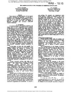
Figure 1: Uniform Linear Array sensing a plane wave propagating across the aperture at an angle φ perpendicular to the array elements. from propagating waveforms. To illustrate this process, we’ll begin by developing a model for a single spatial signal received in the presence of Additive White Gaussian Noise (AWGN) received by our sensor array [3]. In this paper we’ll focus our attention on a Uniform Linear Array (ULA), which is an array that has all of its elements on a line with equal spacing between the elements shown in Fig. 1. We focus our attention on the ULA because of its prevalence and simplicity, but the approach we develop can be generalized to any array geometry. The discrete time observations from the ULA can be written as a vector containing the individual antenna observations: y = [y1 y2 ... yM ]T

(1)

where M is the total number of antennas. Because these antennas are separated in space, the ith array element experiences a delay of τi relative to the first sensor: yi = xe−j2πfc τi + σi

(2)

where x is the baseband signal, fc is the carrier frequency, and σi is the sensor noise. Consider a single propagating signal that impinges on the ULA from an angle, θ, shown in Fig. 1. Because the array elements are equally and deterministically spaced, the spatial signal has a difference in propagation path that results in a time delay of d sin θ (3) c between two adjacent antennas where c is the rate of prorogation through the medium, usually taken to be c = 3 × 108 . Taking the delay of the ith array element with respect to the first element in the array we get τ (θ) =

d sin θ (4) c As you can see from Fig. 1, the delay is a function of the AoA, θ. Each antenna measures a phase difference τi (θ) = (i − 1)

φ(θ) = [1 ei2πfc τ2 (θ) ... ei2πfc τM (θ) ]

(5)

which corresponds to the time delay of the signal at each antenna relative to the first antenna. Because the delay is a function of θ, measuring the array response vector, (5), is equivalent to determining the AoA of the impinging signal.

We can now write the full-array discrete time model as y = φ(θ)x + σ

(6)

The key step for the wideband device is to estimate the AoA, θ, of the other interfering narrowband devices so that it can determine the subspace, w, orthogonal to (5) wH φ(θ) = 0

(7)

and nullify the interference by projecting the received signals onto this subspace. Thus the power of the filtered signal at the spatial location of the interfering devices is negated: 1X H H v = wH yy w = 0 (8) n t In the next section we’ll analyze conventional approaches to angle of arrival estimation, focusing on why Nyquist sampling in the antenna space entails a large plurality of antennas in order to estimate the AoA of interfering signals with high resolution.

3.

CONVENTIONAL SPATIAL DEGREE OF FREEDOM ESTIMATION

We first discuss conventional methods for estimating the DoFs occupied by other secondary devices. The key principle here is Nyquist sampling in the angle domain, and as we discuss below, many of the same constraints apply here. The basic premise behind spatial DoF estimation is to scan through a fine grid in Θ-Space and observe at what angles significant energy is passed through. Implicitly, this scanning is defined under the following model y=

N X

xi φ(θ = i) + σ = Φx + σ

(9)

i=1

where Φ = [φ(θ = 1) φ(θ = 2) ... φ(θ = N )]

(10)

and x = [x1 ... xN ]T with each xi corresponding to the power of the multipath component arriving at θi . {θi }N i=1 represent the sampling points in Θ-Space over a fixed sampling grid of size N . Now let’s consider the scenario where we have T spatial signals arriving at angles {θ1 , ..., θT } with corresponding powers {p1 , ..., pT }. The array measures y, the superposition of these plane waves along with noise. In this scenario, the nonzero components of x should reflect the corresponding values of p while the rest of the entries in x are zero valued. So to summarize, the mapping from the observed signal to Θ-Space is y(n) = Φx + σ 

ei2πfc τ1 (θ1 ) .. . ei2πfc τM (θ1)

 =

i2πfc τ1 (θN ) 



x1 x2 .. .



  ... e     .. ..  + σ (11)  . .   i2πfc τM (θN ) x  ... e N −1 xN

where all of the components of x are zero except in T locations corresponding to {θi }Ti=1 . The main objective is to identify which spatial degrees of freedom are occupied and which ones are available, i.e. estimate the set of angles θ1 . . . θT . In other words, we have

Figure 2: The black lines represent the incoming wavefront of the source signals. Fig. 2A represents the spatial resolution of a larger antenna array while Fig. 2B represents the spatial resolution of a much shorter antenna array (notice that the shorter antenna array is no longer able to distinguish between the two wavefronts at angles θ1 and θ2 ). a sampled signal which varies with the angle of arrival θ, and we are applying sampling to estimate this signal. As expected, the fundamental limits from Nyquist sampling apply here, i.e. number of samples and sampling frequency. For a spatial signal this translates to length of the antenna array (dictates number of samples) and antenna spacing (dictates sampling frequency) [3]. We briefly explain both these constraints intuitively below. First, in order to separate between two plane waves in space (with different angles of arrival), they must differ by at least one period over the length of the antenna array. For the uniform linear array considered in this paper, this amounts to δθ = λ/D

(12)

where λ is the wavelength of the propagating signal and D is the total antenna array length. δθ is related to the sampling grid as N = 180/δθ and is the angle resolution in radians we can achieve with the length D, the larger the antenna array length, the higher resolution we can achieve in our angle estimation. For example in Fig. 2, if the antenna array length is insufficient, the array will be unable to distinguish between two signals arriving from adjacent angles and there will be fewer degrees of freedom to work with. The second factor, analogous to sampling frequency in Nyquist sampling, is antenna spacing. Just like sampling less than the Nyquist sampling rate leads to aliasing, a larger antenna spacing (i.e. a smaller sampling frequency) leads to aliasing in the angle of arrival space. For the linear antenna array considered in this paper, the spatial sampling frequency Us is defined as follows: 1 (13) d The spatial sampling frequency has to be normalized with respect to the wavelength of the signal. As with temporal signals, the phase difference between signals is a direct function of the spatial frequency (U), and because of the uniform spacing of the array, the relationship is given by Us =

U =

sin θ λ

(14)

We then have a notion of normalized spatial frequency defined by u=

d sin θ U = Us λ

(15)

The normalized spatial frequency is unambiguous for 0 ≤ u ≤ 1 and because the full range of angles is 0 ≤ θ ≤ 180, the sensor spacing must be d≤

λ 2

(16)

to prevent spatial ambiguities. Another way to interpret (16) is to consider the fact that the waveform should be sampled at more than two points per wavelength. Otherwise the wave arrival direction becomes ambiguous. If the interarray separation exceeds (16), then spatial aliasing will occur in the reconstruction of the signal. These two physical factors dictate that whitespace systems operating in beachfront spectrum (700 MHz) and intending to use beamforming would require an antenna array length of 24.6 meters and contain 115 array elements in order to achieve 1◦ spatial resolution. Such numbers speak for themselves, the onerous requirements significantly limit our ability to build small, low complexity devices which are able to exploit a wide range of spatial DoFs. This motivates us to find ways to minimize the number of spatial samples without introducing spatial aliasing and maintaining angular resolution. In the next section we discuss how we leverage compressive sensing to solve this problem, i.e., how to use compressive sensing to estimate angles of arrival with high resolution, yet use a small number of antenna.

4.

But how compressible is our signal in the spatial domain? As we discussed, empirical measurements have shown that for indoor environments, T is on the order of 4 or 5 clusters. For instance, if we choose N = 180, giving us an angular resolution of 1◦ over a half circle, our signal has only 5 nonzero components out of 180, more than sparse enough to apply compressive sensing. With this sparse representation of the signal in the spatial domain, we can now use Compressive Sensing as a tool to solve our main objective: identifying which spatial DoFs are occupied and which ones are available. Compressive Sensing (CS) suggests that if a signal x is sparse, the sampling process can be designed so as to acquire only the essential information [7]. This allows for signal acquisition with sampling rates far less than those of traditional sampling methods. Given that we know Φ, the angle to array signal mapping at the Nyquist sampling rate, and the fact that these signals are compressible in Θ-Space, we can accurately reconstruct the signal if we project the N -dimensional vectors onto a random basis that is constituted with random linear combinations of the basis functions in Φ. This allows us to spatially sample the signal at sub-Nyquist rates, meaning that we can use fewer antennas and maintain the same angular resolution. Using spatial compressive sensing, our physical array is composed of K antennas and is characterized as: y = AΦx + σ

where A is a random projection matrix and is of size K ×M , Φ is M × N , and x is an N × 1 vector where the non-zero components represent a source’s signal in the spatial grid at angle θi . The vector of sparse angles, x, is recovered by minimizing the `1 norm of x subject to a constraint:

COMPRESSIVE SPATIAL SAMPLING

Experimental studies done over the past few years have shown that wireless channels tend to exhibit a sparse spatial structure, which tends to become more pronounced as the number of antennas on the receiver is increased. This sparse spatial structure is an artifact of the numerous obstacles and reflectors in the physical environment which cause multipath components to appear in clusters [4][5]. For instance, in [4] they found that for an 8x8 MIMO system in an indoor propagation environment, its transmissions on average arrive at the receiver in 4.4 clusters with a mean cluster azimuth spread of 5.5◦ . This means that 13% of the possible AoA contain significant contributions from clustered multipath components, while the rest of the AoA are essentially free. This observation was exploited in [5] to perform compressed channel estimation using training signals. However, we unfortunately cannot use training symbols because we have assumed no cooperation amongst whitespace devices. Remember that from our problem setup, we have T dominant paths arriving at angles {θ1 , ..., θT }. If we discretize Θ-Space into N distinct angles, T of these will exhibit significant power while the rest will consist of noise. If T 12 antennas while MVAB’s performance slowly improves as the number of antennas increases. In the following simulations, let’s dig down deeper into the reasons why the traditional method, MVAB, requires significantly more antennas than Spatial Compressive Sensing to obtain the same angular resolution.

5.1

Effects of Antenna Array Length

Let’s first look at the effects of the physical constraints we discussed in Section II, antenna array length and interarray spacing, on the MVAB direction estimation method. The beamformer is presented y from (9) and attempts to estimate the resulting spatial power spectrum. As discussed in Sec. II, the array geometry and array element placement play a significant role in the receiver’s ability to resolve spatial information. Our first simulation shown in Fig. 6 shows the effects of antenna array length on resolvable angular resolution. A total antenna array length of 12.9 meters, 60 antennas with λ/2 spacing, are required to obtain 1.9099

Number of Antennas = 15 || Antenna Spacing = 2λ 20 10 0

−80

−60

−40

−20

0

20

40

60

80

60

80

Number of Antennas = 24 || Antenna Spacing = λ 20 10 0

−80

−60

−40

−20

0

20

40

Number of Antennas = 60 || Antenna Spacing = λ/2 20 10 0

−80

−60

−40

−20

0

20

40

60

80

Direction of Arrival Angle (degrees)

Figure 5: Simulation 2: As we increase the spacing, decreasing the number of antennas, the spatial sampling begins to introduce aliasing.

angular resolution for us to distinguish signals 2 and 3. If we try to reduce the number of spatial samples by reducing the number of antennas, we subsequently reduce the antenna array length and are unable to obtain sufficient angular resolution to resolve signals with sufficient precision.

5.2

Effects of Inter-Array Spacing

Next let’s look at the effects of inter-array spacing for discrete spatial sampling. Fig. 5 shows the results of simulation 2 which has the same source parameters as simulation 1. Here we maintain an antenna array length of 12.9 meters, which is what we demonstrated was necessary for 1.9099◦ angular resolution, while reducing the number of spatial samples taken by increasing the spacing between the array elements. As you can see when the inter-array spacing is greater than λ/2, aliasing occurs and the sampled spatial spectrum does not equal the true spatial spectrum. As we discussed, the waveform has to be sampled at more than two points per wavelength, otherwise the wave arrival direction becomes ambiguous. The spatial aliasing effect is seen in Fig. 4 (a)-(c). From these results, we see that if we try to reduce the number of spatial samples by increasing the inter-array distance to maintain antenna array length, spatial aliasing will distort the signal’s spatial information.

5.3

Spatial Compressive Sensing

Here we analyze the performance of our Spatial Compres-

Signal Power Signal Power

True Signal 25

25

Compressive Sensing Signal vs. MVAB for 40−Sparse Signal 25

15

20

Signal Power

10 5 0

−80

−60

−40

−20

0

20

40

60

80

Compressive Sensing Signal || Number of Antennas = 12 20

10

5 10 5 0

0 −80

−60

−40

−20

0

20

40

60

80

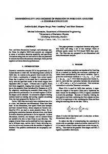
Figure 6: Simulation 3: Spatial Compressive Sensing allows us to achieve an angular resolution of 2 degrees with only 12 antennas, as opposed to 60 with traditional methods. sive Sensing approach and demonstrate that using significantly fewer spatial samples, we can maintain angular resolution and avoid spatial aliasing. First we construct an array response vector Φ such that the ith column corresponds to a potential source at angular location θi . We set the number of columns, N = 180, which gives us an angular resolution of 1◦ over a half-circle. We then project the desired signal x onto a random basis constituted by random linear combinations of the array response vector. This allows us to use significantly fewer antennas, only 12 compared to the 60 needed for MVAB, to perfectly preserve the spatial content of the signal. These results are pretty convincing and validate our initial hypothesis from a theoretical standpoint Sub-Nyquist spatial sampling can be achieved with spatial compressive sensing.

−80

−60

−40

−20

0

20

40

60

80

Direction of Arrival Angle (degrees)

Figure 7: Simulation 4: The signal sparsity is such that Spatial Compressive Sensing is slightly past the limits of effective operation with a normalized error of .02091 whereas the MVAB is more accurate and has a normalized error of 3.92 × 10−6 on practical cognitive device design. The first is that sufficient angular resolution can be obtained using a reasonable number of antennas. Whereas it takes on the order of 75 antennas using traditional AoA estimation techniques, we’ve demonstrated that the same resolution can be achieved using fewer than 12 antennas with Spatial Compressive Sensing. Second, fewer spatial samples means that there will be less latency in the channel estimation, allowing for more agile devices. Spatial compressive sensing is a first and important step in building low power spatially adaptive whitespace devices. In the near future we expect to implement this technique on software radios, and generalize it to simultaneously detect available degrees of freedom in both space and frequency dimensions.

Limits of Spatial Compressive Sensing

Lastly we discuss the limitations of Spatial Compressive Sensing. According to (21), for our Spatial Compressive Sensing approach to use fewer spatial samples than MVAB while achieving an angular resolution of 1.5◦ the signal can have at most 38 nonzero components out of 120. To achieve this angular resolution, MVAB needs at least 75 antennas - an unrealistic number for practical systems. The point where MVAB becomes more effective than Spatial Compressive Sensing is when they require a similar number of antennas. Shown in Fig. 7, we simulate the scenario where there are 40 nonzero components out of 120. Observe that the performance of Spatial Compressive Sensing with 70 antennas slightly underperforms that of MVAB, slightly misdetecting a few sources at low powers at certain angles. We cannot use fewer than 70 antennas or else the performance would be even worse (70 antennas is an impractically large number but we are stress testing the system, so we need to examine the boundary cases). As you can see, the limitation of spatial compressive sensing is that the signal must be sufficiently sparse in the spatial domain.

6.

15

15

Direction of Arrival (degrees)

5.4

True DoA MVAB − 75 Antennas Spatial CS − 70 Antennas

20

CONCLUSION

In this paper, we have described a Spatial Compressive Sensing approach for estimating the spatial DoFs in a whitespace environment possibly occupied by several cognitive devices. We’ve demonstrated that using Spatial Compressive Sensing allows a system to achieve high angular resolution with the acquisition of significantly fewer spatial samples. Spatial Compressive Sensing has numerous implications

7.

REFERENCES

[1] S. Haykin, “Cognitive Radio: Brain-Empowered Wireless Communications,” IEEE Journal on Selected Areas in Communications, vol. 23, no. 2, 2005. [2] R. Zhang and Y.-C. Liang, “Exploiting multi-antennas for opportunistic spectrum sharing in cognitive radio networks,” IEEE J. Sel. Topics Sig. Proces., vol. 2, no. 1, Feb. 2008. [3] D. Manolakis, V. Ingle, S. Kogon, “Statistical and Adaptive Signal Processing, Boston: McGraw-Hill, 2000. [4] N. Czink, X. Yin, H. Ozcelik, M. Herdin, E. Bonek, B. Fleury, “Cluster Characteristics in a MIMO indoor propogation environment,” IEEE Trans. Wireless Communications, vol. 6, no. 4, pp. 1465-1475, Apr. 2007. [5] W. Bajwa, J. Haupt, A. Sayeed, R. Nowak, “Compressed Channel Sensing: A New Approach to Estimating Sparse Multipath Channels”, Proceedings of the IEEE, July 2010 [6] D. Wipf, S. Nagarajan, “Beamforming using the RVM”, Proceedings of the International Conference on Machine Learning, 2007. [7] E. Cand´es, J. Romberg, and T. Tao, “Stable signal recovery from incomplete and inaccurate measurements,” Communications on Pure and Applied Mathematics, vol. 59, no. 8, pp. 1207-1223, 2006.