their own, but rather judiciously lease bandwidth from a collocated cellular network (CN). We develop a distributed mechanism that such WMNs can use to ...
Cognitive WMNs: A Distributed Mechanism for Leasing Cellular Network Bandwidth S. Toumpis∗ , I. Tselekounis∗ , G. D. Stamoulis∗ , H. Meyer† , A. Hess† , K. A. Hummel† ∗ †
Informatics Department, Athens University of Economics and Business (AUEB), Greece
Entertainment Computing Group (formerly Distributed Systems Group), Univ. of Vienna, Austria Abstract We study flow optimization in cognitive Wireless Mesh Networks (WMN) that do not possess any bandwidth of their own, but rather judiciously lease bandwidth from a collocated cellular network (CN). We develop a distributed mechanism that such WMNs can use to optimize their traffic given their own traffic needs and the cost that the CN is charging for the use of its bandwidth. We evaluate the mechanism in a synthetic scenario using the topology of an actual deployed WMN and time-varying traffic requirements induced from actual vehicle mobility traces. Simulations show that the mechanism can track well the changes in the traffic requirements of the WMN, continuously keeping close to the optimum operation point.
I. I NTRODUCTION Wireless Mesh Networks (WMN) have recently become a very popular type of infrastructure, serving a multitude of applications such the offering of alternative IP interconnection, the support of vehicular networks, etc. However, in WMNs, a number of factors contribute to an often severe bandwidth shortage: 1) Communication is often over the ISM band, which has limited bandwidth and is susceptible to unpredictable and unresponsive levels of interference. 2) Communication is multihop, so that each packet must typically be transmitted multiple times over the wireless medium. 3) Wireless mesh routers with access to the Internet, or routers near them, must relay large volumes of traffic and as a result bottlenecks are formed. 4) The volume of the data files that must be transported is often significant. One way of alleviating the bandwidth shortage is to adopt a cognitive network approach [1] under which the WMN uses bandwidth that is available to nearby cellular networks (CNs), whenever it happens to be underutilized by them. Indeed, the fluctuating pattern of cellular type traffic, where voice predominates, implies that, at least for parts of the day and most of the night, large portions of the bandwidth remain unused [2]. In this work, we develop and evaluate a framework under which this potential synergy between WMNs and CNs can materialize. In Section II we develop a system model that consists of a WMN and a set of CN channels that
are available for use, at a price. The WMN consists of nodes and links. The topology and the technology used are such, that for each CN channel there is a subset of links that will interfere with the operation of that channel, if traffic passes through them. Furthermore, each link may interfere with more than one channel. Each WMN node derives a utility value by inserting flow in the network if it is a source, or removing flow from the network, if it is a sink, given by a concave utility function. Each WMN node derives a concave utility by inserting flow in the network, if it is a source, or removing flow from the network, if it is a sink. Each channel is available for use but for a price which is a convex function of the aggregate level of interference caused to it by all interfering links of the WMN. Finally, the use of each link is also subject to some convex cost. We show that the point of socially optimal operation, that maximizes the sum of the utilities of all nodes, minus the costs of all channels and links, can be found by solving a monotropic program, which is a special type of convex optimization problem. In Section III we show that this problem can be solved through a distributed mechanism executed by agents located throughput the network. Each agent only needs to communicate with agents that are physically close. The mechanism is justified in terms of a partial Lagrangian dualization of the convex optimization problem. The mechanism provably establishes the point of optimal operation when the input to the problem does not change. Furthermore, when the input changes, for example due to mesh client mobility and/or the fluctuating availability of the cellular bandwidth, a properly modified version of the mechanism aims at producing traffic flows close to the optimal one. In Section IV we evaluate the mechanism in a synthetic scenario using the topology of the Funkfeuer WMN [3] currently deployed in Vienna and where the traffic that the WMN must support originates from vehicular mesh clients whose mobility is based on actual vehicular mobility traces collected from the same city. We show that the distributed mechanism succeeds in keeping the network close to its optimum operation point, despite the fact that this operation point is constantly changing due to the mobility of clients. In Section V we present an overview of related work in the field of cognitive WMNs. In Section VI we discuss some limitations of our work, outline future work, and conclude. II. S YSTEM M ODEL We model the WMN in terms of a set N of N nodes, indexed by n = 1, 2, . . . , N and a set L of L directed links, indexed by l, where l = 1, 2, . . . , L. Let s(l) ∈ N be the node from which the link starts, i.e., the transmitter, and e(l) ∈ N be the node where the link ends, i.e., the receiver. We permit the possibility that there are multiple links starting and ending at the same pair of nodes (we explain why later on). The flow of data packets along link l, measured in bps, is denoted by xl . Let x = (xl : l ∈ L) be the flow vector. The flow xl must be non-negative and not exceed a maximum value, i.e., 0 ≤ xl ≤ xmax . The maximum l value xmax can be thought of as a capacity constraint for that link and depends on the transceiver technology used, l
and perhaps also arbitrary constraints set by the modeler. Let xmax = (xmax : l ∈ L). Based on the above, l 0L ≤ x ≤ xmax ,
componentwise, where 0L is a L-sized vector with zero components. We assume, for each link l, a convex link cost function hl (xl ), which models the cost of having flow xl through link l. The link cost function can model a variety of costs, for example energy costs. Let X
sn =
xl −
l∈L:n=s(l)
X
xl
l∈L:n=e(l)
be the divergence of the flow vector at node n. The divergence expresses the rate, in bps, with which the node inserts data in the network (if positive) or removes data from the network (if negative) so that information is conserved, given the flows of traffic along ingress and egress links. Let s = (sn : n ∈ N ) be the divergence vector. We assume that the divergence is subject to optimization, but must stay within an upper and a lower bound, ≤ sn ≤ smax i.e., smin n . These bounds may be used to express restrictions on the technology. For example, if node n n cannot process outgoing traffic with a rate greater than M > 0, then we can set smax = M . The bounds can n
also be used to restrict the behavior of the nodes. For example, if a node n must act strictly as a sink, we can set smax = 0; if n is a source producing data with a fixed, inelastic data rate s > 0, we can set smax = smin = s. Let n n n smax = (smax : n ∈ N ), smin = (smin : n ∈ N ). Based on the above, n n smin ≤ s ≤ smax .
For each node n, there is a concave utility function Un (sn ) that expresses the utility the node derives by having its divergence equal to sn . Various choices are possible for the utility function, each modeling a different kind of node. For example, if we set Un (sn ) =
sn ,
sn ≥ 0,
−∞,
sn < 0,
then node n is a source that inserts traffic into the network, and its satisfaction increases linearly with the volume of that traffic. If, on the other hand, Un (sn ) =
log(1 + sn ),
sn ≥ 0,
−∞,
sn < 0,
then the node is a source whose satisfaction increases logarithmically. As a last example, if, −∞, sn > 0, Un (sn ) = −sn , sn ≤ 0,
then node n is a sink, that is not allowed to insert traffic, and its satisfaction increases linearly with the amount of traffic it receives. In contrast to the common WMN scenario where channels are frequency ranges either used by a single link or possibly shared by many links, in our setting we define a channel to be the whole bandwidth used by a specific cell of a nearby CN. Therefore, there is one channel for each cell, and so in the following the words channel and cell will often be used interchangeably. Note that there may be more than one CN in the area, so that two channels may belong to different CNs. As frequencies are reused in CNs, there will be subsets of distinct channels sharing the same frequency range. Let C be the set of channels, indexed by c = 1, 2, . . . , C . Let rc be the reservation level of channel c, and r = (rc : c ∈ C) be the reservation vector. Reservation levels are unitless, and express how much the respective channel is used as a function of the traffic at all links. Each reservation level rc must be nonnegative and less than a maximum value rcmax . A reservation level equal to the maximum rcmax corresponds to the maximum amount of channel c usage permitted by the CN. Let rmax = (rcmax : c ∈ C), so that 0C ≤ r ≤ rmax ,
where 0C is a C -sized vector with zero components. As discussed in the introduction, channels are not available for free, but come at a cost that is a function of their reservation level rc . Therefore, for each of the C channels, we define a convex channel cost function fc (rc ). In principle, the channel cost function combines two terms: the cost incurred to the cellular network by not having the channel available, which must be offset by the WMN, and also a term corresponding to the profit the cellular network expects by renting off its channel. Due to the spatially distributed nature of the wireless channel, when a node transmits over a link, we expect that the operation of possibly more than one channel will be interfered with, and each of these must be reserved. In addition, we expect that each channel can possibly be interfered with by more than one link. This arbitrary coupling between links and channels is modeled as follows: let Rcl , the reservation coefficient for channel c and link l. We require Rcl ≥ 0. Let the reservation matrix R = {Rcl } of size C × L. We require the reservation vector and the link flows to be connected through the following basic relation: r = Rx ⇔ rc =
L X
Rcl xl ,
∀c ∈ C.
l=1
Therefore, the reservation coefficients model the coupling between the channels and the links. The precise value of the coefficients will depend on the topology, the transceiver technology used, the specific frequency ranges used by the CN channels, and other aspects of the hardware used. For example, if a channel c and a link l are in physically disparate locations, we anticipate that using the link will not affect the operation of the channel, therefore Rcl = 0. If the link and the channel are physically near, but the link uses strongly directional antennas and the scattering of its transmitted signal stays below some minimum level, then still Rcl = 0. If, however
activating the link causes interference with the normal operation of the channel, Rcl > 0, and the larger Rcl is, the more of channel c is required in order to support a given volume of traffic across link l. Establishing the precise value for the coefficients goes beyond the scope of this work, however we stress that our model is very general and can capture a large variety of hardware setups. Remember that we have allowed the possibility of multiple links connecting the same transmitter/receiver pair. Therefore, we can model the scenario in which a transmitter-receiver pair can choose one of many sets of channels with which it will interfere, each set corresponding to a different link l and a different column of the coefficient matrix R. For example, let us assume the bandwidth is borrowed from a CN with a reuse factor M . Therefore, there are M frequency ranges, each one used by multiple cells. As already discussed, in this setting each channel is associated with a cell. We could have M links connecting a pair of nodes, each link using a different frequency range, and so interfering with those nearby channels using the same frequency range. We now have all the components of the flow optimization problem: Problem I: Utilities Minus Costs (U-C) Maximization maximize: subject to:
n=1 Un (sn )
PN
sn =
P
−
c=1 fc (rc )
PC
xl −
l=1 hl (xl ),
(1)
∀n ∈ N ,
(2)
PL
xl ,
l∈L:n=e(l)
l∈L:n=s(l)
rc =
P
−
PL
l=1 Rcl xl ,
, 0 ≤ xl ≤ xmax l smin ≤ sn ≤ smax n n , 0 ≤ rc ≤ rcmax ,
∀c ∈ C,
(3)
l ∈ L,
(4)
n ∈ N, c ∈ C.
(5) (6)
Formally, the optimization variables are x, s, and r. However, due to the existence of the equality constraints, one may adopt the view that the flows x are the only ones subject to optimization, and they affect the objective function through the "auxiliary" variables s, r. This is the problem the WMN must solve in order to maximize the profit the WMN makes out of transporting traffic minus the cost it pays to lease the channels used to transport the traffic and the cost of using the links (expression (1)), subject to the constraints that information is conserved (constraints (2)), the proper amounts of reservations are made for each channel (constraints (3)), and that flows, divergences, and reservation levels are between accepted bounds (constraints (4), (5), and (6) respectively.) Note that the optimization problem is convex, as the utilities have been assumed concave, the channel and link costs convex, and all constraints are linear. Furthermore, the optimization function is separable, therefore this is a monotropic program, for which very efficient centralized solution methods exist [4]. Next, in Section III we show how to solve it using an approach based on duality that can be implemented in a distributed manner.
N
Node set
N n
xl
Flow at link l
Node set
x
Node index
xmax l max
rc
reservation level of channel c
Flow vector
r
Reservation vector
Maximum flow at link l
rcmax
Maximum reservation level
max
L
Link set
L
Number of links
0L
L-sized vector of zero components
0C
C-sized vector of zero components
l
Link index
sn
Divergence at node n
Rcl
Reservation coef. for channel c and link l
C
Channel set
s
Divergence vector
R
Reservation matrix
Number of channels
smin n
Lower bound of s
Un (sn )
Utility function at node n
Channel index
smax n
C c s(l) e(l)
start of link l end of link l
x
Upper bound of x
r
Upper bound of r
Maximum divergence at node n
fc (rc )
Channel cost function at channel c
min
Lower bound of s
hl (xl )
Channel cost function at link l
max
Upper bound of s
s s
TABLE I N OTATION INTRODUCED IN S ECTION II
Also note that we cast our problem as a single commodity optimization problem. Therefore, each packet inserted in the network does not have a specific destination, but may be received by any node whose divergence can be negative. This assumption makes sense for WMNs, where typically nodes are interested in communicating with any mesh router connected to the Internet, and the choice of mesh router is not important. However, the multicommodity case can also be formulated in a similar manner. This is the subject of future work. In Table I we have collected all the notation introduced in this section. III. D ISTRIBUTED F LOW O PTIMIZATION USING D UALITY A. The dual problem As discussed, Problem I is straightforward to solve, as it is convex, and furthermore, a monotropic program. However, among the variety of solution methods existing, we would like to use a method with the following features: 1) It can be implemented through a distributed mechanism using agents placed throughout the network, and 2) the used mechanism can track the optimal point of operation as the problem changes, due to changes, for example in the utility and cost functions. In this section we introduce one such mechanism, based on Lagrangian duality. We start by formulating a dual problem. To simplify the exposition, we will make the additional assumption that the utility function is strictly concave, and that both the link and channel cost functions are strictly convex. This ensures that the optimum values of x, s, r, denoted by x∗ , s∗ , r∗ respectively, that solve Problem 1, are unique. Note that any convex function can be
made strictly convex by the addition of a strictly convex term that can be arbitrarily small. The extension to the
non-strictly convex case is straightforward, but is postponed for future work. First, let us hypothetically assume that nodes are allowed to violate the data conservation constraint (2) provided they sell any excess traffic that gets accumulated at them at a node price λn ∈ R, for node n, or buy any traffic they lack at that same price. This transaction is done with an external, hypothetical market. The resulting profit (or loss) is added to the objective. Let λ = (λn : n ∈ N ) be the node price vector. Secondly, let us assume that the network is allowed to violate constraint (3), and so reserve more or less channel bandwidth than the bandwidth needed. However, any excess, unused bandwidth must be sold off to the external market for a channel price µc ∈ R, for channel c, and any missing bandwidth must be bought at the same price. The resulting profit (or loss) is also added to the objective. Let µ = (µc : c ∈ C) be the channel price vector. We note that both node prices and channel prices can be negative, in which case the above interpretations in terms of financial transactions must be interpreted accordingly. With these modifications to the original problem, the new, relaxed objective function becomes the Lagrangian L(x, s, r; λ, µ) ,
N X
Un (sn ) −
n=1
+
X
λn sn −
X
xl +
l:s(l)=n
λe(l) − λs(l) −
+
hl (xl )
l=1
"
l=1 N X
L X
n=1
=
fc (rc ) −
c=1
N X
L X
C X
C X
xl +
l:e(l)=n
C X
" µc rc −
c=1
!
L X
# Rcl xl
(7)
l=1
# xl − hl (xl )
(8)
[µc rc − fc (rc )] .
(9)
Rcl µc
c=1
[Un (sn ) + λn sn ] +
n=1
C X c=1
The second equality comes from rearranging terms. Using these modifications, the new optimization problem becomes Problem 2: Relaxed U-C Problem maximize: subject to:
L(x, s, r; λ, µ) 0 ≤ xl ≤ xmax , l smin ≤ sn ≤ smax n n , 0 ≤ rc ≤ rcmax ,
l ∈ L, n ∈ N, c ∈ C.
Observe that the constraints on the upper and lower bounds of the flows, divergences, and reservation levels remain. Also observe, from expression (9), that the Lagrangian can be written as the sum of L terms each involving a single flow, N terms each involving a single divergence, and C terms each involving a single reservation level. Therefore, Problem 2 breaks into the following L + N + C problems, that can be solved in parallel, each involving a single optimization variable, a one-dimensional objective function, and a single constraint:
Problem 3a: Links (l = 1, . . . , L) �
maximize:
λe(l) − λs(l) −
PC
c=1 Rcl µc
�
xl − hl (xl )
0 ≤ xl ≤ xmax . l
subject to:
Problem 3b: Nodes (n = 1, . . . , N ) maximize:
Un (sn ) + λn sn ,
subject to: smin ≤ sn ≤ smax n n . Problem 3c: Channels (c = 1, . . . , C ) µc rc − fc (rc ),
maximize:
subject to: 0 ≤ rc ≤ rcmax . Observe that, due to the strict convexity of the costs and the strict concavity of the utility functions, each of these problems has a unique solution. Also observe that in all cases we wish to maximize a linear function minus a convex function over a compact set. The resulting maximum, when viewed as a function of the coefficient of the linear term, is known in the literature as the conjugate function of the convex function [5]. Let the dual function q(λ, µ) be the maximum objective of Problem 2, i.e., q(λ, µ) = argmax L(x, s, r; λ, µ), x,s,r
which can be established by solving Problems 3a, 3b, 3c. Consider also the following, dual problem: Problem 4: Dual Problem minimize:
q(λ, µ).
In this problem, the optimization is over λ and µ and there are no constraints. Conceptually, the above problem is equivalent to the external market trying to find such prices, so that the net profit of the WMN is minimized. Using this interpretation, we expect that, once prices are selected in this manner, the WMN refrains from using the external market. Indeed, if the market has selected a node price such that it is buying data from the network at that node, then we expect that if this price increases incrementally, then the profit of the network would also increase by an incremental amount of the same order. Indeed, by standard duality theory [6], the optimum value of Problem 4 (which is a minimization) coincides with the optimum value of Problem 1 (which is a maximization); furthermore, the optimum values x∗ , s∗ , r∗ can be found also by solving Problem 2, using for λ and µ the optimum values, λ∗ and µ∗ , of Problem 4. Therefore, we can solve Problem 1 by solving Problem 4, and then using its solution, λ∗ and µ∗ , to solve the (much simpler) Problem 2. Next, we show an algorithm for solving the dual problem.
B. A centralized algorithm for solving the dual problem In order to solve Problem 4 (and subsequently Problem 1), we note that, by standard duality theory and the strict convexity of the problem (Prop. 6.1.1, [6]), the dual function is continuously differentiable, and for each pair of price vectors λ, µ, the gradient ∇q(λ, µ) of the objective function q(λ, µ) can be found using the constraint violations of Problem 1. In particular, at the prices λ, µ, the value of the component ∇qλn of the gradient corresponding to the price λn is X
∇qλn (λ, µ) = sn −
xl +
l∈L:n=s(l)
X
xl ,
∀n ∈ N
(10)
l∈L:n=e(l)
and the value of the component ∇qµc of the gradient corresponding to the price µc is ∇qµc (λ, µ) = rc −
L X
Rcl xl ,
∀c ∈ C,
(11)
l=1
where the vectors x, s, r are the solutions of Problems 3a, 3b, 3c, for the above choices of prices λ, µ. These equations can be motivated intuitively. Indeed, the right hand side of (10) equals the amount of traffic exported by node n to the external market, and we expect this to be equal to the rate with which the profit increases with an increase in the price λn , which in turn should be equal to the component of the gradient corresponding to the price λn . Equation (11) has a similar interpretation. As a formula for the gradient is available, the following centralized gradient descent algorithm can be used: Centralized U-C Algorithm INPUT:
smin ,
smax ,
xmax ,
rmax ,
hl (·), Un (·), fc (·), R.
STEP 1 (INITIALIZATION) Initialize prices λn , µc to arbitrary values λ0n , µ0c , for all n = 1, . . . , N, c = 1, . . . , C . Let the iteration level i = 0. STEP 2 Set i = i + 1. Solve Problems 3a, 3b, 3c. STEP 3 Find all prices λin , µic in the i-th iteration using i−1 1) their values in the previous iteration λi−1 n , µc , and
2) the flows xil , divergences sin , and reservation levels rci found in STEP 2, through which the gradient components ∇qλi n , ∇qµi c can be found, using equations (10), (11).
Use the formulas: λin = λni−1 − a∇qλi n ,
(12)
µic = µi−1 − a∇qµi c , c
(13)
where a is a fixed, universally known, step size. STEP 4 IF Termination Condition is not satisfied GO TO STEP 2.
Regarding the termination condition, a variety of choices is possible. For example, we can stop the execution if the improvement in the dual function over a given number of iterations is smaller than a given threshold. This algorithm is guaranteed to terminate, under weak assumptions on the decreasing step size [6]. Indeed, it can be shown theoretically that both the distances of the primal and dual objectives from their optimum values and the distances of the primal and dual optimization variables from their optimum values all tend to zero as the number of iterations goes to infinity, and assuming that the INPUT of the problem does remains fixed. Once the algorithm terminates, the optimal solution of Problem 1 can be established by solving Problems 3a, 3b, 3c, for the optimal prices λ∗ , µ∗ found. C. Distributed solution of time-invariant problem With minor modifications in its essential operations, the algorithm of Section III-B can be executed in a distributed manner, by use of a number of agents placed across the network. In particular, there will be needed: 1) a link agent l (LAl) for each link l, responsible for the iterative solution of the l-th Problem 3a. 2) a node agent n (NAn) for each node n, responsible for the iterative solution of the n-th Problem 3b. 3) a channel agent c (CAc) for each channel c, responsible for the iterative solution of the c-th Problem 3c. These agents agree on a periodic schedule under which all steps of the algorithm are executed simultaneously and in a distributed manner across the network as follows: Distributed U-C Algorithm INPUT: Initially, each agent naturally possesses some part of the input. In particular: , and the reservation coefficients Rcl for all channels c it 1) LAl knows hl (·), the step size a, the bound xmax l interferes with (in other words, the l-th column of R). max 2) NAn knows function Un (·), the step size a, and the bounds smin n , sn .
3) CAc knows fc (·), the step size a, and the bound rcmax . STEP 1 (INITIALIZATION) Let the iteration level i = 0. NAn selects an arbitrary initial price λ0n and relays it to the agents of its incident links. Also, CAc selects an arbitrary initial prince µ0c and relays it to the links it is being interfered from. STEP 2 Set i = i + 1. 1) LAl solves the l-th Problem 3a and sends the flow found to the node agents s(l) and e(l) and the channel agents of all channels it interferes with. 2) NAn solves the n-th Problem 3b. 3) CAc solves the c-th Problem 3c. STEP 3 1) NAn finds a new value for the price λin , using (12), and relays it to the agents of its incident links.
2) CAc find a new price µic , using (12), and relays it to the links it is being interfered from. STEP 4 If i < I , where I is a globally known maximum, then GOTO STEP 2, ELSE STOP. Observe that communication is constrained between agents that are physically near. As an example, note that a link agent, in order to solve Problem 3c, needs the node prices of its two adjacent nodes as well as the channel prices of all channels it is using. D. Distributed solution of time-varying problem The algorithm of Section III-C assumes that the input to the problem (i.e., the utility and cost functions and the various bounds) remains fixed. However, it can easily be adapted to changing conditions. The way to do this is to make sure that, during STEP 2, the most updated versions of Problems 3a, 3b, 3c are solved. For example, if the utility function of a node changes, only the agent of that node will have to adjust its problem formulation, and start solving a different problem. The rest of the agents will eventually witness the effects of this change, and adjust accordingly to the new point of operation, through communication with their own neighbors. Formally, let us assume that the variables appearing at the INPUT are changing with time, and so with the iteration i. With respect to the Distributed U-C Algorithm, the following changes are necessary: 1) At each STEP 2, the latest version of the input is used. 2) We remove the termination condition, so that the algorithm is executed ad infimum. 3) At the end of STEP 2, the agents use the prices currently available to them to construct a feasible solution. We refer to the resulting algorithm as the Variable Input Distributed U-C Algorithm. The last modification, i.e., the construction of a feasible solution at the end of STEP 2, is necessary because solving the Problems 3a, 3b, and 3c with any prices other than the optimal ones will in general provide us with a set of vectors x, s, r that are not feasible. Under challenging scenarios, we expect that the algorithm will never converge to the optimum values, and therefore the vectors it will be providing, while possibly close the optimum, will be infeasible. In principle, there can be various solutions to this problem. Here, we discuss only one possibility. To simplify the exposition, we make the further assumption that node 1 is a source for which we have smax = +∞, smin = 0, n 1 whereas for the rest (the sinks) we have smax = 0, smin = −∞. The feasible solution can be constructed, at the n n end of STEP 2, as follows: 1) Channel agents calculate a tentative reservation level rc0 using the formula rc0
where
x0l
=
are the flows calculated during STEP 2.
that rc0 > rcmax .
L X
Rcl x0l ,
l=1 0 rc is guaranteed
to be non-negative, however it is possible
λn
Node price for node n
µc
Channel price for channel c
λ
Node price vector
µ
Channel price vector
L(x, s, r; λ, µ)
Lagrangian
q(λ, µ)
Dual function
∇qλn ∇qµn
gradient of q(λ, µ) corresponding to λn
x
Optimal x
∗
gradient of q(λ, µ) corresponding to µc
∗
∗
r
∗
Optimal s
∗
s
Optimal r
λ
Optimal λ
λin
λ in iteration i
µ
Optimal µ
a
Step size
µic
µc in iteration i
i
Iteration number
TABLE II N OTATION INTRODUCED IN S ECTION III
2) Link agents calculate new flows as follows: x00l = x0l min{1, min{
rcmax }}, rc0
where the second minimum is over all channels the link is interfering with. In other words, when a link discovers that it is violating the reservation constraint of a channel by some factor, it reduces its flow by the same factor. 3) Each CAc calculates a new tentative reservation level rc00 using the formula rc00 =
L X
Rcl x00l ,
l=1
This new reservation level is guaranteed not to violate the maximum reservation constraint. 4) Each node calculates a tentative divergence as follows: sn =
X l∈L:n=s(l)
5) For each n > 1, if
s00n
X
xl −
xl
l∈L:n=e(l)
> 0, then this tentative divergence violates its upper bound constraint. The agent inserts
padding traffic in the network, with rate s00n . If s00n ≤ 0, then that divergence does not violate the constraint, and the node removes traffic from the network with that rate. Note that some of that traffic so removed may be padding. 6) As the divergences of all sinks have been obtained, and the sum of all divergences (including the divergence of the source) must be zero, the source divergence has also been obtained at this point, and is guaranteed to be non-negative. IV. S IMULATIONS We offer a preliminary evaluation of the distributed mechanism in a synthetic scenario based on the Funkfeuer WMN deployed in Vienna, real-life mobility traces of taxis collected at the same city, and simulated input regarding the CN channels and the WMN connectivity, among others. The simulation setup does not comply to reality fully,
18 16 14
y (km)
12 10 8 6 4 2 0
0
2
Fig. 1.
4
6
8
10
x (km)
12
14
16
18
The WMN example of Section IV.
and so should not be seen as a quantitative evaluation of the potential real-life synergy between a WMN and a CN, but as a proof of concept. Our WMN contains 265 nodes placed in the actual locations of Funkfeuer [3] routers in the Vienna. There are 592 links, chosen so that the resulting connectivity closely resembles that of actual WMNs, with a combination
of short range and long range links. The region containing the routers is covered with 100 CN cells arranged in a square grid. Frequency reuse with a reuse factor of 4 is assumed. The WMN supports the download of information by a number of vehicular users, as we describe shortly. We specify the reservation matrix as follows: 1) If link l connects two nodes s, e that exist on the same cell c, then we set Rcl = 1. 2) Let link l connect a transmitter node s and a receiver node e lying on adjacent cells that share an edge. Let c1 be the cell where the transmitter is located, and let c2 the cell that shares the same frequency set with c1
and is closest to the receiver node e. We set Rc1 l = Rc2 l = 1. 3) Let link l connect a transmitter node s and a receiver node e lying on adjacent cells sharing only a common vertex. Let c1 be the cell where the transmitter is located, and let c2 , c3 , c4 the three cells that share the same frequency set with c1 and are closest to the receiver e. We set Rc1 l = Rc2 l = Rc3 l = Rc4 l = 1. 4) All other entries of the reservation matrix are set to zero. To clarify this rule, as a simple example, in Fig. 2 we have plotted a simple, hypothetical cellular network (unrelated to the network used in the rest of the plots) where M = 4, m = 2. There are 4 distinct sets of frequencies, and we have shadowed all cells using each one of them with the same shadowing. We have also placed
1
2
3
4
5
6
7
8
9
10
11
12
15
16
17
18
21
22
23
24
27
28
29
30
33
34
35
36
1
2
13
14
19
20
3
4 5
Fig. 2.
25
26
31
32
6
7
A hypothetical example WMN embedded on a cellular network of frequency reuse factor of 2 × 2. Node indices are italicized and
underlined. Channel/cell indices appear in down right corner of each cell. D
r
A
Length of square region
2
M
Number of cells in each direction
M
m
Reuse factor along x and y axes
u(·)
max
S
Maximum reservation level for all c Maximum received data volume per node
max
x
k(n)
Communication radius Total number of cells, here equal to C Utility of a single vehicular user Maximum traffic flow for all l Number of users per node n
TABLE III N OTATION INTRODUCED IN SECTION IV
N = 7 nodes, and set A equal to a cell diameter, resulting in L = 18 links. The links, along with the channels
they use for their communication, appear in Table IV. The entries of that table can be explained based on the rules above. As a second example, in Fig.3 we have plotted the same cellular setting, with only two links, the link from node 1 to node 2 and the link from node 4 to node 3. Observe that both links will reserve, among their other channels,
channel 21, and therefore these two links cannot coexist in time. Depending on the topology and the transceiver technology, these rules may either be reasonable, or just make sense to a certain extent. However, we believe that the use of the reservation matrix offers enough flexibility so that a variety of environments and transceiver technologies can be modeled in a satisfactory manner.
1
3
2
7
9
8
4
5
6
10
4 11
12
3 13
14
15
16
17
18
19
20
21
22
23
24
25
26
27
28
29
30
31
32
33
34
35
36
2
1
Fig. 3.
A second, hypothetical example in the same cellular setting. (1,2)
14, 16
(2,1)
15, 13
(2,3)
15, 17
(3,2)
16, 14
(3,4)
16, 14, 26, 28
(4,3)
21, 9, 11, 23
(1,4)
14, 16, 26, 28
(4,1)
21, 7, 9, 19
(2,4)
15, 27
(4,2)
21, 9
(4,5)
21, 33
(5,4)
27, 15
(5,6)
27
(6,5)
33, 21
(5,7)
27
(6,5)
33, 21
(6,7)
33
(7,6)
33
TABLE IV T HE CHANNELS RESERVED FOR EACH OF THE LINKS (i, j) OF THE WMN OF F IG . 2
Regarding the channel costs, we set fc (rc ) = rc2 , and also 0 ≤ rc ≤ rmax = 50. Therefore, the prices of the CN bandwidth becomes steeper as the WMN reserves more of it, and the CN is forced to operate closer to its capacity. Regarding the link costs, we set hl (xl ) = x2l , and also 0 ≤ xl ≤ xmax = 5. Our motivation for using this link cost is that it promotes load balancing, as links with large traffic volumes are heavily penalized. We are simulating a downloading scenario as follows: Among the nodes, one, centrally located, is chosen as a gateway. Let this be node 1. We set smin = 0, smax = 26500, so that the gateway can only insert traffic. All other 1 1
nodes are required to remove traffic, and in particular we set smin = −100 and smax = 0 for all n 6= 1. n n The utility of the gateway is chosen to be U1 (s1 ) = 0. To establish the utility function of the other nodes, we use real life mobility traces corresponding to approximately 1300 taxis equipped with GPS receivers operating in the greater Vienna region as follows. With each mobility trace we associate a vehicle interested in downloading data from the gateway. Let k(n) be the number of vehicles that are within 500 m of node n 6= 1 and closer to node n than to any other. Due to mobility, k(n) is a function of time. For our simulations, we used samples of k(n) separated by one minute intervals, over a five hour period.
Let u(·) be the utility function of a single vehicle downloading data. We set it to be u(x) = 1000 log(1 − x), x ≤ 0. If there are k(n) vehicles associated with the node n, then the utility function for that node is k(n)u(sn /k(n)), sn ≤ 0, Un (sn ) = −∞, sn > 0.
The rationale is simple: as u(·) is concave, it is best to divide the divergence in equal parts to all k(n) vehicle. Each vehicle derives a utility equal to u(sn /k(n)), and all k(n) of them a utility k(n)u(sn /k(n)). As the vehicles are moving, k(n) is changing with time, and with it the utility function of node n and consequently the optimal traffic. Indeed, in the first plot of Fig. 4 we plot, with a continuous line, the value of the optimum of Problem 1, as obtained using MATLAB, as it changes with time. The x-axis is in minutes, and every single minute the numbers of taxis k(n) change. In the same figure, we have plotted, with dashed lines, the dual function and the corresponding feasible value obtained if the prices are updated 20 times every minute. (The dual values are above the optimum, and the feasible values below it.) Finally, we have plotted, with dotted lines, the dual function and the corresponding feasible value obtained if the prices are updated 200 times every minute. The behavior of the algorithm can be seen more clearly in the second plot of Fig. 4, where we have focused in a time window where the algorithm has converged from its initial point of operation to near-optimal operation points. It is apparent from these figures that our method leads to the calculation of such flows that the corresponding total benefit is constantly close to the optimal one, except for the initial "bootstrapping" period. As expected, this tracking is more efficient if more iterations are possible before the problem changes. V. R ELATED W ORK Ever since its introduction [7] cognitive radio has been identified as a key paradigm shift capable of providing substantial relief to the problem of bandwidth shortage. A thorough review of Cognitive Network research appears in [1]. One of the first works to study Cognitive Wireless Mesh Networks was the work in [8]. There, a new approach to spectrum sensing was devised, an analytical framework was proposed for allowing mesh routers to estimate the activity in a channel, and a channel assignment problem was formulated. In contrast to our work, however, the
4
4
4
x 10
2.5
x 10
3.5
2
Objective value
Objective value
3
2.5
2
1.5
1
1.5
1
0.5
0
Fig. 4.
0
50
100
150
Time (min)
200
250
300
0.5 150
160
170
180
Time (min)
190
200
Evolution of the distributed mechanism in the time intervals [0 min, 300 min] and [150 min, 200 min]. The optimal objective is
denoted by a continuous line. The dual value and the corresponding feasible value for 20 price updates per minute (200 updates per minute) are plotted with dashed (dotted) lines, over and below the optimal objective respectively.
primary channel was used to support the communication between the mesh clients and the mesh routers, and not the communication between the routers. Observe that, in our work, we have taken the opposite approach. Closer to our work is the work in [9]. There, the authors present a formulation for performing fair bandwidth allocation in a cognitive WMN that has a number of channels available for opportunistic use. Their formulation performs simultaneously routing, scheduling, and spectrum allocation, and so is similar to our own. However, the two approaches differ in the following important issues: First, contrary to our own, in [9] centralized algorithms are proposed. Secondly, the optimization problems formulated are linear and achieve either max-min or lexicographic max-min fairness. Our problems are non-linear, hence more versatile, and although we do not explicitly maximize a figure of merit for fairness, we can promote the fair operation of the network through our choice of utility functions. Finally, the work in [9] does not scale well, as it requires the explicit calculation of all modes of operation in the network, which in this setting is exponentially large. In [10] the authors develop a multi-commodity formulation for minimizing the network-wide use of the primary radio bandwidth. A Mixed Integer Nonlinear Program is formulated. Due to its complexity, the authors propose a method for establishing tight lower and upper bounds for the objective. In contrast to our work, no distributed algorithms are offered, and the objective function is fixed to the amount of network-wide bandwidth required. In follow-up work [11], a distributed algorithm for approximately solving a similar, also MINLP, optimization problem
is proposed. In [12] the authors consider a stochastic setting in which the availability of bandwidth, caused by the absence of primary users, is random, and not known beforehand to the mesh nodes. Similar to our work, the authors introduce an optimization problem that can be solved by a distributed algorithm which requires no prior knowledge of the probabilistic behavior of the primary users. There are a number of differences to our formulation: First, multiple commodities are assumed, with each commodity served by a fixed set of paths. Secondly, transmissions of secondary users over the same primary bandwidths do not interfere with each other. Mathematically, the authors, for each state, implicitly use a capacity region that has a Cartesian product shape. Note that, in contrast to the majority of other cognitive radio formulations, where the primary users are oblivious to the existence of secondary users (the commons model) we assume that the primary user, i.e., the CN, is actively cooperating with the secondary user, i.e., the WMN by leasing its spare bandwidth (the spectrum leasing model). As of now, this approach has not achieved significant attention. Some works focusing on this approach are [13], [14], [15]. Finally, we mention that a formulation related, but distinct, to the one proposed here was succinctly delineated, by the authors of this work and others, in [16]. There, no distributed algorithm was presented, and the emphasis was on the study of multiple WMNs competing for the same resources. VI. C ONCLUSIONS We present a framework for enabling a potentially powerful synergy between WMNs and CNs. We present an optimization problem that a WMN can solve to optimize its traffic given its own utilities and costs and the cost of leasing cellular bandwidth. We present a distributed algorithm that solves this problem even while the problem parameters change. A preliminary numerical study verifies that the mechanism manages to provide traffic flows close to the optimal ones. One important issue that has not been addressed so far is the question of whether it is possible to find a schedule so that each link can simultaneously reserve the same set of frequencies/codes/time slots at all channels it interferes with. In fact, this may not be possible, if we attempt to use 100% of the channel. To motivate the problem, consider the (highly artificial) case where there are three channels and three links, each link reserving a couple of chanels, but no link reserving the same couple. In this setting, it is impossible for the three links to use the three channels a 100% of the time, as there will always be an unused channel, depending on which link is active. In fact, the maximum percentage that each channel could be used is
2 3
× 100%. Nevertheless, we ignore this problem, because
in our setting the CN will be giving a small percentage of each channel at any given time. Note that we have cast the problem in the context of a WMN leasing off bandwidth from a CN. However, other entities may be available with bandwidth at their disposal, for example, other WMNs. These cases can also be handled by our formulation.
In the opposite direction, we could have had multiple WMNs competing for the same channels. The resulting interaction between the WMNs has the features of a game between them, therefore an interesting question would be the proper game theoretic formulation of this setting and the investigation of resulting Nash equilibria. The existence of Nash equilibria was observed in the related setting of [16]. Also note that our mechanism can be applied more generally in problems whereby several entities interact (by contenting for resources and/or interfering with each other) in contexts of virtualized wireless infrastructures. Future work includes the development of a detailed packet level simulator that can provide quantitative evaluation of a real-life synergy between a WMN and a CN; the extension of the theory in the multicommodity case; the development of faster iterative algorithms such as Newton and quasi-Newton methods; the extension of the formulation in the plain convex and non-convex cases; and the game-theoretic investigation of multiple WMN, multiple CN scenarios. ACKNOWLEDGMENT Research for this work has been partly funded by MOMO (Multi-Overlays for Multi-hOming) project, a SJRP (Specific Joint Research Project) within the EURO-NF Network of Excellence (NoE) R EFERENCES [1] I. F. Akyildiz, W.-Y. Lee, M. C. Vuran, and S. Mohanty, “Next generation/dynamic spectrum access/cognitive radio wireless networks: a survey,” Computer Networks, vol. 50, no. 13, pp. 2127–2159, Sep. 2006. [2] D. Willkomm, s. Machiraju, J. Bolot, and A. Wolisz, “Primary user behavior in cellular networks and implications for dynamic spectrum access,” IEEE Communications Magazine, vol. 47, no. 3, pp. 88–95, Mar. 2009. [3] [Online]. Available: www.funkfeuer.at [4] D. P. Bertekas, Network Optimization: Continuous and Discrete Models, 1st ed. [5] S. Boyd and L. Vandenberghe, Convex Optimization, 1st ed. [6] D. P. Bertekas, Nonlinear Programming, 2nd ed.
Belmont, MA: Athena Scientific, 1998.
Cambridge University Press, 2004.
Belmont, MA: Athena Scientific, 1999.
[7] J. Mitola III and G. Q. Maguire, Jr., “Cognitive radio: Making software radios more personal,” IEEE Personal Communications, vol. 6, no. 4, pp. 13–18, Aug. 1999. [8] K. R. Chowdhury and I. F. Akyildiz, “Cognitive wireless mesh networks with dynamic spectrum access,” IEEE Journal on Select. Areas in Communications, vol. 26, no. 1, pp. 168–181, Jan. 2008. [9] J. Tang, R. Hincapié, G. Xue, W. Zhang, and R. Bustamante, “Fair bandwidth allocation in wireless mesh networks with cognitive radios,” IEEE Trans. on Vehic. Technol., vol. 59, no. 3, pp. 1487–1496, Mar. 2010. [10] Y. T. Hou, Y. Shi, and H. D. Sherali, “Spectrum sharing for multi-hop networking with cognitive radios,” IEEE Journal on Select. Areas Commun., vol. 26, no. 1, pp. 146–155, Jan. 2008. [11] Y. Shi, Y. T. Hou, H. Zhou, and S. F. Midkiff, “Distributed cross-layer optimization for cognitive radio networks,” IEEE Transactions on Vehicular Technology, vol. 59, no. 8, pp. 4058–4069, Oct. 2010. [12] Y. Song, C. Zhang, and Y. Fang. [13] L. Duan, J. Huang, and B. Shou, “Cognitive mobile virtual network operator: Investment and pricing with supply uncertainty,” in Proc. IEEE INFOCOM, San Diego, CA, Mar. 2010.
[14] O. Simeone, I. Stanojev, S. Savazzi, Y. Bar-Ness, U. Spagnolini, and R. Pickholtz, “Spectrum leasing to cooperative secondary ad hoc networks,” IEEE Journal on Select. Areas Commun., vol. 26, no. 1, pp. 203–213, Jan. 2008. [15] S. K. Jayaweera and T. Li, “Dynamic spectrum leasing in cognitive radio networks via primary-secondary user power control games,” IEEE Trans. on Wireless Commun., vol. 8, no. 6, pp. 3300–3310, June 2009. [16] S. Sargento, R. Matos, K. A. Hummel, A. Hess, S. Toumpis, Y. Tselekounis, G. D. Stamoulis, H. de Meer, Y. Al-Hazmi, and M. Ali, “User-driven multi-access communications through virtualization,” in Wireless Multi-Access Environments and Quality of Service Provisioning: Solutions and Application, G.-M. Muntean and R. Trestian, Eds.
IGI Global, 2011, to appear.