Coherence Constraints and the Last Hidden Optical Coherence Xiao-Feng Qian1,3 ,∗ Tanya Malhotra1,2 , A. Nick Vamivakas1,3 , and Joseph H. Eberly1,2,3 1
Center for Coherence and Quantum Optics, University of Rochester, Rochester, New York 14627, USA 2 Department of Physics & Astronomy, University of Rochester, Rochester, New York 14627, USA 3 The Institute of Optics, University of Rochester, Rochester, NY 14627, USA (Dated: July 15, 2016)
arXiv:1607.03941v1 [quant-ph] 13 Jul 2016
We have discovered a new domain of optical coherence, and show that it is the third and last member of a previously unreported fundamental triad of coherences. These are unified by our derivation of a parallel triad of coherence constraints that take the form of complementarity relations. We have been able to enter this new coherence domain experimentally and we describe the novel tomographic approach devised for that purpose. PACS numbers: 42.25.Ja, 42.25.Kb
Background: Coherence is a concept whose entrance into physics can be traced to Young’s report of light field interference [1]. Its importance is now recognized across all of science from astronomy to chemistry and biology as well as in physics (see [2, 3]). This is the reason that recent announcements of previously hidden optical coherences[4–9] have been so startling. In our view, a unified explanation has been strikingly absent. Here we report discovery of a new domain of optical coherence. We also show that it is the third and last member of a fundamental triad of coherences, and additionally that these are unified by the derivation of a triad of previously unreported coherence constraints that take the form of complementarity relations. They provide a coordinated understanding of all so-called hidden coherences. Accompanying these advances is a report of experimental entry into the new coherence domain, and details of results obtained within it. We begin by accounting for the independent degrees of freedom available to an observed optical field. These are space, time, and spin (intrinsic polarization). The idealized optical beam context, with a single direction of propagation, allows a slight simplification, which we take for granted. We will ignore the propagation degree of freedom and write the beam’s complex amplitude in terms of the orthonormal bases for each of its other degrees of freedom, the two-dimensional transverse coordinate r⊥ , time t and spin (polarization) sˆ: X X ~ ⊥ , t) = E0 dikm sˆi Fk (t)Gm (r⊥ ), (1) E(r k,m i=1,2
where dikm are complex coefficients. Specifically, the spin ˆ vˆ) or (ˆ unit vectors sˆi , conventionally (h, x, yˆ), satisfy sˆ1 · sˆ2 = 0, and the transverse beam basis functions Gm (r⊥ ) are taken as orthonormal in integration across the beam. The basis functions Fk (t) are orthonormal eigenfunctions of the integral equation that has the field’s temporal correlation function as kernel (see [10] and Sec. 4.7.1 in [3]). The foundation of our analysis is a finite set of contex~ They are accomplished by more tual projections of E.
or less obvious experimental arangements, and their purpose is to isolate independent coherences among pairs of degrees of freedom. Each of these degrees of freedom defines (occupies) one of the independent vector spaces of the field, and for convenience we now label them s for spin, t for time, and r for transverse spatial location. For example, the r projection is accomplished by transverse beam integration, leaving an st field: Z (m) ~ st ~ ⊥ , t) E (t) = d2 r⊥ G∗m (r⊥ )E(r X X = E0 dikm sˆi Fk (t). (2) k i=1,2
Each of the s, t, r vector spaces allows such a projection, and the resulting projections of the field (1) produce these three reduced vectors: X |eitr = akm |Fk i ⊗ |Gm i, (3) k,m
|eisr =
X
bim |si i ⊗ |Gm i,
(4)
|eist =
X
cik |si i ⊗ |Fk i,
(5)
i,m
i,k
where the tensor product symbols between vector spaces will rarely be repeated. The three relations (3)-(5) all refer to the same original field (1). They arise in three different experimental contexts [11]. The lower case |ei notation indicates that each of the projected fields has been normalized to unit intensity. The coefficients contain relative amplitudes making the kets orthonormal in their own vector spaces: hsi |sj i = hFi |Fj i = hGi |Gj i = δij , and he|ei = 1 in each case. To discuss the coherence in (5), which is the most familiar projection and the same as in (2), we can conveniently denote the orthogonal components |si i in (5) to be |xi and |yi. Then we have |eist =
X k
cxk |Fk i ⊗ |xi +
X k
cyk |Fk i ⊗ |yi,
(6)
2 P P so that k cxk |Fk i and k cyk |Fk i are evidently simply the independent x and y components of |eist , allowing us to rewrite (5) and (6) as: θ θ |eist = cos |xi ⊗ |ex i + sin |yi ⊗ |ey i, 2 2
(7)
where the cosine and sine factors permit arbitrary division of the unit amplitude between the two terms while allowing each component to be unit-normalized: hex |ex i = hey |ey i = 1. Equation (7) shows that the spin and amplitude vector spaces making up |eist are factorable when |eist is perfectly polarized. For example, if θ = π, then the field is completely y polarized (has only a |yi component). By the same token |eist → |yi ⊗ |ey i gives a field that is obviously factorable (separable) between its spin and temporal-amplitude degrees of freedom. Coherence Constraints and a New Coherence Domain: The noted similarity of polarizability and separability can be quantified. The degree of polarization Pst is determined by the two eigenvalues λ1 ≥ λ2 of the polarization coherence matrix, and they obey λ1 +λ2 = 1 when the field is normalized to unit intensity, as we have done, giving the known result [12, 13] Pst = λ1 − λ2 ,
(8)
guaranteeing 1 ≥ Pst ≥ 0. At the same time, the degree of st entanglement, which we measure via concurrence [14] and denote Cst , is given by p Cst = 2 λ1 λ2 , (9) where 1 ≥ Cst ≥ 0. Simple arithmetic now yields a quadratic constraint. It quantifies the coherence-sharing which unites degree of polarization and degree of concurrence (non-separability, entanglement): 2 2 Cst + Pst = 1.
(10)
This constraint is significant, not coincidental [15]. Its exact counterpart arises in the independent (and contextually distinct) sr coherence present in (4). A form of sr coherence was perhaps first noted by Gori, et al. [16], and has recently been explored in detail both experimentally and theoretically and noted as a hidden coherence by Abouraddy, et al. [4]. They employed the Bell measure to engage entanglement. The joint sr correlation also supports a polarization matrix, independent of the st correlation but with the same λ1 , λ2 eigenvalue properties, so the same constraint also applies to sr coherence: 2 2 Csr + Psr = 1.
(11)
Given the three projection relations (3)-(5), it is obvious that there must exist a tr coherence. In a striking departure from previous cases, tr coherence implies a new
kind of “polarization”, one in which the spin degree of freedom is not involved at all. This opens a door on an unexplored domain of optical coherence, the heretofore missing member of a fundamental triad implied by the triad of degrees of freedom of the field. Clearly it must be included for completeness [11]. In the following Sections we will report the first experimental observations and quantifications associated with it, as well as a laboratory search for the now-expected third quadratic constraint: 2 2 Ctr + Ptr = 1.
(12)
The doubly infinite summation of the temporal and spatial modes in (3) means that the tr coherence matrix is infinite-dimensional in the most general case, with an infinite set of non-zero eigenvalues. This precludes the use of the same analysis of polarization and entanglement employed for st and sr coherences. However, there is an open route of eigenvalue analysis via the Schmidt Theorem of analytic function theory [17], which we have demonstrated previously [18], but we need less than that here. As we have insisted, coherence is highly contextual, and the appropriate tr coherence for initial attention is the one arising from a tr context that allows comparison with st and sr coherences. This is done in the next Section with an experimental setup that enters the new coherence domain via two orthonormal spatial modes. Experimental Considerations: Our experimental tr analysis uses an optical field running in two HermiteGauss (HG) orthonormal spatial modes, i.e., HG {10} and {01} that we designate |Ga i and |Gb i respectively. After projection on x spin-polarization, an example of the projection (3), the field (not intensity-normalized) can be written as hx|Ei = |Eitr = |Ga i ⊗ |Fa i + |Gb i ⊗ |Fb i,
(13)
where the two amplitudes |Fa i and |Fb i represent combinations of many orthonormal temporal modes |Fk i, an unknown combination that we take experimentally from a multimode diode laser running below threshold. Because hGa |Gb i = δab , the intensity is given by I = |hx|Ei|2 = hFa |Fa i + hFb |Fb i. For comparison with its st counterpart in (7), we can unit-normalize this tr field. We can again use an unspecified angle θ to signal any possible division of intensity between Ia and Ib , meaning a division of field strength between |Fa i and |Fb i. Thus we express the non-orthogonal |F is in terms of also non-orthogonal but unit-normalized |f is to get |Fa i =
√ θ I cos |fa i, 2
|Fb i =
√ θ I sin |fb i. 2
(14)
3 By including the two |Gi modes and removing the factors we obtain the unit-normalized θ θ |eitr = cos |Ga i ⊗ |fa i + sin |Gb i ⊗ |fb i, 2 2
√ I
(15)
where hfa∗ |fa i = hfb∗ |fb i = 1, and hfa∗ |fb i ≡ γ ≡ δeiφ .
(16)
Thus the term by term alignment of (7) and (15) makes it clear that the earlier constraints, (10) and (11), should 2 2 have an exact counterpart here: Ctr + Ptr = 1. This conclusion should be examined and tested, and we do that. See the last column of Table I. The Stokes vector analogs that we have recorded for this new coherence are defined in the standard way (see an early consideration by Padgett and Courtial in [19]): S0 = Ia + Ib = I
(17)
S1 = Ia − Ib = I cos θ S2 = hFa |Fb i + hFb |Fa i
(18)
S3
= I δ sin θ cos φ = i[hFa |Fb i − hFb |Fa i] = I δ sin θ sin φ,
(19) (20)
where δ, θ and φ are defined above. The radius of the sphere normalized to S0 is conventionally called the degree of polarization, which refers here to time-space coherence, so we can write 2 Ptr =
S12 + S22 + S32 = cos2 θ + δ 2 sin2 θ. S02
(21)
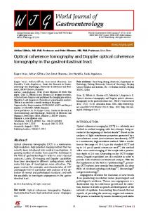
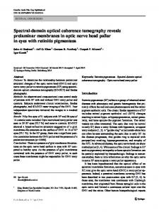
Clearly θ and δ control the radius of the Poincar´e sphere and provide total (unit radius) time-space coherence when either δ = 1 or θ = π, and a reduced sphere radius implying only partial coherence otherwise. Spatial Mode Coherence Tomography: We have implemented a new experimental tomography procedure that is able to acquire complete information of an arbitrary unknown two-mode input state made from Ga and Gb . An arbitrary tr optical beam of the form in (13) is a good example. The experimental setup for this novel tr tomography is illustrated by Fig. 1. In the preparation stage, a spatial light modulator (SLM) is used to generate a specific transverse mode, i.e., Ein (r⊥ , t) = Ga (r⊥ )Fa (t). It is then sent through a Mach-Zehnder interferometer (MZI) with two ordinary 50/50 beam splitters. In Path 1 (P1), the statistical temporal amplitude Fa (t) is delayed with a translation stage (TS), while in Path 2 (P2), a Dove prism (DP1) oriented at π/4 is used to rotate the spatial mode Ga into Gb and a filter (F) is placed to adjust the path intensity. The output beam of the MZI is in exactly the form E(r⊥ , t) = Ga (r⊥ )Fa (t)+Gb (r⊥ )Fb (t), of which the
FIG. 1: Schematic experimental setup. Light field (13) is prepared with a spatial light modulator (SLM) and a modified Mach-Zehnder interferometer (MZI), where filter (F) controls θ and the translation stage (TS) manages δ and φ. The Stokes parameters are measured with different combinations of a mode converter (MC), a Dove prism (DP2), and a MachZehnder interferometer with an additional Mirror (MZIM).
normalized expression is given by Eq. (15). The coefficients cos(θ/2) and sin(θ/2) are controlled by the filter in P2 and the parameters δ and φ are managed by adjusting the delay in P1. The tr coherence tomography stage is composed of three major elements, a spatial mode converter (MC), a Dove prism (DP2), and a Mach-Zehnder interferometer with an additional mirror (MZIM) [20]. These elements are respectively exact analogs of a quarter-wave plate, half-wave plate, and polarizing beam splitter that are employed in ordinary st or sr spin-polarization tomography. The mode converter MC contains a pair of appropriately separated cylindrical lenses that will introduce a relative i phase to the Gb mode with respect to Ga [21]. The Dove prism is used to rotate the spatial modes Ga and Gb to a desired basis αGa + βGb . The MZIM is employed to project the mode states Ga , Gb onto the two output ports respectively. With the combination of the MZIM and the Dove prism DP2 (oriented appropriately in the rotated basis, Ga , Gb and Ga ± Gb ), we are able to obtain the Stokes parameters S0 , S1 , and S2 . Accordingly, the combination of all three elements, with the DP2 and MC adjusted to account for a rotated basis Ga ± iGb , amounts to an effective measurement of S3 . Therefore all four Stokes parameters can be recorded. The conventional presentation of spatial modes for an optical beam is to display irradiance images of the transverse plane. These provide a positive visual validation of mode quality, but with the experimental setup described we can do much more. We produced and reconstructed the states of various tr “polarized” states. Fig. 2 displays the full Poincar´e sphere in panel (a) for all the generated states. One notes that all the linear states live on the
4 (a)
1.0
1.0
(b)
(c)
0.5
0.5
0.0
0.0
-0.5 -1.0 -1.0
-0.5 -0.5
0.0
0.5
1.0
-1.0 -1.0
-0.5
0.0
0.5
1.0
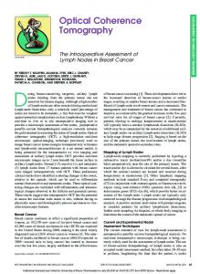
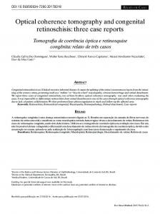
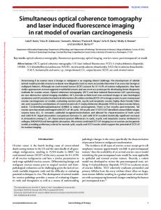
FIG. 2: Experimental data of various time-space polarization states. Plot (a) is a Poincar´e sphere representation of all measured states where the blue dots, black triangles and red squares denote linear, elliptical (including circular) and partial (including completely un-polarized) polarization states respectively. Plot (b) shows points on the equatorial plane S3 = 0, and it contains all the linear tr states. Plot (c) shows points in the S1 = 0 plane where the black upward triangles, black downward triangles, and red squares denote elliptical, circular and partially coherent tr states, respectively. The red dotted curve is the logarithmic polar spiral function δ = e−0.23φ tracking states with smaller and smaller degrees of tr coherence. Note: the error bars of the measured Stokes parameters are relatively small and not shown, but the magnitude of the maximum error is given in Table I.
S3 = 0 plane, as shown in (b), and all the elliptical and circular states live on the S1 = 0 plane and off the equator (i.e., S3 6= 0 or φ 6= nπ) as shown in panel (c). We also examined tr states intermediate between the pure t and r degrees of freedom. We prepared and measured eight different tr states of partial coherence by varying the amplitude correlation γ in the preparation stage of our apparatus. These states are located inside the tr Poincar´e sphere and are illustrated in both panels (a) and (c). One notes that with the decrease of the two-path temporal coherence δ combining with the relative phase φ change, the partially coherent states are gradually rotating into the center of the Poincar´e sphere, where there is a complete lack of coherence. That is, the degree of tr coherence is getting smaller and smaller. This sequence is shown explicitly in panel (c), and eventual nearness to the sphere center is quantified as Ptr = 0.050 in the bottom line of Table I below.
Summary: We have identified the tr category of optical coherence for the first time, and have described its features theoretically, and recorded those features experimentally. It is the missing member of a fundamental triad, previously completely hidden and now revealed by our derivation of the triad of coherence constraints. The members of the triad arise as in (3)-(5) from separate projections of the same optical field (1) on its three degrees of freedom. One member is traditionally identified with the correlation of temporal amplitude with spin (ordinary polarization). Another member has only recently been identified as a hidden coherence that correlates spatial amplitude with spin. The new third member is the first optical coherence independent of spin, and arises from correlation of temporal and spatial amplitudes. Our approach establishes that there can be no more hidden optical coherences [11]. The theoretical analysis leading to the discovery of the tr coherence domain revealed the presence of a quantitative balance between the degree of polarization and degree of entanglement (nonseparability) of the participating vector spaces (degrees of freedom). This balance takes the form of quadratic constraints applying to all pairs of degrees of freedom previously discussed. These constraints P 2 + C 2 = 1, have been interpreted as a new expression of complementarity [22], and we promised experimental confirmation of the third one. This has been done, as recorded in the final column of Table I below, 2 2 showing values for Ptr + Ctr equal to 1 well within the recorded standard deviation of 0.042 for the Stokes parameters of all five rows in the Table. Experimental entry into the domain of the third coherence required creation in the laboratory of a new form of optical coherence tomography, which we described in detail. It is of some interest to note that, as illustrated in Fig. 1, we are able to prepare arbitrary states of the form (15) by experimental choices of δ, θ and φ. Measurements of the parameters θ and δ can be realized by registering individual as well as combined intensities of P1 and P2 at the preparation stage after passing through an appro-
l c e p u
θ 3π/2 π/2 π/2 π/2 π/2
φ
S1 0 0.026 −π/2 0.029 π/4 0.024 5π/4 0.052 2π 0.042
S2 −0.916 −0.026 0.679 −0.271 −0.025
S3 0.037 −0.889 0.625 −0.306 −0.013
Ptr 0.918 0.890 0.923 0.307 0.050
2 2 Ctr Ptr +Ctr 0.392 0.996 0.455 0.998 0.384 0.999 0.945 0.988 0.991 0.985
TABLE I: Stokes parameters normalized to S0 , degree of tr “polarization” and concurrence for selected measured states. The first three are (l)inear, (c)ircular and (e)lliptical tr states described by different parameters of θ and φ, and the last two are (p)artial and (u)n-polarized states. The maximum standard deviation of all Stokes parameter measurements (including those not listed in the table but illustrated in Fig. 2) is 0.042.
5 priately rotated (45 degree) Dove prism. This process is independent of the subsequent coherence tomography procedure, and gives a measurement of Ctr independent of the measurement of Ptr , using the same modes. Finally we comment on the term “hidden”. Our discovery of the third coherence in the fundamental triad clarifies the issue of hidden coherences, which are a consequence of the intrinsically contextual character of coherence. Context matters! Coherence between two degrees of freedom is isolated by projection of the other independent degrees of freedom. A projection that produces such isolation to obtain the context for a specific pairwise coherence must automatically exclude (i.e., make “hidden”) any coherences that are associated to all other contexts, all other coherences. As soon as one of the three is made accessible by an appropriate experimental projection, the other two are automatically inaccessible, i.e., become hidden, even if present in the unprojected field. Acknowledgement: Support is acknowledged from a University of Rochester Research Award, ARO W911NF-14-1-063, ONR N00014-14-1-0260, as well as NSF grants PHY-1203931, PHY-1505189, and INSPIRE PHY-1539859.
∗ Electronic address:
[email protected] [1] Th. Young, Phil. Trans. Royal Soc., London xcii 12, 387 (1802). [2] See, for example, R.J. Glauber, “Optical Coherence and Photon Statistics”, in Quantum Optics and Electronics C. deWitt, et al., Eds., (Gordon and Breach, New York, 1964) [3] L. Mandel and E. Wolf, “Optical Coherence and Quantum Optics” (Cambridge Univ. Press, 1995). [4] K.H. Kagalwala, G. di Giuseppe, A.F. Abouraddy and B.E.A. Saleh, Nat. Phot. 7, 72 (2013). [5] A particularly wide-ranging examination is provided by F. de Zela, Phys. Rev. A 89, 013845 (2014). [6] J.H. Eberly, Contem. Phys. 56, 407 (2015). [7] J. Svozil´ık, A.Vall´es, J. Peˇrina, Jr., and J.P. Torres, Phys. Rev. Lett. 115, 220501 (2015). [8] W. F. Balthazar, C. E. R. Souza, D. P. Caetano, E. F. Galv˜ ao, J. A. O. Huguenin, A. Z. Khoury, arXiv:1511.02265 (2015).
[9] J.H. Eberly, Xiao-Feng Qian, Asma AlQasimi, Hazrat Ali, M.A. Alonso, R. Guti´errez-Cuevas, Bethany J. Little, John C. Howell, Tanya Malhotra and A.N. Vamivakas, “Quantum and Classical Optics – Emerging Links”, Phys. Scrip. 91, 063003 (2016). [10] A complete orthonormal set of time functions directly determined by the random process itself can be obtained as eigenfunctions of the integral equation in which the kernel is the random signal’s autocorrelation function. See M. Kac and A.J.F. Siegert, Ann. Math. Stat. 18 438442 (1947). [11] We take the three degrees of freedom and their projections as exhaustive just for convenience. The transverse coordinate contains two degrees of freedom that could be treated separately, and a beam that is split to follow independent trajectories can allow each path to be counted separately (see R.J.C. Spreeuw, Phys. Rev. A 63, 062302 (2001) and Khoury, et al. [8]). These additional degrees of freedom provide only a few additional contexts. [12] See E. Wolf, N. Cim. 13, 1165 (1959), as well as a comprehensive modern overview in Introduction to the Theory of Coherence and Polarization of Light, E. Wolf (Cambridge Univ. Press, 2007). [13] C. Brosseau, Fundamentals of Polarized Light: A Statistical Optics Approach (Wiley, New York, 1998). [14] W. K. Wootters, Phys. Rev. Lett. 80, 2245 (1998). [15] The constraint also appears in the context of qutrits and ququarts: M.V. Fedorov, P.A Volkov, J.M. Mikhailova, S.S. Straupe and S.P. Kulik, New J. Phys. 13, 083004 (2011). [16] F. Gori, M. Santarsiero, and R. Borghi, Opt. Lett. 31, 858-860 (2006). See also F. Gori, M. Santarsiero, S. Vicalviddag, R. Borghi and G. Guattari, Opt. Lett. 23, 241 (1998). [17] The original paper is: E. Schmidt, “Zur Theorie der linearen und nichtlinearen Integralgleichungen. 1. Entwicklung willk¨ uriger Funktionen nach Systeme vorgeschriebener”, Math. Ann. 63, 433 (1907). For background, see M.V. Fedorov and N.I. Miklin, “Schmidt modes and entanglement”, Contem. Phys. 55, 94 (2014). [18] X.-F. Qian and J.H. Eberly, Opt. Lett. 36, 4110 (2011). [19] M. J. Padgett and J. Courtial, Opt. Lett. 24, 430 (1999). [20] H. Sasada and M. Okamoto, Phys. Rev. A 68, 012323 (2003). [21] M.W. Beijersbergen, L. Allen, H.E.L.O. van der Veen and J.P. Woerdman, Opt. Commun. 96, 123 (1993). [22] This form of complementarity deserves further attention. See X.-F. Qian, M.A. Alonso and J.H. Eberly, Quantum Electronics FTu2F.5, Frontiers in Optics Conference (San Jose CA, 2015).