David Stern. Thore Graepel .... Philipp Hennig, David Stern, Thore Graepel g0 g1 g11 v11 ..... a 'sweet spot' between unstructured priors and non- probabilistic ...
Coherent Inference on Optimal Play in Game Trees
Philipp Hennig Cavendish Laboratory 19 J J Thomson Avenue Cambridge CB3 0HE, UK
David Stern Microsoft Research Ltd. 7 J J Thomson Avenue Cambridge CB3 0FB, UK
Abstract Round-based games are an instance of discrete planning problems. Some of the best contemporary game tree search algorithms use random roll-outs as data. Relying on a good policy, they learn on-policy values by propagating information upwards in the tree, but not between sibling nodes. Here, we present a generative model and a corresponding approximate message passing scheme for inference on the optimal, off-policy value of nodes in smooth and/or trees, given random roll-outs. The crucial insight is that the distribution of values in game trees is not completely arbitrary. We define a generative model of the on-policy values using a latent score for each state, representing the value under the random roll-out policy. Inference on the values under the optimal policy separates into an inductive, pre-data step and a deductive, post-data part. Both can be solved approximately with Expectation Propagation, allowing off-policy value inference for any node in the (exponentially big) tree in linear time.
1
Introduction
Many round-based two-player games, like Chess and Go, can be represented, up to transpositions, by graphs with the structure of and/or trees (Nilsson, 1971). If the branching factor b is constant, a tree of depth d contains bd nodes. For Go, b and d are on the order of 200, so it seems finding the optimal path through the game should be intractable. Yet humans can find good paths through the Go tree in finite time. Appearing in Proceedings of the 13th International Conference on Artificial Intelligence and Statistics (AISTATS) 2010, Chia Laguna Resort, Sardinia, Italy. Volume 9 of JMLR: W&CP 9. Copyright 2010 by the authors.
Thore Graepel Microsoft Research Ltd. 7 J J Thomson Avenue Cambridge CB3 0FB, UK
A crucial property of games that humans use is that the tree has structure: Winning positions are not randomly distributed among the tree’s leaves, but clustered. This structure can be modeled by a latent score, representing the amount by which one player is ‘ahead’ or ‘behind’. Random play leads to a random walk, typically changing the evaluation by small increments. Critical moves, changing the score drastically, are a rare occurrence in the tree overall. Although it is not usually mentioned explicitly, this smoothness is a crucial intuition behind Monte Carlo algorithms for ‘best first’ tree search, like UCT (Kocsis and Szepesv´ari, 2006), which have been very successful recently. These algorithms repeatedly play roll-outs— random descents through the tree to a leaf, generated by a relatively weak or uniformly random policy. The search tree is expanded asymmetrically from the root, based on the frequency of wins and losses in the rollouts. If wins and losses were distributed uniformly at random among the leaves, the roll-out results would be almost completely uninformative (Pearl, 1985). The best contemporary Go machines are using UCT as part of their method (Gelly and Silver, 2008). However, UCT-like methods base their value estimates directly on average outcomes of tree-descents, making them dependent on a good exploration and roll-out policy. They also do not propagate information laterally in the tree, although, thanks to the smoothness of the tree, the value of a node does contain information about the value of its siblings. In this paper, we construct an explicit generative model for the value of game tree nodes under the random roll-out policy. Finding the value under the optimal policy would amount to solving a min-max optimization problem of complexity O(bd ) if all nodes were observed. However, for best-first search algorithms, we will show how an approximate closed form for the unobserved parts of the tree can be constructed and used to derive an approximate message passing scheme. The resulting algorithm tracks a joint posterior belief over the optimal values of all nodes in the
326
Coherent Inference on Optimal Play in Game Trees
tree. It incorporates a new roll-out at depth k from the root in O(kb) time (using heuristics, this can be brought to O(k), the complexity class of UCT), arriving at an intermediate set of local marginals which is sufficient to evaluate the posterior of an arbitrary node at depth ` in the tree (something classic Monte Carlo algorithms cannot do) with cost O(`). The algorithm can be interpreted as an instance of Bayesian off-policy reinforcement learning (Watkins and Dayan, 1992; Dearden et al., 1998), inferring the optimal policy from samples generated by a non-optimal policy. Our method might be applicable, to varying degree, to other tree-structured optimization problems, if they exhibit a functional relationship between steps; c.f. the metric (though not tree-structured) sets of bandits considered by Kleinberg et al. (2008).
the tree. The only type of data available (at request) is the length ` ∈ N and result ri ∈ {−1; 1} of random roll-outs of the game starting at node i. A roll-out is a path through the tree to a terminal node, generated by a policy choosing stochastically (not necessarily uniformly) among available moves in each encountered position. (The policies of contemporary UCT algorithms do not choose moves uniformly at random. See Section 3.4 for experimental evidence that our model can still be approximately valid in this case.)
Our main contributions are the generative model for the score of game positions, the formulation of a probabilistic best-first tree search algorithm, and a demonstration of Expectation Propagation on min-max trees (the necessary mathematical derivations are part of a technical report by one of the authors (Hennig, 2009)).
Definition: The score gi of node i models the value of i under random play. It is a real number such that
2.2
The following two definitions jointly form a generative model M for the latent scores G = {gi } and optimal values V = {vi } of tree nodes i.
• for any terminal position t, sign(gt ) = rt , where rt is the binary result of the game at t. The likelihood for gt is thus a step function (denoted θ):
Probabilistic approaches to game tree search have been suggested before (see e.g. Baum and Smith, 1997; Russell and Wefald, 1991; Palay, 1985; Stern et al., 2007). These works concentrated on guiding the search policy. Here we focus on efficient and consistent off-policy inference for the entire tree. This is valuable because a coherent posterior over off-policy values provides meaningful probabilistic training data for Bayesian algorithms attempting to learn a generalizing evaluation function based on features of the game state.
2
Methods
This section defines the problem (2.1), then develops the algorithm in several steps. We define the generative model of on-policy and off-policy values (2.2), show how to perform inference in this model by way of example (2.3), and finally combine the results into an explicit algorithm (2.4). 2.1
The task is to predict the outcome of the game, assuming optimal play by both players, from any position in 1
p(rt |gt ) = θ(rt gt )
Games with real-valued outcomes are in fact an easier variant of this problem, because the scores gt of terminal nodes can be observed directly, rather than just their signs.
(1)
• the score of child node c of node i is generated from gi by a univariate Gaussian step: p(gc |gi , M) = N (gc ; gi , 1)
(2)
• the prior for the score of the root note is Gaussian p(g0 ) = N (µ0 , σ02 ) (one is free to choose µ0 and σ0 , although µ0 = 0 is the obvious choice). Thus, scores of sibling nodes are independent given their parent’s score, and roll-outs are Brownian random walks. For binary results, the scale factor of the steps is arbitrary and set to 1 for simplicity only. Definition: The off-policy value vi of node i is the value of node i under optimal play by both players. That is • for terminal positions t, we have vt = gt .
Problem Definition
We consider a tree-structured graph defining a roundbased, loop-free, zero-sum game between two opposing players, max and min with binary1 outcomes 1 and −1 (“win” and “loss” from max’s point of view). max is defined to be the first player to move.
Generative Model
• for non-terminal positions i with children {c}i ( maxc {vc } if max plays at i vi = (3) minc {vc } if min plays at i. We note in passing that or-trees (i.e. tree-structured optimization problems, and non-adversarial games like Solitaire) are a trivial variant of this formulation. Figure 1 shows the full generative model for a small tree of b = 2 and d = 4, as a directed graphical model. Note that only the sign of outcomes is observed (black nodes), all other variables are latent.
327
Philipp Hennig, David Stern, Thore Graepel
N( g1 ∼
g1
ou
t
g11
g0
g2 ∼ N(
g0 , 1)
max
g2
g12
g21
g22
min
nodes stored in memory
max
rol l
G
g0, 1)
min Terminal Position
R
untracked nodes (inductive part)
min V
v11
v12
v21
v1
v0 = max(v1 , v2 )
v1 = min(v11 , v12 )
v0
v22
max
optimal value (ground truth)
min
v2
max
Figure 1: Generative model (Bayesian network) for the scores G, the roll-out results R and the optimal values V of an example game represented by a binary tree of depth 4. Shown is the situation after four search-descents into the tree. The most recent roll-out (of length 2) is shown as two black curved arrows. Ground truth generation of v as thick arrows (i.e. optimal play consists of max moving from node 0 to node 1, then min moving to 12, etc.). Note that, while the v nodes are shown below the g nodes here for readability, in the text ‘up’ and ‘down’ refer to the game tree structure, with parent nodes vi being ‘above’ children vij . 2.3
Inference
We will derive an approximate Belief Propagation algorithm (Lauritzen and Spiegelhalter, 1988; Pearl, 1988) to perform inference both on the scores and values, using Gaussian Expectation Propagation (Minka, 2001) to project the messages to the normal exponential family. Belief Propagation is a message passing scheme between the nodes of a Bayesian network: The marginal probability p(xi ) of a latent variable xi in the model is the product of messages mxj (xi ) from neighboring variables xj , as defined by the structure of the graph. Gaussian Expectation Propagation keeps inference tractable by replacing these messages with approximate Gaussian messages, such that the resulting marginal matches the first two moments of the true marginal. Inspecting Figure 1, it might seem like inference in the tree would call for messages among all bd nodes. In this Section, we will show that this can be avoided, because the messages from unobserved parts of the tree can be derived a priori, in jointly O(bd) time. We assume the learner acquires data in a best-first manner: At any given point in time, it tracks an asymmetric but contiguous tree in memory which includes the root. Additional nodes are added to the boundary of the stored tree by requesting a roll-out from that
node. The message passing is performed in parallel with the search process. The resulting message passing schedule is quite complex. For clarity, we will use an example descent through Figure 1. 2.3.1
On-Policy Inference on g
Each search descent begins at the root node 0. As the descent passes through the tracked part of the tree, a policy π chooses among available children, potentially based on the current beliefs over their v. For our example, say the policy chose the descent 0 → 1 → 12. At each step, we update the message from the current node to the chosen child. The message out of g1 in the direction of g12 is Y 2 mpa(1) (g1 ) mgj (g1 ) ≡ N (µ1\12 , σ1\12 ) (4) j∈ch(1)\12
where ch(1)\12 is the set of child nodes of 1 excluding node 12, and pa(1) is the parent node (i.e. 0) of 1. And the message into g12 is Z mg1 (g12 ) = p(g12 |g1 )p(g1 |gpa(1) , {gch(1)\12 }) dg1 2 = N (µ1\12 , σ1\12 + 1)
(5) Assume node 12 just reached is not part of the stored tree yet. To add it to the tree, we request a roll-out
328
Coherent Inference on Optimal Play in Game Trees
starting from 12, which turns out to be of length ` = 2 and have result r = +1 (see Figure 1). The data thus gained is a likelihood p(r|gt ) of the score of the terminal position t at the end of the roll-out, which is a step-function and thus not normalizable. However, we can generate a prior over gt as a message from the current marginal over g12 by integrating out the ` intermediate steps (see Equation (5)): 2 p(gt |g12 ) = N (µ12 , σ12 + `)
(6)
giving a posterior over gt which is a truncated Gaussian. To get the EP message back to g12 , we need EP a function ftrG , which calculates the moments of this truncated Gaussian distribution. The calculation is straightforward, because for Gaussians in general Z ∞ �µ� �µ� + σφ and xN (x; µ, σ 2 ) = µΦ σ σ 0 Z ∞ �µ� �µ� x2 N (x; µ, σ 2 ) = (µ2 + σ 2 )Φ + µσφ σ σ 0 This result was used previously for EP by Herbrich et al. (2007). To finally arrive at the message mr12 (g12 ) from the roll-out to g12 , we need to apply fN (0,`) again to the resulting EP message. Note that the message contains no g other than gi . It is thus possible to perform inference on gi using exactly two messages: One from its parent node, and one from the outcome of the roll-out. To incorporate the new knowledge from this roll-out into all parent nodes of g12 , we pass messages of analogous form to Equation (5) back up the tree. This obviously does not propagate the information through the whole tree, but it leads to a situation where the score gi of any node i in the tree can be evaluated in linear time, simply by performing one descent from the root towards i, updating messages analogously to Equation (5) downwards during the descent. There is one more pitfall to avoid: The next time a search descent passes through node 12 which currently lies at the boundary of the tracked tree, leading to the addition of a child node of 12 and a roll-out from there, it becomes necessary to remove the information gained from the roll-out at node 12 from the marginal. Because the roll-out necessarily passed through one of i’s children, information from that child would otherwise be counted twice. This removal corresponds to ‘dividing’ the corresponding message out of the marginal, which for Gaussians has closed form: N (x; µa , σa2 )/N (x; µb , σb2 ) ∝ � � � � � � µa µb −2 −1 −2 −1 −2 −2 N x; − σ − σ , σ − σ a a b b σa2 σb2 This ‘division’ operation for distributions is used extensively in EP message passing schemes because it increases computational efficiency (Minka, 2001).
2.3.2
Off-Policy Inference on v
The previous paragraph sketched the message passing inference leading to a consistent posterior over scores G. How can these beliefs be used to obtain a posterior over the values V ? We will use the definitions of Section 2.2 to again derive a message-passing scheme running parallel to the search process. First, consider again node i = 12 in Figure 1, at the boundary of the stored tree. The value under optimal play is the sum of the two independent variables vi = gi + ∆i
(7)
where ∆i is the optimal reachable increment to the score of i. So the inference breaks up into a deductive part (on gi , as solved in the previous section) and an inductive part (on ∆i ). If the next move after i is controlled by max (replace max with min in the opposite case), then ∆i =
max j∈children(i)
{ξj + ∆j }
(8)
where ξj ∼ N (0, 1) is the unknown Brownian step to the score of node j. Deriving a belief over ∆i for any node i, which is `i steps from a terminal position, is a recursive problem which depends only on `i and the branching factor b: Assuming min gets the last move (with straightforward variations in other cases), ∆i is δ(∆i − 0) (9) ∆i (`i , b) = maxj=1...b {∆j (`i − 1, b) + ξj } minj=1...b {∆j (`i − 1, b) + ξj } for ` = 0, for ` mod 2 = 0 and for ` mod 2 = 1, respectively. Similarly to the situation in the previous Section, the beliefs generated by this recursive operation are not Gaussian themselves. To perform the EP approximaEP tion, we need the function fmax / min calculating the moments of the maximum or minimum over Gaussian variables. The necessary derivations are lengthy and thus left out here for brevity. A technical report by one of the authors (Hennig, 2009) develops these moments for the case of the maximum of two Gaussian variables (Equation 25 in the cited work) and shows how to combine such binary comparisons iteratively into an approximate posterior belief over the maximum of a finite set of such variables (Section 3.2 in the cited work). The corresponding messages for the minimum of variables is a trivial variant, because mini {xi } = − maxi {−xi }. Using this approximation, we arrive at a recursive operation in closed form, which can be used to derive the message from ∆(`) for all ` up to a pre-defined depth. This can be done prior
329
Philipp Hennig, David Stern, Thore Graepel
to data acquisition, once for the entire game tree, in O(bd) time, which is easily tractable even for massive game trees like that of 19 × 19 Go. In our simple, non-optimized implementation, this step takes about 2 minutes on a contemporary desktop machine, for a tree of Go-like dimensions (10400 nodes). This step is a parametrized version of the Monte Carlo technique known as density evolution (e.g. MacKay, 2003, Sec. 47.5). See Section 3.3 for an experimental analysis of the quality of the approximation. We sum the independent variables gi and ∆i , using the exact function � � fP N N (µa , σa2 ), N (µb , σb2 ) = N (µa + µb , σa2 + σb2 ) For a node j which does not lie on the boundary of the stored tree, vj is given by Equation (3). Marginals p(vcj ) are available for all children cj of j in this case. Hence, an approximate Gaussian message to vj from its children can be found using the same method as above. However, it is important to note that the children of vj are correlated variables, because they are all of the form shown in Equation (7), sharing the contribution gj . The EP equations derived in (Hennig, 2009) include the correlated case. Using approximate Gaussian messages 2 q(vk ) = N (µk , σk2 ) = N (µgj + µ∆k , σg2j + σ∆ ) (10) k
for each child k of j, the correlation coefficient2 ρk1 k2 between two children k1 and k2 is ρ12 = V −1 (σg2i − µgi µ∆k1 − µgi µ∆k2 − µ∆k1 µ∆ik2 ) 2 V ≡ (σg2i + σ∆ − 2µgi µ∆k1 )1/2 k 1
2 · (σg2i + σ∆ − 2µgi µ∆k2 )1/2 k 2
2.3.3
Loopiness
From Figure 1, it is clear that the graphical model contains loops. However, because we assume no outside information on the optimal value v0 of the root, the EP messages from the v’s to the g’s are uniform (Hennig, 2009). So inference on the g’s is not influenced by the v-part of the graph. Thus, while the inclusion of the v-nodes does create loops in the overall graph, the message-passing within the v-part of the tree is based on a consistent set of marginals on the g’s. 2.4
Algorithm
Algorithm 1 sums up the message-passing and search scheme presented in the previous Sections. It defines a recursive function that descends through the tracked 2
The correlation coefficient ρij betweenptwo Gaussian variables i and j is defined by cov (ij) = ρij var (i) var (j).
tree to a leaf, passing messages downward (the operator fN (0,1) (p) refers to Equation (5)). At the boundary of the stored tree, it performs a roll-out, then passes g and v messages upwards to the root. The actual top-level search algorithm repeatedly calls this function, accumulating more and more data, at roughly constant computational cost per call (apart from the small increase in cost caused by the growth of the stored tree). The descent through the stored tree is guided by some policy π, which may (and should) depend on the current beliefs over values v. The notation pa(i) and si(i) refers to the parent of i and the set of siblings of (and including) i, respectively. The function stored accesses a one-dimensional array of stored inductive messages from the un-explored parts of the tree, as discussed in Section 2.3.2. Algorithm 1 Bayesian Best-First Tree Search 1: procedure descent(i) 2: if i previously visited then 3: . choose child c to explore 4: c ← π(i) 5: . update message to c. 6: p(gc ) ← p(gc )/mgi (gc ) 7: mgi (gc ) ← fN (0,1) [p(gi )/mgc (gi )] 8: p(gc ) ← p(gc ) · mgi (gc ) 9: . continue descent (returns g message from child) 10: m0c (gi ) ← descent(c) 11: . update marginals 12: p(gi ) ← p(gi )/mc (gi ) · m0c (gi ) 13: mc (gi ) ← m0c (gi ) 14: else 15: . divide out roll-out from parent’s marginal 16: p(gpa(i) ) ← p(gpa(i) )/mrpa(i) (gpa(i) ) 17: mrpa (gpa(i) ) ← N (0, ∞) 18: . update message from parent to gi (lines 3 to 5) 19: . do roll-out 20: (ri , `i ) ← rollout(i) 21: . generate message from � EProll-out result to i � (ri , fN (0,`i ) [p(gi )]) 22: mri (gi ) ← fN (0,`i ) ftrG 23: p(gi ) ← p(gi ) · mri (gi ) 24: . generate marginal for vi 25: p(vi ) ← fP N [p(gi ),stored(`i )] 26: end if 27: . Calculate messages to parent’s g and v 28: mi (gpa(i) ) ← fN (0,1) (p(gi )/mpa(i) (gi )) EP 29: p(vpa(i) ) ← fmax / min ({p(vk )}k∈si(i) , p(gi )) 30: return mi (gpa(i) ) 31: end procedure
2.5
Exploration Policies
While the inference process itself is independent of the chosen policy π in Algorithm 1, the policy is crucial to make the roll-outs informative about the optimal path (this is a general feature of off-policy reinforcement learning). Many possible policies are available,
330
Coherent Inference on Optimal Play in Game Trees
value of gi under the model through � � Z ∞ gi N (gt , gi , `i ) dgt = Φ √ p(win|gi ) = `i 0
1.2 1.6 1.8 depth =1 depth =2 depth =3
log p(g;v)
®
1.4
2.0 2.2 100
101
102
ndescent
103
104
Figure 2: Log likelihood of the ground truth value of gi (crosses) and vi (triangles) under the beliefs of the model, at varying depth from the root in artificial trees. Averages over all nodes at those depths. among them the point-estimate based UCT (Kocsis and Szepesv´ ari, 2006), greedy choice among samples (Thompson, 1933), information gain (Dearden et al., 1998) and ‘optimistic’ exploration based on weighted sums of mean and variance of the value estimates. The latter approach has received some interest recently (Kolter and Ng, 2009), but the ‘right’ choice of policy is still a matter of open debate. In our experiments, we used optimistic exploration where applicable.
3
Results
We performed experiments to answer several questions arising with regard to the described inference model: Is the model of Brownian motion applicable for real games, like Go (3.1)? Is the EP approximation on the roll-out results effective (3.2)? Does the recursive min/max approximation in the inductive part of the inference produce a reasonable approximation of the true min/max values (3.3)? How robust is the model to mis-match between generative model and ground truth (3.4)? And could the algorithm be used as a standalone searcher (3.5)? 3.1
Structure of Go Game Trees
We generated one random path through the tree of 9 × 9 Go. At each level in this path, roll-outs from all legal moves i at this position were generated (1000 rollouts from each i). Depending on the depth from the root, there were between 81 and 0 such legal positions. We stopped the game after 71 steps, when there were less than 5 legal moves available. The average length `¯i of the roll-outs and the empirical frequency pˆ(win|i) of a win for the max player from i under a random roll-out policy was stored. This implicitly defines the
(11)
where we replace p(win|gi ) and `i with empirical averages. With sufficiently many samples, p(win|gi ) and thus gi can be evaluated up to negligible error. Our model M then amounts to the statement that the {gi } of sibling nodes in the tree are distributed like the standard normal distribution around their parent’s value. Figure 3 shows Q-Q plots of these empirical distributions against Φ for depths d = 0 to 71 from the root. A standard normal would lie on the diagonal in this plot; weaker tailed distributions are steeper, heavier tailed ones flatter. The left plot shows results from a uniform roll-out policy (only excluding illegal and trivially bad ‘suicide’ moves). Given the limited sample sizes, especially towards the end of the game, the empirical distributions are strikingly similar to Φ(x). Contemporary Monte Carlo search algorithms use ‘heavy roll-outs’, i.e. policies that produce less random, more informative results. Clearly, the hypothesis of ergodicity in our model will be more and more invalid the smarter the policy (the limit of a perfect policy would repeatedly generate only a single perfect roll-out). To examine how drastic this effect is, we repeated the above experiment with a smart policy, similar to the published parts of MoGo (Gelly et al., 2006) (Figure 3, right). While the results do develop heavier tails, the overlap with Φ(x) is still quite good. 3.2
Inference on the Generators
A good way to evaluate the quality of Bayesian models is the (log) likelihood they assign to ground truth in known test environments. To do so, we generated 500 artificial trees of b = 2, d = 18 from M. The inference model was implemented as presented in Algorithm 1. A time step corresponds to one descent into the tree, ending with a roll-out at a previously unexplored node. For the descent through previously visited nodes, an optimistic policy was used (see Section 2.5), choosing greedily among children i based on µvi + 3σvi . In addition, the value of the root node’s score was assumed to be 0 with high precision. Figure 2 shows the log likelihood assigned to the ground truth of both g and v at distances 1, 2 and 3 from the root. As expected, the likelihoods rise on average during learning. They saturate when the majority of the nodes is expanded, because the (binary) roll-out results do not contain sufficient information to determine g, and thus v, to arbitrary precision. Nodes deeper in the tree saturate at smaller likelihoods because they receive information from fewer offspring nodes. They
331
1.0
1.0
0.8
0.8
0.6
0.6
0.4
0.4
0.2
0.2
Z g
−∞
ˆp(g0 ) dg0
Philipp Hennig, David Stern, Thore Graepel
0.00.0
0.2
0.4
Φ(g)
0.6
0.8
1.0 0.00.0
0.2
0.4
Φ(g)
0.6
0.8
1.0
Figure 3: Quantile-quantile plot of 71 empirical distributions of g, centered on their mean, at varying depth from the root, for one random path through Go, against the standard normal distribution Φ(x) (black dotted line). Left: Random roll-out policy. Right: Smart roll-out policy. Color intensity of the plots decays linearly with depth from the root. Note that the distributions far from the root are based on increasingly small sample sizes.
0.6
b =5,` =6 b =5,` =5
0.5
repeated application of the Gaussian approximation to non-Gaussian beliefs, there is good agreement between predictions and ground truth.
p(∆)
0.4 0.3
3.4
0.2
For the last two experiments, the artificial game trees were generated by the generative model M, and we showed in Section 3.1 that the real-world game Go is in fact pretty close to this model. However, other games might be less well approximated by M. As a tentative test of the severity of the errors thus introduced, the Bayesian searcher was tested on 500 generated p-game trees (Kocsis and Szepesv´ari, 2006) with b = 2, d = 18. These trees are also generated by a latent stochastic variable, but with a different generative model, choosing ξi uniformly from [−1, 0] if the player is min and uniformly from [0, 1] if the player is max.
0.1 0.0
4
2
0 ∆
2
4
Figure 4: Empirical histogram and model predictions (lines) for the optimal future value increment ∆ (see Equation (7)), for p(∆|` = 6, b = 5) (first move for max, last move for min) and p(∆|` = 5, b = 5) (first and last move for min). Model predictions as lines. also start out with a smaller likelihood because their priors contain more uncertainty. Note that the message passing causes the beliefs to develop simultaneously at all three depths, even though the nodes at greater depths are not explored until several descents after initialization. 3.3
Errors Introduced by Model Mismatch
We performed a best-first search in these trees (results not shown due to lack of space), and compared to the performance on trees for which M is the correct model. The performance on these two types of trees during the search was very similar, except for a globally slightly higher chance of the model misclassifying nodes into winning and losing nodes. At least in this particular case, the model mismatch causes only minor decay in performance.
Recursive Inductive Inference on v 3.5
To evaluate the quality of the inductive part of the approximation, 1000 artificial game trees were generated and solved by explicit min/max search as in the preceding section. Figure 4 compares empirical ground truth of ∆ and values predicted by pre-data inference, for all nodes at two different distances ` from the leaves, in 1000 artificial game trees. Despite the
Use as a Standalone Tree Search
It is tempting to interpret the presented inference algorithm as a standalone search method. Experiments on artificial game trees (results not shown) suggest that the resulting algorithm is rarely much better at exploring the tree than e.g. a vanilla UCT searcher, and that performance depends strongly on the policy used. The
332
Coherent Inference on Optimal Play in Game Trees
intent of the presented algorithm is not to develop a good tree searcher, but to provide a consistent posterior from which generalizing evaluation functions can be learned.
4
Conclusion
We have presented a generative model for game trees, and derived an approximate message-passing scheme for inference on the optimal value of game positions, given samples from random roll-outs. Inference separates into two tractable deductive and inductive parts, and allows evaluation of the marginal value of any node in the tree in linear time. Similar to the way humans think about games, the computational cost of our algorithm depends more directly on the number of data collected than on the size of the game tree. Like any model, the assumption of Brownian motion is imperfect. Neither does it catch all the details of any one game, nor does it necessarily apply to all games. But it provides a quantitative concept of a smoothly developing game between competing players. Our experimental results suggest that errors introduced by model mismatch are not severe, and that this is a strikingly good model of Go. We argue that it lies at a ‘sweet spot’ between unstructured priors and nonprobabilistic, rule-based methods, which can over-fit. Retaining a posterior does not necessarily improve on point-based methods in the search for the optimal next move. Nevertheless, the results presented here are valuable in two ways: humans use sophisticated feature-based concepts to play games, not full tree search. Emulating this behavior with a Bayesian algorithm, learning an evaluation function of features of the game position, requires probabilistic beliefs over the optimal values, which our algorithm provides, decoupling the task of designing an evaluation function from that of data acquisition. Secondly, game trees are discrete planning tasks (hierarchical bandit problems). Our results indicate that such problems can exhibit structure (in this case, correlation) even if they might ostensibly look unstructured, offering potential for considerable performance increase. Acknowledgements The authors would like to thank Carl Scheffler, David MacKay and the anonymous reviewers for helpful discussions and comments. This work was supported by a grant from Microsoft Research Ltd.
References E.B. Baum and W.D. Smith. A Bayesian approach to relevance in game playing. Artificial Intelligence, 97(1-2):
195 – 242, 1997. R. Dearden, N. Friedman, and S. Russell. Bayesian Qlearning. In Proc. AAAI Conference on Artificial Intelligence, pages 761–768, 1998. S. Gelly and D. Silver. Achieving master level play in 9x9 computer Go. In Proc. AAAI Conference on Artificial Intelligence, pages 1537–1540, 2008. S. Gelly, Y. Wang, R. Munos, and O. Teytaud. Modification of UCT with patterns in Monte-Carlo Go. Research Report RR-6062, INRIA, 2006. P. Hennig. Expectation propagation on the maximum of correlated normal variables. arXiv:0910.0115 [stat:ML], October 2009. R. Herbrich, T. Minka, and T. Graepel. TrueSkill: A Bayesian skill rating system. NIPS, 20:569–576, 2007. R. Kleinberg, A. Slivkins, and E. Upfal. Multi-armed bandits in metric spaces. In Proc. ACM Symposium on Theory of Computing, pages 681–690, 2008. L. Kocsis and C. Szepesv´ ari. Bandit based Monte-Carlo planning. In Proc. European Conference on Machine Learning, pages 282–293. Springer, 2006. J.Z. Kolter and A.Y. Ng. Near-Bayesian exploration in polynomial time. In Proc. International Conference on Machine Learning, volume 26, 2009. S. L. Lauritzen and D. J. Spiegelhalter. Local computations with probabilities on graphical structures and their application to expert systems. J. Royal Statistical Society, 50:157–224, 1988. D.J.C. MacKay. Information theory, inference, and learning algorithms. Cambridge Univ. Press, 2003. T.P. Minka. Expectation Propagation for approximate Bayesian inference. In Proc. Uncertainty in Artificial Intelligence, volume 17, pages 362–369, 2001. N.J. Nilsson. Problem-solving methods in artificial intelligence. McGraw-Hill Pub. Co., 1971. A.J. Palay. Searching with probabilities. Pitman Pub., Inc., 1985. J. Pearl. Heuristics: intelligent search strategies for computer problem solving. Addison-Wesley, 1985. J. Pearl. Probabilistic reasoning in intelligent systems. Morgan Kaufmann, 1988. S. J. Russell and E. Wefald. Do the Right Thing. MIT Press, 1991. D. Stern, R. Herbrich, and T. Graepel. Learning to solve game trees. In Proc. International Conf. on Machine Learning, volume 24, pages 839–846. ACM, 2007. W.R. Thompson. On the likelihood that one unknown probability exceeds another in view of two samples. Biometrika, 25:275–294, 1933. C.J.C.H. Watkins and P. Dayan. Technical note: Qlearning. Machine Learning, 8:279 – 292, 1992.
333