Coherent Processing Across Multiple Staggered Pulse Repetition ...

AFRL-SN-RS-TR-2004-43 Final Technical Report February 2004

COHERENT PROCESSING ACROSS MULTIPLE STAGGERED PULSE REPETITION INTERVAL (PRI) DWELLS IN RADAR Syracuse University

APPROVED FOR PUBLIC RELEASE; DISTRIBUTION UNLIMITED.

AIR FORCE RESEARCH LABORATORY SENSORS DIRECTORATE ROME RESEARCH SITE ROME, NEW YORK

STINFO FINAL REPORT This report has been reviewed by the Air Force Research Laboratory, Information Directorate, Public Affairs Office (IFOIPA) and is releasable to the National Technical Information Service (NTIS). At NTIS it will be releasable to the general public, including foreign nations.

AFRL-SN-RS-TR-2004-43 has been reviewed and is approved for publication.

APPROVED:

/s/ DAVID B. BUNKER Project Engineer

FOR THE DIRECTOR:

/s/ RICHARD G. SHAUGHNESSY, Lt. Col., USAF Chief, Rome Operations Office Sensors Directorate

Form Approved OMB No. 074-0188

REPORT DOCUMENTATION PAGE

Public reporting burden for this collection of information is estimated to average 1 hour per response, including the time for reviewing instructions, searching existing data sources, gathering and maintaining the data needed, and completing and reviewing this collection of information. Send comments regarding this burden estimate or any other aspect of this collection of information, including suggestions for reducing this burden to Washington Headquarters Services, Directorate for Information Operations and Reports, 1215 Jefferson Davis Highway, Suite 1204, Arlington, VA 22202-4302, and to the Office of Management and Budget, Paperwork Reduction Project (0704-0188), Washington, DC 20503

1. AGENCY USE ONLY (Leave blank)

2. REPORT DATE

3. REPORT TYPE AND DATES COVERED

FEBRUARY 2004

Final Jan 97 – Jun 01

4. TITLE AND SUBTITLE

5. FUNDING NUMBERS

COHERENT PROCESSING ACROSS MULTIPLE STAGGERED PULSE REPETITION INTERVAL (PRI) DWELLS IN RADAR

C PE PR TA WU

6. AUTHOR(S)

Tapan K. Sarkar and Jinhwan Koh

7. PERFORMING ORGANIZATION NAME(S) AND ADDRESS(ES)

- F30602-97-C-0041 - 62204F - 4506 - 11 - PE

8. PERFORMING ORGANIZATION REPORT NUMBER

Syracuse University Office of Sponsored Programs 113 Bowne Hall Syracuse New York 13244-1200

N/A

9. SPONSORING / MONITORING AGENCY NAME(S) AND ADDRESS(ES)

10. SPONSORING / MONITORING AGENCY REPORT NUMBER

Air Force Research Laboratory/SNRT 26 Electronic Parkway Rome New York 13441-4514

AFRL-SN-RS-TR-2004-43

11. SUPPLEMENTARY NOTES

AFRL Project Engineer: David B. Bunker/SNRT/(315) 330-2345/ [email protected] 12a. DISTRIBUTION / AVAILABILITY STATEMENT

12b. DISTRIBUTION CODE

APPROVED FOR PUBLIC RELEASE; DISTRIBUTION UNLIMITED. 13. ABSTRACT (Maximum 200 Words)

This report addresses the development of a methodology for dealing with staggered PRI coherent dwells in radar through the application of multirate signal analysis. The performance of multiple PRF systems is discussed along with the discussion of a number of techniques to obtain a spectrum from nonuniformly sampled data. The methods described include: Interpolating in spatial domain by polynomials; Chinese remainder theorem and the clustering algorithm; Least squares method; Multi-resolution analysis; Iterative method; Orthogonal Polynomial Expansions; and Estimation from the Analog Frequency. The report closes out with a comparison of various methods and a Conclusions section.

14. SUBJECT TERMS

15. NUMBER OF PAGES

Space-Time Adaptive Processing, STAP, Staggered PRI Coherent Dwells in Radar, Interpolating in Spatial Domain by Polynomials, Chinese Remainder Theorem, Clustering Algorithm, Least Squares Method, Multi-Resolution Analysis, Iterative Method, Orthogonal Polynomial Expansions, Estimation from the Analog Frequency 17. SECURITY CLASSIFICATION OF REPORT

18. SECURITY CLASSIFICATION OF THIS PAGE

UNCLASSIFIED

UNCLASSIFIED

NSN 7540-01-280-5500

19. SECURITY CLASSIFICATION OF ABSTRACT

UNCLASSIFIED

90 16. PRICE CODE

20. LIMITATION OF ABSTRACT

UL Standard Form 298 (Rev. 2-89) Prescribed by ANSI Std. Z39-18 298-102

TABLE OF CONTENTS CHAPTER 1: INTRODUCTION ............................................................................................................... 1 CHAPTER 2: DESCRIPTION OF MULTIPLE PRFS SYSTEM........................................................... 6 CHAPTER 3: DESCRIPTION OF THE VARIOUS METHODS............................................................ 12 3.1 INTERPOLATING IN SPATIAL DOMAIN BY POLYNOMIALS ............................................. 12 3.1.1 Lagrange Interpolation Polynomials ........................................................................................... 12 3.1.2 Cauchy’s Method .......................................................................................................................... 13 3.2 CHINESE REMAINDER THEOREM AND THE CLUSTERING ALGORITHM.................... 17 3.3 LEAST SQUARES METHOD .......................................................................................................... 25 3.3.1 Formulation of the Least Squares Method .................................................................................. 25 3.3.2 Hilbert Transform Relationship................................................................................................. 29 3.3.3 Estimation of the amplitude ........................................................................................................ 31 3.3.4 Summary ..................................................................................................................................... 34 3.4 MULTI-RESOLUTION ANALYSIS................................................................................................ 34 3.4.1 Two PRFs Case (20kHz and 30kHz)............................................................................................ 34 3.4.2 Multiple PRF Case ....................................................................................................................... 40 3.4.3 Optimum Value of M and N in Radar Application.................................................................... 42 3.5 Iterative Method ................................................................................................................................. 44 3.6 Orthogonal Polynomial Expansions................................................................................................. 48 3.6.1 Approximation of unevenly spaced data by the Associate Hermite Polynomials ...................... 48 3.6.2 Approximation by the Legendre Polynomial ............................................................................... 51 3.7 Estimation in terms of the Analog Frequency................................................................................ 54 3.8 Comparison of the Various Methods .............................................................................................. 59 3.8.1 Case 1: f s > f max .................................................................................................................... 60 3.8.2 Case 2: f s = 2 f max ................................................................................................................... 64 3.8.3 Case 3: fs < fmax ..................................................................................................................... 67 3.8.4 Comparison between the Least Squares Method and the FFT ................................................. 69 3.8.5 Operation Count ......................................................................................................................... 69 CHAPTER 4: CONCLUSIONS .......................................................................................................................... 70 Bibliography.................................................................................................................................................. 72 Appendix A: The Sampling theorem for a randomly sampled data ...................................................... 75 Appendix B: Matrix Pencil Method (MPM) ............................................................................................ 76 Appendix C: Proof of (3-5-6) ..................................................................................................................... 79 Appendix D: Proof of Uniqueness of the Solution ................................................................................... 80 Appendix E: Proof of (3-5-12) ................................................................................................................... 80

i

LIST OF FIGURES Figure 1.1 Drawback of using the CR theorem (when the target contact folds over into the clutter region). (a) is the actual contact case, (b) folding over has occurred due to PRF1 in which case the measurement is not in the clutter region and (c) folding over has occurred due to PRF2 where the measurement is in the clutter region....................................................................................................................................... 3 Figure 1.2 Sampled signal at multiple PRFs and their frequency domain response (DFT). Signal frequency was 100 rad/sec and all the frequency domain results are aliased. Observe that (d, e, f) has a common peak around 100 rad/sec which is the real frequency. .............................................................................. 4 Figure 1.3 Unevenly spaced signal and its spectrum (DFT)............................................................................ 5 Figure 2.1. A baseband rectangular pulse train............................................................................................... 7 Figure 2.2 (a) 3 dimensional plot of CAF for the single PRF case (b) Contour plot of CAF. ........................ 8 Figure 2.3 A multiple PRF (1kHz and 1.5kHz) baseband pulse..................................................................... 9 Figure 2.4 (a) 3 dimensional plot of CAF for a 2 PRF system and (b) Contour plot of CAF........................ 10 Figure 3.1.1 Use of the Lagrange interpolation polynomial (magnitude only) to a time domain data. ......... 14 Figure 3.1.2 FFT of the time domain interpolated data of Figure 3.1.1 due to Lagrange interpolation (magnitude only) .................................................................................................................................... 14 Figure 3.1.3 Time domain interpolation using the Cauchy’s method. (magnitude only). ............................ 17 Figure 3.1.4 FFT of the waveform interpolated by the Cauchy’s method as shown in Figure 3.1.3. (magnitude only). ................................................................................................................................... 17 Figure 3.2.1 Results for Doppler ambiguity .................................................................................................. 18 Figure 3.2.2 Multiple PRF resolves range ambiguity. ................................................................................... 19 Figure 3.2.3 How Doppler ambiguity can be resolved by the clustering algorithm. ..................................... 23 Figure 3.2.4. The result of applying the clustering algorithm........................................................................ 24 Figure 3.3.1 Comparison between the Lomb periodogram and the new modified scheme. .......................... 29 Figure 3.3.2 E1 (ω ) and Hilbert transform of E 2 (ω ) for different value of ωα . If ωα >>1 results coincide with each other as shown in (a)................................................................................................ 31 Figure 3.3.3 Processing time is reduced by using the Hilbert transform relationship. .................................. 32 Figure 3.3.4 Result of Equation (3-3-19). Since the periodogram does not give accurate values of the amplitudes, (3-3-19) can be used............................................................................................................ 33 Figure 3.4.1 Data generated by sampling a signal using 2 PRFs (20kHz and 30kHz). ................................. 35 Figure 3.4.2. Block diagram for the reconstruction of the band-limited signal when sampled by the 2 PRFs (20kHz and 30kHz). ............................................................................................................................... 35 Figure 3.4.3 Spectrum of a sampled signal and its shifted versions. ............................................................. 38 Figure 3.4.4 Filters to generate a perfect reconstruction of the signal for the system of Figure 3.4.2. ......... 39 Figure 3.4.5 Spectrum (magnitude) for the data of Figure 3.4.2 when using the QMF filters as shown in Figure 3.4.4............................................................................................................................................. 40 Figure 3.4.6 Time domain data for the example of Figure 3.4.2 when using the QMF filters as shown in Figure 3.4.4............................................................................................................................................. 41 Figure 3.4.7 Sampled data generated by the three PRFs. .............................................................................. 42 Figure 3.4.8 Frequency domain response for the optimized case (M = 16, N = 15).................................... 44 Figure 3.4.9 Result for the example (magnitude) in the time domain (M=16 and N=15).............................. 44 Figure 3.5.1 Result of the iterative method ................................................................................................... 47 Figure 3.5.2 Reduction of error with iteration. .............................................................................................. 48 Figure 3.6.1 A plot of the associate Hermite functions of different degrees. ................................................ 49 Figure 3.6.2 Fitting of the data by the associate Hermite functions. ............................................................. 51 n

Figure 3.6.3 (a) Legendre functions of different degrees and (b) The plot of 2( − i ) j n ( − ω ) for different degrees.................................................................................................................................................... 53 Figure 3.7.1 DFT of the uniformly spaced signal......................................................................................... 58 Figure 3.7.2 Spectrum of the nonuniformly sampled signal after processing.............................................. 58 Figure 3.7.3 DFT of the nonuniformly spaced data...................................................................................... 59 Figure 3.8.1 Sample signal for Example 1..................................................................................................... 61

ii

Figure 3.8.2 Sample signal for Example 3..................................................................................................... 63 Figure 3.8.3 Model for a ground clutter (evenly sampled data)..................................................................... 66 Figure 3.8.4 Comparison of the results between the Least squares method and the method based on the CR theorem and FFT. A false alarm occurs when the sidelobe level is greater than the mainlobe. As SNR decreases the Least squares method outperforms the FFT method by about 2.5 dB. ............................. 70

iii

LIST OF TABLES Table 3.8.1 Summary of the results for Example 1. f s = 4 f max with single frequency............................. 61

f =4f

max with a single frequency and additive AWGN .................... 62 Table 3.8.2 Result of Example 2. s Table 3.8.3 Summary of the results for Example 3. f s = 4 f max with 5 signal components....................... 63

Table 3.8.4 Summary of results for Example 4. f s = 4 f max with 5 signal components and AWGN ........ 64 Table 3.8.5 Summary of the results for Example 5. f s = 2 f max with a single frequency ......................... 64 Table 3.8.6 Summary of the results for Example 6. f s = 2 f max with a single frequency and AWGN ........ 65 Table 3.8.7 Summary of results for Example 7. f s = 2 f max with five signal frequencies ......................... 65 Table 3.8.8 Summary of results for Example 8. f s = 2 f max with 5 signal frequencies and AWGN ......... 66 Table 3.8.9 Summary of the results for Example 9. f s = 2 f max with 5 signal frequencies along with AWGN and ground clutter. .................................................................................................................... 66 Table 3.8.10 Summary of results for Example 10.

1 f max with a single frequency........................... 67 3 1 f s = f max with a single frequency and AWGN. 67 3 1 f s = f max with 5 signal frequencies. ................. 68 3 1 f s = f max with signal frequencies and AWGN. 68 3 1 f s = f max with 5 signal frequencies with added 3

fs =

Table 3.8.11 Summary of the results for Example 11. Table 3.8.12 Summary of the results for Example 12. Table 3.8.13 Summary of the results for Example 13. Table 3.8.14 Summary of the results for Example 14.

AWGN and ground clutter added. .......................................................................................................... 69 Table 3.8.15 Operation count of each method................................................................................................ 70 TABLE 4.1 SUMMARY OF THE CHARACTERISTIC OF EACH METHOD ................................................................. 72

iv

CHAPTER 1: INTRODUCTION RADAR (Radio Detection And Ranging) is an electronic device for measuring the position and velocity of a moving object, and from these parameters deduces certain characteristics of that object. A RADAR operates by transmitting an electromagnetic wave and sensing the reflected energy in space. The distance or range to the object from the transmitter is determined by measuring the time taken by the pulse to travel to the object and back. Since the electromagnetic wave travels at the speed of light, the range is given by Range =

c∆t , 2

(1-1)

where the speed of light c = 3 ⋅ 10 8 m/sec and ∆t is the round trip travel time of the wave transmitted and reflected back to the source. In most cases, the transmitted wave is periodic and the time elapsed can be measured from the origin to the temporal location of the peak of the reflected signal. If a transmitted pulse is received after the second transmission, the measured propagation time will not be the correct one since the reference-transmitted pulse is not the right one. This situation occurs also in dwelling range ambiguities. The maximum range without ambiguity would depend on how frequently the transmission occurs. If the pulse repetition frequency (PRF) of the transmitted signal is low and the time interval between the two transmissions is long, the maximum range that can be measured could be large. However, if the pulse repetition frequency (PRF) of the transmitted signal is high, the maximum unambiguous range that can be measured will be small. Therefore, the maximum range rmax without any ambiguity is given by

rmax =

c , 2 fr

(1-2)

where f r = frequency of the transmitted signal. If the target is located beyond this maximum range, the system will predict that the target is closer than the actual position due to folding over of the signal. The velocity of the target can be determined from the change in the carrier frequency between the transmitted and received signals (Doppler shift). The maximum measurable velocity without any ambiguity also depends on the PRF of the transmitted pulse. If the Doppler frequency of the target is beyond the transmitted PRF, aliasing may occur and the real velocity of the target cannot be obtained. This is called the Doppler ambiguity. Here, the term “Doppler frequency” is used to predict the velocity of the target from the frequency change of the transmitted pulse. Obviously, use of a high frequency of the transmitted signal could work for faster targets. The maximum Doppler frequency without any ambiguity has the same meaning as an alias free sampling used in the Nyquist theorem. That is

1

Vmax = f maxλ 0=

fr λ 0 , 2

(1-3)

where Vmax = the maximum velocity of the target, f max = the maximum Doppler frequency, λ 0 = the wavelength corresponding to the carrier frequency of the radar. In other words, a radar operating with a low PRF has a large unambiguous range but is ambiguous in Doppler and in the high PRF mode there is ambiguity in range but not in Doppler. Therefore the trade-off between Doppler ambiguity and range ambiguity is given by ⎛ c ⎞ ⎛ f r λ 0 ⎞ cλ 0 ⎟= ⎟⎟ ⎜⎜ (Maximum range)(Maximum Doppler frequency) = ⎜⎜ . ⎟ 4 ⎝ 2 fr ⎠ ⎝ 2 ⎠

(1-4)

In real situations, for airborne radars, we do not have much clutter in the measurement of Doppler since there are few objects moving with the same velocity as the target. However, more clutter would be found in the measurement of range and that uses low PRF rather than high or medium PRF radars. To improve the maximum resolvable Doppler frequency (or range), many techniques have been proposed. They are listed as follows. • Linear carrier FM system [1,2] • Sinusoidal carrier FM system [1,2] • Use of a Barker coding system [2] • Multiple PRF or Staggered PRF systems [1,2] The best choice depends on the specific application and on the choice of the constraints. Generally speaking, a multiple PRF system performs better than other systems [1]. Using several fixed PRFs enables one to discriminate the fold-overs in a single PRF system by comparing the responses obtained for the different PRFs. Thus one can eliminate either Doppler or range ambiguities. The details of a multiple PRF or staggered PRF system are described in the later sections. There are some prior methods for resolving Doppler and range ambiguities in a multiple PRF systems. Ludloff and Minker [3] presented a curve of reliability of the velocity measurement from simulations. Vrana [4] dealt with the problem in a statistical manner. The two steps used to get the optimum estimation in Vrana’s method depends on making a proper decision about resolving the ambiguity of the estimate and smoothing of the data. In many papers, the Chinese remainder (CR) theorem, which will be explained later in the report, has been a commonly used algorithm to resolve Doppler and range ambiguities [1,2]. In spite of its wide usage, the CR theorem has some significant defects when applied to the multiple PRFs systems. First, it can be useful when there is a single target only. If there are several targets or interferences, which have the same received power at one look angle, the results of the CR theorem would be ambiguous since there will be too many folded Doppler frequencies to be resolved.

2

Moreover, as illustrated in Figure 1.1, if the measured frequency fold-over occurs in the region of the main lobe clutter, which is due to the motion of the aircraft itself with respect to the ground, the resolution of the target is not clear. Figure 1.1(a) shows a target contact and the clutter due to the ground. The various parts of the spectrum would be folded due to the PRFs used and would be measured as in Figures 1.1(b) and (c). If the image falls into the clutter region, as shown in Figure 1-1(c), the detection cannot be easily performed. Other problems with this approach are that a small range error on a single PRF can cause a large error in the resolved range and there is no indication that this has occurred. (a) 10 8

mainlobe clutter 6 4

target contact

2 0 -20

-10

0

30

20 10 Doppler frequency (b)

40

50

10 8 6

PRF1 measured contact by PRF1

4 2 0 -20

-10

0

20 10 Doppler frequency (c)

30

40

50

30

40

50

10 8 6

PRF2

4

measured contact by PRF2

2 0 -20

-10

0

20 10 Doppler frequency

Figure 1.1 Drawback of using the CR theorem (when the target contact folds over into the clutter region). (a) is the actual contact case, (b) folding over has occurred due to PRF1 in which case the measurement is not in the clutter region and (c) folding over has occurred due to PRF2 where the measurement is in the clutter region.

3

To overcome this problem due to the use of the CR theorem, a clustering algorithm has been proposed by Trunk and Rockett [5]. They used a variance for each PRF data to test if it is the real Doppler or range. This method will be explained in detail in section 3.2. Even with the clustering algorithm, the fundamental drawback of the CR theorem based approach cannot be resolved since the solution is obtained through numerical techniques. However, none of the methods deals with the problem of obtaining a single estimate from the plethora of unevenly spaced data obtained for a multiple PRF RADAR system. As illustrated in Figure 1.2, the previous researches separate the solution space for each PRF and consider it as a combination of single PRF systems. In the frequency domain, Figure 1.2(d, e, f) has a common peak at around 100rad/sec. Instead of dealing with one PRF at a time, one can think of assembling the data from all the PRFs simultaneously in the time domain as shown in Figure 1.3(a). The problem of Figure 1.3(a) is then reduced to finding the spectrum of an unevenly spaced sampled signal. If we can find the spectrum of a nonuniformly sampled signal, we would not have the problem of having to solve for the congruence and deal with the various disadvantages due to the CR theorem. Moreover, the system could deal with multiple targets and it could also resolve the blind speed and the blind range problems with the removal of ambiguities. (d) Frequency response of (a)

(a) Signal sampled by PRF 1

4 1

3

0.5

2

0 -0.5

1

-1

0 0

0.4

0.2

0.6

0

20

100 80 60 40 rad/sec (e) Frequency response of (b)

120

0

20

100 80 60 40 rad/sec (f) Frequency response of (c)

120

0

20

100

120

t (b) Signal sampled by PRF 2

4 1 0.5

3

0

2

-0.5

1

-1

0 0

0.4

0.2

0.6

t (c) Signal sampled by PRF 3

4 1 0.5

3

0

2

-0.5

1

-1

0 0

0.4

0.2

0.6

t

40

80 60 rad/sec

Figure 1.2 Sampled signal at multiple PRFs and their frequency domain response (DFT). Signal frequency was 100 rad/sec and all the frequency domain results are aliased. Observe that (d, e, f) has a common peak around 100 rad/sec which is the real frequency.

4

(a ) S ig n a l s a m p le d b y P R F 1 , 2 a n d 3 sim u lta n e o u s ly

(b ) F r e q u e n c y r e sp o n se o f (a )

10

1

9

0 .8

8

0 .6 7

0 .4

0 .2

6

0

5

- 0 .2

4

- 0 .4

3

- 0 .6 2

- 0 .8

1

-1

0

0 .2

0 .4

0

0 .6

t

0

20

40

60 80 r a d /s e c

100

120

Figure 1.3 Unevenly spaced signal and its spectrum (DFT).

In this research, we want to obtain a frequency domain response from a nonuniformly sampled sequence. Seven methods for unevenly spaced data analysis have been studied in this report and summarized. They have also been used to simulate results for a multiple PRF case. The seven algorithms consist of • Polynomial interpolation (Lagrange and Cauchy type) • Chinese remainder theorem and clustering algorithm • Least squares curve fitting of a complex sequence • Multi-resolution (Quadrature mirror filter) analysis • Iterative method • Orthogonal expansion by a set of polynomials (Legendre polynomials and Hermite polynomials) • Estimation of an analog frequency Some of these methods generate an evenly spaced sequence from the unevenly spaced data. Hence, for those methods, the FFT is then utilized to estimate the frequency components from the evenly spaced sequences. The matrix pencil method [7, 8] can also be used to efficiently extract the parameters with a higher resolution of the frequency domain sequence obtained from the FFT. The Matrix Pencil Method has been discussed in Appendix B. In Chapter 3, all the above approaches have been described. Computer simulated examples have been presented for all of them. The results have been compared to investigate which approach is applicable to the radar application. A summary of the methods is given in Chapter 4, which is also the conclusion. Additional benefit of using a direct analysis of unevenly spaced data is that it can reduce the distortion in the spectrum of a signal affected by noise due to the correlation associated with each of the frequency component [11]. It is generally known that if the sampling is completely random, and is a Poisson process [9], then the spectrum of that sequence is alias free. A proof of this statement is given in the references [12, 13] and a sketch of it is given in Appendix A.

5

CHAPTER 2: DESCRIPTION OF MULTIPLE PRFS SYSTEM

In this section, the performances of multiple PRF systems are investigated. It will be seen that they have an enhanced performance when compared to that of a single PRF system. First, consider an ambiguity function (AF) which is a tool often used for characterizing ambiguities. We assumed a transmitted radar signal of the general form g 0 (t ) = a(t ) cos [2πFc t + Ψ (t )] ,

(2-1)

where a( t ) is the envelope of the signal; Fc is the carrier frequency and Ψ( t ) is the phase. If this signal illuminates a target moving at a speed v , the transmitted signal undergoes a frequency shift due to the Doppler effect and the mathematical expression for the received echo becomes

g (t ,α ) = a(tα ) cos [2πFc tα + Ψ (tα )] ,

(2-2)

where α is a scale factor controlled by the Doppler effect and is given by

α=

c−v , c+v

(2-3)

where c = velocity of light. The Doppler frequency of the target is Fd = (1 − α ) Fc ,

(2-4)

If we pass g (t , α ) through a signal conditioner, which converts the carrier frequency to the intermediate frequency (IF) radar signal and then through a low pass filter, L, to get the base band signal, one obtains

[

]

g (t , α ) = L e 2πiFc t g (t , α ) = a(α t ) e ^

[

( )]

2πi (1−α ) Fc t + Ψ α t

(2-5)

Assume that the phase function Ψ( t ) is zero and the envelope is a flat topped pulse, so T where T p is width of the pulse in a period, (2-5) will that a (α t ) = 1 and for t ≤ p 2 become g(t , α ) = e 2πi (1−α ) Fc t ; t − kT ≤ ^

Tp 2

,

where T is the period of the base-band pulse and k is an integer. The complex ambiguity function (CAF) of g( t ) is defined through

6

(2-6)

Λ(t , α ) = ^

∞ ^

∫

g (u − t ,1) g (u ,α ) du . ^

(2-7)

−∞

If α =1 in g(u − t ,1) this implies that there is no Doppler shift and the waveform is shifted by t along the u axis. Next, this is multiplied by the original signal and integrated with respect to u. This results in the familiar form of an auto-correlation function for each Doppler frequency. If there is no Doppler shift, then the CAF becomes merely an autocorrelation function and can be used to measure the unambiguous range. Actually, the main lobe of the CAF measures the range ambiguity of a signal when there is no Doppler shift. When t = 0 this implies that there are no range shifts and the unambiguous Doppler can be determined from the main lobe of the CAF. Therefore the CAF measures the maximum of the Doppler shift and range which can be resolved by a given signal model. The phrase “unambiguous function” is more suitable instead of the ambiguity function since a large value of CAF implies a larger domain for the Doppler and the range estimation without ambiguity. ^

1

0.8

0.6

0.4

0.2

0

-0.2

0

0.5

1

1.5 t

2

3

2.5

-3

x 10

Figure 2.1. A baseband rectangular pulse train.

Figure 2.1 is a baseband time domain signal due to a rectangular pulse train a( t ) . The width of the pulse T p is 0.2msec and the period T is 0.5msec (2kHz). The transmitted

signal is modulated by cos (2πFc t ) . The numerical integration of (2-7) using (2-4) and (2-6) is shown in the Figure 2.2(a). As a result, ⎛ kT +T p 2 ⎞ ⎜ ⎟ 2πiFd u Λ(t , α ) = ∑ ⎜ ∫ e du ⎟ . k ⎜ Tp ⎟ ⎝ kT − 2 ⎠ ^

7

(2-8)

Figure 2.2(b) provides the corresponding contour plot. The width of the main lobe is determined by the duration of the baseband pulse.

(a) -3

1

x 10

0.8 0.6 0.4

t

0.2 0 -0.2 -0.4 -0.6 -0.8 -1 -1.5

-1

-0.5

0 Fd

0.5

1

1.5 5

x 10

(b)

Figure 2.2 (a) 3 dimensional plot of CAF for the single PRF case (b) Contour plot of CAF.

For a multiple PRF’s CAF, only the envelope term will change and the summation in (2-8) shall be computed for different T p s. Figure 2.3 is the baseband envelope for a two PRFs system where 1kHz and 1.5kHz have been chosen as the two PRFs which have the

8

same number of pulses in time as in Figure 2.1 for comparison with a single PRF case. (27) will become ⎡ 4 ⎛ tl 2 ⎞⎤ Λ(t , α ) = ∑ ⎢∑ ⎜ ∫ e 2πiFd u du ⎟⎥ . ⎟⎥ ⎜ k ⎢ l =1 ⎝ tl 1 ⎠⎦ ⎣ ^

(2-9)

1

0.8

0.6

0.4

0.2

0

-0.2

0

0.5

1

1.5 t

2

2.5

3 -3

x 10

Figure 2.3 A multiple PRF (1kHz and 1.5kHz) baseband pulse.

Note that the pulse exists for t l1 < t < t l 2 and l goes up to 4 since it is repeated after every 4 pulses. Figures 2.4(a) and (b) are the corresponding plots of the contour. By comparing Figure 2.2 with Figure 2.4, it is seen that a 2 PRF system performs better than the single PRF system since it has a larger unambiguous region and the width of the main lobe is wider than that of the single PRF case. One can observe from Figure 2.1 and 2.4 that the maximum unambiguous range for the 2 PRFs case has increased to 2.0msec which is 4 times that of the single PRF case of 0.5msec. Therefore a multiple PRF system would have wider unambiguous regions. The maximum resolvable frequency and range in a multiple PRF system is determined from the set of PRFs. Consider the 3 PRFs ( PRF1 , PRF2 and PRF3 ) which sample the radar signal and compare its performance to the single PRF ( PRF2 ) system. First assume that the 3 PRFs are relatively prime numbers with respect to each other. The maximum unambiguous Doppler increases with the product of the PRFs since the frequency spectrum from each PRF will coalesce at a frequency multiple of those PRFs. That is,

9

PRF1 ⋅ PRF2 ⋅ PRF3 , PRF2 where ID is the maximum Doppler increment. ID =

(2-10)

(a) -3

1

x 10

0.8 0.6 0.4

t

0.2 0 -0.2 -0.4 -0.6 -0.8 -1

-1.5

-1

-0.5

0 Fd

0.5

1

1.5 5

x 10

(b)

Figure 2.4 (a) 3 dimensional plot of CAF for a 2 PRF system and (b) Contour plot of CAF

10

As an example, the maximum resolvable Doppler frequency of a 4Hz PRF system is 4 Hz from (1-3) and the maximum resolvable Doppler frequency of a 3 PRF system 2 consisting of 3, 4 and 5Hz is 3 ⋅ 4 ⋅ 5 Hz. If the PRFs are not relatively prime numbers, 2 the maximum discernable Doppler would be the Least common multiplier (l.c.m) of those PRFs. That is, it will be increased by the factor ID, where

ID =

l.c.m(PRF1 , PRF2 ,..., PRFN ) PRF2

(2-11)

Hence, the performance would be ID times better compared to that of a single PRF system, which is PRF2 . Typically the performance is enhanced by the maximum Doppler increment. The maximum resolvable range is also increased. In terms of PRF, i.e., the range is proportional to 1 and the range increment is proportional to the PRF. When the PRF , PRFs are relatively prime, the period of the repeating pulse will be the l.c.m of 1 PRF1 1 and 1 which is unity. The performance is enhanced by PRF2 PRF3

IR =

1 1

= PRF2 ,

(2-12)

PRF2

where IR is the maximum range increment. It is important to note that it does not matter how many PRFs exist but the enhancement in range resolution given by (2-12) occurs when the PRFs are relatively prime because ⎞ = l.c.m⎛ 1 ⎞ l.c.m⎛⎜ 1 , 1 , 1 ⎜ PRF , 1 PRF ⎟ = 1 . ⎟ PRF PRF PRF 1 2 3⎠ 1 2⎠ ⎝ ⎝

(2-13)

As an example, consider the maximum resolvable range of the 4Hz system which in meters is c (2 ⋅ 4) , obtained from (1-2) and the maximum resolvable range of the 3, 4 and 5Hz PRF system are c meters. If the PRFs are not relatively prime numbers, then 2

IR =

PRF2

g. c. d ( PRF1 , PRF2 , PRF3 )

,

(2-14)

where g.c.d = greatest common divisor. Then the maximum resolvable range is the maximum range increment times that of a single PRF system of value PRF2 . The product of (2-11) and (2-14) results in a performance enhancement of

11

ID ⋅ IR =

l.c.m (PRF1 , PRF2 , PRF3 )

g .c.d (PRF1 , PRF2 , PRF3 )

(2-15)

times that from a single PRF radar system.

CHAPTER 3: DESCRIPTION OF THE VARIOUS METHODS In this chapter, various methods to obtain the spectrum from a set of nonuniformly sampled data are described. The first class of methods presented process the nonuniformly spaced data through a spatial (or time) domain interpolation to a uniformly sampled case and then uses the conventional FFT or DFT to get the frequency response. The second class of methods directly obtains the spectrum from a set of nonuniformly sampled data. The basic polynomial interpolation and the iterative methods fall in the first category, and the rest of the methods described in this chapter belong to the second group. Usually, the approach using spatial domain interpolation requires much more densely spaced data samples which have a greater sampling rate than that of the Nyquist sampling rate to provide meaningful results for the spectrum. Note that the Nyquist sampling rate for a nonuniformly sampled data can be defined as the average sampling rate of the sequence and it can be shown that if the average sampling rate exceeds twice the maximum frequency of the actual signal, then the signal can be perfectly recovered [12, 13]. This is an extension of the actual Nyquist sampling theorem corresponding to the nonuniformly sampled data case.

3.1 INTERPOLATING IN SPATIAL DOMAIN BY POLYNOMIALS 3.1.1 Lagrange Interpolation Polynomials There are some obvious ways to generate uniformly spaced data from a nonuniformly sampled sequence. Interpolation using polynomials is one way to do it. One of the simplest and direct interpolation schemes involves the use of the Lagrange interpolation polynomial which fits a set of N data points by an (N-1)th degree polynomial where N is the given number of data samples. The interpolation may become smooth when there are enough data points in one period of the signal. The results of which would be quite acceptable if the spacing is not very random (small deviation form uniform spacing). However, this approximation merely provides a base line of the interpolation and does not exploit any property from the frequency domain like the signal is periodic in nature. Previous research has indicated that if the reconstruction of the signal from random samples is performed through the use of interpolation by polynomials, the errors in the reconstruction are acceptable only if the sampled frequency of the signal components is at least four times than that of the Nyquist sampling rate [14, 15]. Once we get the uniformly spaced data, the Fast Fourier Transformation (FFT) or the Matrix pencil method can be used to estimate the frequency domain parameters. The Lagrange interpolation formula between the sample points evaluates the function through the following interpolation

12

P ( x) =

( x − x 2 ) ( x − x3 ) L ( x − x N ) ( x1 − x 2 ) ( x1 − x3 ) L ( x1 − x N )

( x − x1 ) ( x − x3 ) L ( x − x N ) ( x 2 − x1 ) ( x 2 − x3 ) L ( x 2 − x N )

f ( x1 ) +

f ( x2 ) + L +

( x − x1 ) ( x − x 2 ) L ( x − x N −1 ) ( x N − x1 ) ( x N − x 2 ) L ( x N − x N −1 )

,(3-1-1) f (xN )

where xk is the location of the nonuniformly spaced sampled points k = 1, …, N, and.

f ( x k ) is the value of the signal at x k . This amounts to fitting a (N-1)-th degree polynomial through the N data points. One practical problem associated with this technique is that when the number of data points becomes large, Equation (3-1-1) has to deal with very large numbers because there are coefficients with N-th power of the time argument. This can cause numerically unstable results. To prevent the order of the polynomials from being a very large number, a time domain scaling can be performed. The value of the function is scaled between –1 to 1, while also checking for N so that it does not become a large number. More consideration should be given to the edges of the data sequence since at those regions the polynomial may not accurately fit the data. As an example consider the following signal (fx

f ( x k ) = e 2⋅2πxk i + 2e −3.5⋅2πxk i − 2.5e 4⋅2πxk i

(3-1-2)

and x is a randomly generated number between –1 to 1. 41 samples have been chosen to make the average sampling time to be 0.05 (average sampling frequency = 20Hz). Note that the maximum frequency of the signal is 4Hz. It is one-fifth that of the Nyquist sampling rate since the signal is complex and in which case the minimum sampling rate for the perfect recovery of the signal is equal to the maximum frequency of the signal so as to completely eliminate the ambiguities in the results. Note that the spectrum of e jωt exists only along the positive axis if ω > 0 , while the spectrum of sin(ω t ) exists for both positive and negative frequencies. The various time domain signals are shown in Figure 3.1.1 along with the original signal. The corresponding spectrum is given in Figure 3.1.2 along with the results for the uniformly sampled data using FFT. Decreasing the sampling rate or increasing the signal frequency causes the interpolation to become inaccurate. There is no guarantee of convergence of this process to the original signal unless infinite samples in one period are taken. Generally, these interpolations perform poorly in the computation of the spectrum for a nonuniformly spaced signal as compared to other methods described in this report. However, this method offers a base line comparison in the analysis of nonuniformly spaced data when the sampling rate is much less than the Nyquist rate. In addition, it can also be easily implemented in hardware. 3.1.2 Cauchy’s Method Cauchy’s method is a technique of finding a rational polynomial which will fit a given data sequence. Previous researches have successfully interpolated data from an electromagnetic system using this approach [16, 17]. A brief introduction and derivation of the Cauchy’s method and an application to the nonuniformly sampled interpolation are presented in this

13

section. The main objective of the Cauchy’s method is to find the coefficients and the orders of the polynomials for the numerator and the denominator. Assume that the signal can be approximated by the rational polynomial p

a A( x ) ∑ H (x ) ≈ = k =0 q

i

B (xi )

i

∑b k =0

k

k

xi

k

. xi

(3-1-3)

k

9 Original Signal Sampled Signal Uniformly Interpolated Signal

8

7

6

5

4

3

2

1

0 -1

-0.8

-0.6

-0.4

-0.2

0 Time

0.2

0.4

0.6

0.8

1

Figure 3.1.1 Use of the Lagrange interpolation polynomial (magnitude only) to a time domain data. 100

FFT of Original Signal FFT of Estimated Signal

90 80 70 60 50 40 30 20 10 -3

-2

-1

1 0 Frequency [Rad/sec]

2

3

Figure 3.1.2 FFT of the time domain interpolated data of Figure 3.1.1 due to Lagrange interpolation (magnitude only)

14

Then the Cauchy problem can be stated as: Given H ( xi ) for i=1,…,N, find p, q, a k (k=0,…,p) and bk (k=0,…,q). By enforcing the equality of both sides in (3-1-3), the result is obtained as A( xi ) = H ( xi ) ⋅ B ( xi )

(3-1-4)

or equivalently a 0 + a1 xi + L + a p xip − H ( x i ) b0 − H ( xi ) b1 xi − L − H ( xi ) bq xiq = 0 for i=1,…,N. (3-1-5)

A matrix form of this equation will then become Amat a = Bmat b

Amat

⎡1 x1 ⎢ 1 x2 =⎢ ⎢M M ⎢ ⎢⎣1 x N

⎡ H (x1 ) H (x1 )x1 L x1P ⎤ ⎥ ⎢ L x2P ⎥ H (x2 ) H (x2 )x2 Bmat = ⎢ , ⎢ M M ⎥ M ⎥ ⎢ P L x N ⎥⎦ ⎢⎣ H (x N ) H (x N )x N

(3-1-6)

⎡ a1 ⎤ H (x1 )x1P ⎤ ⎥ ⎢a ⎥ L H (x2 )x2P ⎥ 2 a=⎢ ⎥, , ⎥ ⎢ M ⎥ M ⎥ ⎢ ⎥ L H (x N )x NP ⎥⎦ ⎢⎣a p ⎥⎦ L

⎡ b1 ⎤ ⎢b ⎥ 2 b=⎢ ⎥ ⎢M⎥ ⎢ ⎥ ⎢⎣bq ⎥⎦

or

[Amat | − Bmat ]

⎡a ⎤ ⎢b ⎥ = 0 ⎣ ⎦

(3-1-7)

The singular values of [ Amat | − Bmat ] can be obtained by using the singular value decomposition. The number of nonzero singular values of [ Amat | − Bmat ] will be the sum of order of the denominator and the numerator. It provides some guidance in estimating the values of p and q. If z is the number of nonzero singular values, then p and q should satisfy the relationship z = p+q+2

(3-1-8)

and p is chosen such that q=p+1. To obtain a and b, apply a QR decomposition to Amat . That is, QRa − Bb = 0 (3-1-9) Since Q is an orthogonal matrix Q −1 = Q T and therefore Ra − Q T Bb = 0

15

(3-1-10)

The rank of R is determined by the order of the numerator polynomial which is p+1, and (3-1-10) becomes

[

]

⎡a ⎤ ⎡r R − Q B ⎢ ⎥ = ⎢ 11 ⎣b ⎦ ⎣ 0 T

⎡0⎤ r12 ⎤ ⎡a ⎤ ⎢ ⎥ = M r22 ⎥⎦ ⎢⎣b ⎥⎦ ⎢ ⎥ ⎢⎣0⎥⎦

(3-1-11)

⎡r ⎤ ⎡r ⎤ R = ⎢ 11 ⎥ , − Q T B = ⎢ 12 ⎥ . Therefore b can be obtained from the singular ⎣0⎦ ⎣r22 ⎦ value decomposition of r22 , i.e.,

where

r22 b = UΣV T b = 0

(3-1-12)

From the theory of total least square (TLS) [18], the solution to (3-1-12) is the last column of the matrix V. b = [V ] p +1

(3-1-13)

a = R −1Q T Bb

(3-1-14)

Therefore

The same signal presented in the previous section has been used as an example. That is, f ( x k ) = e 2⋅2πxk i + 2e −3.5⋅2πxk i − 2.5e 4⋅2πxk i and x is a randomly generated number between –1 to 1. 41 samples of the data have been chosen to achieve the average sampling time of 0.05 (average sampling frequency=20Hz). The time domain result is shown in Figure 3.1.3 and has been compared to that of the original signal. The corresponding spectrum of the signal is given in Figure 3.1.4 along with the FFT of an evenly spaced sequence. The orders of the polynomials are chosen to be q=31 and p=30.

16

9

Original Signal Sampled Signal Uniformly Interpolated Signal

8 7 6 5 4 3 2 1 0 -1

-0.8

-0.6

-0.2

-0.4

0 Time

0.2

0.4

0.6

1

0.8

Figure 3.1.3 Time domain interpolation using the Cauchy’s method. (magnitude only).

100 90

FFT of Original Signal FFT of Estimated Signal

80 70 60 50 40 30 20 10 0

-3

-2

-1

1 0 Frequency [Rad/sec]

2

3

Figure 3.1.4 FFT of the waveform interpolated by the Cauchy’s method as shown in Figure 3.1.3. (magnitude only).

3.2 CHINESE REMAINDER THEOREM AND THE CLUSTERING ALGORITHM The Chinese remainder theorem and the clustering algorithm is a different approach as compared to the other methods described in this chapter. In this case, one estimates the target Doppler frequency from a set of frequencies computed from each PRF by taking the conventional FFT of the evenly sampled data. Since we want the maximum Doppler frequency of the signal, which exceeds the Nyquist sampling rate, aliasing may occur. If

17

the desired frequency component is larger than the sampling frequency, then a fold over along the sampling frequency will occur. Therefore, the aliased frequency is the residue of the result of the division of the original signal frequency by various integers. This is shown in Figure 3.2.1. Here, the original frequency of the signal is 65kHz and it is aliased when sampled at a rate of 15kHz and is measured at 5kHz. Figure 3.2.1(b) illustrates the results for the same problem when the sampling frequency is 20kHz and the spectrum is still measured at 5kHz. Figure 3.2.1-(c) shows the case when the sampling frequency is 25kHz with the measured aliased value at 15kHz. This problem can be solved using the following equations 65kHz = m1 × 15kHz + 5kHz , 65kHz = m2 × 20kHz + 5kHz , 65kHz = m3 × 25kHz + 15kHz .

(3-2-1)

One can easily see that m1 =4, m2 =3 and m3 =2. If the information exists only for the sampling frequencies and the measured aliased frequencies and the signal frequency is unknown, the calculation for the minimum value of the signal frequency is done by choosing the minimum multiple of the integers m1 , m2 and m3 . (a) S ampling frequency = 15kHz

1.5

M easured frequency 1

1

0.5

0

0

5

10 15 20 frequency [kHz] (b) S ampling frequency = 20kHz

25

30

25

30

25

30

1.5

Measured frequency 2

1

0.5

0

0

5

10

15 20 frequency [kHz] (c) S ampling frequency = 25kHz

1.5

Measured frequency 3

1

0.5

0

0

5

10

15 frequency [kHz]

20

Figure 3.2.1 Results for Doppler ambiguity

18

The equation still holds for any integer multiples of m1 , m2 and m3 . In this case, the maximum resolvable Doppler frequency would be the Least common multiplier (l.c.m) of those sampling frequencies. This is computed from, f o = PRF1m1 + f 1 , f o = PRF2 m2 + f 2 , f o = PRF3 m3 + f 3 .

(3-2-2)

where f 0 = target Doppler and m1 , m2 and m3 are integers, or f 0 = f 1 mod( PRF1 ) , f 0 = f 2 mod( PRF2 ) , f 0 = f 3 mod( PRF3 ) ,

(3-2-3)

where mod is defined through the expression a mod(b ) = nb + a and n = an integer. The problem then becomes one of solving a set of modulus equations, so called simultaneous congruences, which should be satisfied at the same time.

PRF 1

1 X1

0.5

0

0

0.2

0.4

X0

0.6

0.8

1

0.8

1

0.8

1

Time

PRF 2

1 X2

0.5

0

0

0.2

0.4

X0

0.6 Time

PRF 3

1 X3

0.5

0

0

0.2

0.4

X0

0.6 Time

Figure 3.2.2 Multiple PRF resolves range ambiguity.

The same procedure can be applied to determine the range as shown in Figure 3.2.2. The measured distances for each PRF are denoted by x1 , x 2 and x 3 . The real range would be

x o = T1n1 + x1 , x o = T2 n2 + x 2 , x o = T3 n3 + x 3 .

19

(3-2-4)

where x 0 = target range, and n1 , n2 and n3 are integers, with T1 = 1 PRF1 , T2 = 1 PRF 2 , T3 = 1 PRF 3 . Equivalently x 0 = x1 mod(T1 ) , x 0 = x 2 mod(T2 ) , x 0 = x 3 mod(T3 ) .

(3-2-5)

Note that one can measure the time instead of the distance since the distance to the target equals c ⋅ t . 2 The most common algorithm to resolve a set of simultaneous congruences like in this case is the Chinese remainder theorem. This is the most common technique used currently and much research has been done establishing the credibility of this approach [3-5]. First, consider a case of two congruences

From (3-2-6-a),

x = b mod(n),

(3-2-6-a)

x = a mod(m).

(3-2-6-b)

x = b + nt

(3-2-7)

and from the second equation one observes that t must satisfy the condition

or

a + mt = b mod( n)

(3-2-8)

mt = (b − a ) mod( n) .

(3-2-9)

According to the general rules just derived, the linear congruence in t can only have a solution when the greatest common divisor denoted by g.c.d(m, n) can be divided by b-a. When this is the case the congruence (3-2-9) may be divided by d and b−a m ⎛n⎞ t= mod ⎜ ⎟ . d d ⎝d⎠

(3-2-10)

Let t 0 be some particular solution of this congruence and x 0 = a + mt 0 , which is a solution of (3-2-9). The general solution of (3-2-9) is then ⎛n⎞ t = t 0 mod ⎜ ⎟ , ⎝d⎠

so that it can be written as

20

(3-2-11)

t = t0 + u

n , d

(3-2-12)

where u is some integer. The resulting general solution of the original congruence is mn n ⎞ ⎛ x = a + m ⎜ t 0 + u ⎟ = x0 + u d d ⎠ ⎝

or

x = x 0 mod [l.c.m(m, n )] ,

(3-2-13) (3-2-14)

since l.c.m (m, n ) =

mn is the Least common multiplier for m and n. d When one considers a set of algebraic congruences for several modulus and x 0 is the number satisfying all of them, it is clear that if one adds any multiples of l.c.m of all modulus of x 0 , the resulting number will also be a solution. Therefore, with several possible moduli it is apparent that the number of different solutions is given by the incongruent solution corresponding to the l.c.m of the various modulii. When several simultaneous congruences are given x = a1 mod(m1 ) , x = a 2 mod(m2 ) , x = a 3 mod(m3 ) ,

(3-2-15)

then the solution can be found by repeated application of the method given above. One combines the first two congruences and finds a single congruence as x = a 0 mod [l.c.m(m1 , m2 )] ,

(3-2-16)

which can replace (3-2-10). This in turn is solved in conjunction with the third, and so on. One sees that if there exists a solution of the congruences (3-2-10), then there is only a single solution, with respect to a modulus that is the l.c.m of all the modulus mi . The necessary and sufficient condition for a set of simultaneous congruences has been discussed and proved in reference [6]. That is;

(

)

x ≡ a i mod(mi ) ;

i = 1, 2, 3, …, r.

(3-2-17)

Then to have a solution which is valid for any pair, one has ai ≡ a j mod (g .c.d (mi , m j )) .

(3-2-18)

This results in a single solution for the modulus M r =l.c.m (m1 , m2 ,L , mr ) .

21

(3-2-19)

For example, x = 7mod(42) and x = 15mod(51) do not have a solution since g.c.d(42,51) = 3 and 7 ≠ 15mod(3). According to the above theorem, there is a unique solution to these congruences for a modulus that is equal to the product of all the given ones. The first known source of such a theorem exists in the Arithmetic of the Chinese writer Sun-Tse and the resulting formula is often called the Chinese remainder theorem. One begins by forming the product M = m1m2 L mr

(3-2-20)

of the relative prime modulus of the set of congruences. When M is divided by m1 , the quotient M = m2 L mr (3-2-21) m1 is the number divisible by all modulus which are relatively prime to m1 . Similarly the number M = m1L mi −1mi +1L mr (3-2-22) mi is divisible by all modulus except mi , to which it is relatively prime. For each i, one can solve the linear congruence bi

M = 1mod(mi ) . mi

(3-2-23)

The Chinese remainder theorem can be stated as: Let the set of simultaneous congruences given for the modulus mi be relative primes. Then x ≡ ai mod(mi ) ; for i =1, 2 , 3, …, r.

(3-2-24)

For each i one determines bi through the linear congruence bi

M ≡ 1 mod(mi ) , mi

M r = l.c.m (m1 , m2 , L, mr ) .

(3-2-25) (3-2-26)

The solution of the set of congruences is then ⎛ M⎞ M M ⎟ mod( M ) . x ≡ ⎜ a1b1 + a 2 b2 +L a r br mr ⎠ m2 m1 ⎝

22

(3-2-27)

The following example corresponds to the three congruences with x=2mod(3), 3mod(5), x = 2mod(7). If M = 105 and then

x =

M M M = 35 , = 21 , = 15 . m1 m2 m3

The set of linear congruences will be 35b1 = 1 mod(3) , 21b2 = 1 mod(5) , 25b3 = 1 mod(7 )

and it has the following solution b1 = 2 , b2 = 1 , b3 = 1 .

Therefore x = (3 ⋅ 2 ⋅ 35 + 3 ⋅ 1 ⋅ 21 + 2 ⋅ 1 ⋅ 15) mod(105 ) = 233mod(105) = 23mod(105).

The Chinese remainder theorem can accurately estimate the Doppler frequency and range of a target when used in multiple PRF systems as compared to the other methods. In addition to that, other methods like FFT or the matrix pencil method should be used before applying the Chinese remainder theorem to estimate the Doppler frequencies for each PRF. The problem with the Chinese remainder theorem approach when applied to a multiple PRF system is that a small range error on a single PRF can cause a large error in the resolved range and there is no indication that this has happened. Trunk and Brockett [5] introduced a clustering algorithm to resolve the range and the Doppler in a multiple PRF systems.

Measured frequency by PRF1 PRF1

PRF1

Doppler

Measured frequency by PRF2 PRF2

PRF2

Measured frequency by PRF3 PRF3

PRF3

Figure 3.2.3 How Doppler ambiguity can be resolved by the clustering algorithm.

23

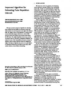
To deal with this problem, one should be given a measure of the error at the estimated values of the Doppler. As shown in Figure 3.2.3, the Clustering algorithm calculates the error, denoted by C ( j ) , between the estimates and the average of the estimates of Doppler that is the same as the calculation of variance. At the actual Doppler frequency, the variance by the PRFs should be the minimum. Without any noise, the C ( j ) should be zero at the actual Doppler frequency. The value of C ( j ) at the original Doppler will also be the same as the variance for the noise in the measurement and the maximum may be obtained by the Cramer-Rao bound. The average squared error C ( j ) for m consecutive Doppler is C( j ) =

1 j+m ∑ f oi − f m i = j +1

2

,

(3-2-28) where f = the average value of the m ordered Doppler, m = number of the PRF, f oi = tested frequency for i-th PRF and o times the folded one. Consider a Doppler frequency of 25.5kHz to illustrate how the algorithm works for the multiple PRF systems. If the three PRFs are PRF1 = 5kHz, PRF2 = 6kHz, PRF3 = 7kHz, then C ( j ) can be calculated and is shown in Figure 3.2.4. C ( j ) is minimized at the target frequency of 25.5kHz which is equal to the argument j = 63.

10

10

7

6

C(j)

10

8

10

10

5

4

0

10

20

30

40

50 j

60

70

80

90

Figure 3.2.4. The result of applying the clustering algorithm.

24

100

3.3 LEAST SQUARES METHOD The concept of spectral analysis to nonuniformly sampled data using Least squares was first proposed by Vanicek in 1970 [10]. Lomb (1975) developed this method and showed that a correlation exists between the height of the spectrum at any two frequencies which is equal to the mean height of the spectrum due to a sinusoidal signal of frequencies f 1 and f 2 [11]. These correlations reduce the distortion in the spectrum of a signal affected by noise which is an additional benefit to using unevenly spaced data [11]. Further studies have been done by Scargle (1982) in which he provided a simple estimate of the significance of the height of a peak in the power spectrum through the false alarm probability [19]. Feraz-Mello used non-orthogonality of the basis functions when the sampling is uneven and then applied the Gram-Schmidt orthogonalization procedure which is basically equivalent to a periodogram based method [21]. The periodogram approach to the evaluation of the spectrum form a set of nonuniformly sampled data provides a scan of a given frequency range. This is obtained by fitting sines and cosines functions in a Least squares fashion to the data and plotting the correlation of the data for each frequency. The Least square spectrum provides the best measure of the power contributed by the different frequencies to the overall variance of the data. Therefore this can be regarded as the natural extension of the Fourier methods to nonuniformly spaced data. The frequency increment can be determined with any precision and that is an additional benefit of using this method. Additional advantages can be derived from the uneven or random sampling which is absence of aliasing if the sampling were to be completely random [9, 13, 15]. It is known that in such situations the spectrum would be completely alias free [12]. Even though the periodogram analysis has many benefits, it also has some drawbacks. For example it cannot evaluate the spectrum for negative frequencies since it is a power spectrum of a real sequence. The estimated peak does not precisely correspond to the true magnitude of the signal. The error in the peak is mainly from the nonuniform spacing, which does not have the same source of error as in the FFT in which the error is primarily due to the finiteness of the sequence. A formulation that can resolve both positive and negative frequencies without loosing any of the benefits of the periodogram approach has been studied in this section. Additional properties of the Least squares approach have been investigated in section 3.3.2 to reduce the number of computations in a real time operation. 3.3.1 Formulation of the Least Squares Method Let a continuous complex signal x(t ) be sampled at time instants, t = t k , for k = 0, 1, 2,

…, N−1. We are interested in looking for a harmonic component of frequency ω , so that h(t ) = (a + ib) cos[ω (t − τ )] + (c + id ) sin[ω (t − τ )]

(3-3-1)

where a, b, c, d and τ are real constants. The delay parameter τ enables one to select any arbitrary location of the origin in the time axis. To estimate a, b, c and d the following mean square difference is minimized,

25

N −1

F = ∑ x(t k ) − (a + ib) cos[ω (t k − τ )] − (c + id ) sin[ω (t k − τ )]

2

(3-3-2)

k =0

with respect to the unknowns. Taking derivative of F with respect to the unknowns a, b, c and d will produce the normal equations which are of the form dF =0 da

or equivalently N −1

N −1

∑ x (t k ) cos[ω (t k − τ )] + ∑ x(t k ) cos[ω (t k − τ )] k =0

k =0

N −1

N −1

k =0

k =0

= 2a ∑ cos 2 [ω (t k − τ )] + 2c ∑ cos[ω (t k − τ )] sin[ω (t k − τ )] ,

(3-3-3)

where x (t k ) is the complex conjugate of x(t k ) . Since τ is a free parameter, it is selected so as to simplify the normal equations; that is, N −1

∑ cos[ω (t k =0

Solving for τ will yield

k

− τ )]sin[ω (t k − τ )] = 0 .

N −1 ∑ sin(2ωtk ) k tan (2ωτ) = = 0 . N −1 ∑ cos(2ωtk ) k =0

(3-3-4)

(3-3-5)

Similarly for the parameters b, c and d, we enforce dF dF dF = = = 0. db dc dd

Use of (3-3-4) will yield the following equations N −1

∑ ix (t ) cos[ω (t k =0

k

N −1

∑ x (t )sin[ω (t k =0

k

k

k

N −1

N −1

k =0

k =0

− τ )] − ∑ ix(t k ) cos[ω (t k − τ )] = 2b∑ cos 2 [ω (t k − τ )] , N −1

N −1

k =0

k =0

− τ )] + ∑ x(t k ) sin[ω (t k − τ )] = 2c ∑ sin 2 [ω (t k − τ )] ,

26

(3-3-6)

(3-3-7)

N −1

N −1

N −1

k =0

k =0

k =0

∑ ix (t k )sin[ω (t k − τ )] − ∑ ix(t k )sin[ω (t k − τ )] = 2d ∑ sin 2 [ω (t k − τ )].

(3-3-8)

The resulting values are: N −1

∑ Re[x(t k )]cos[ω (t k − τ )]

a=

k =0

N −1

∑ cos [ω (t

− τ )]

2

k =0

k

N −1

c=

k

N −1

∑ sin [ω (t k =0

k

k

k =0

N −1

∑ cos [ω (t 2

k

k

− τ )]

,d=

∑ Im[x(t )]sin[ω (t k

k =0

N −1

∑ sin [ω (t 2

k =0

k

− τ )]

k

N −1

− τ )]

− τ )]

2

, b=

∑ Im[x(t )]cos[ω (t k =0

∑ Re[x(t )]sin[ω (t k =0

N −1

k

,

− τ )]

− τ )]

,

(3-3-9)

.

(3-3-10)

and N −1

a + ib =

∑ x(t ) cos[ω (t k =0 N −1

k

∑ cos [ω (t 2

k =0

k

k

N −1

− τ )]

, c + id =

− τ )]

∑ x(t )sin[ω (t k =0 N −1

k

∑ sin [ω (t 2

k =0

k

− τ )]

k

− τ )]

Substituting (3-3-10) into (3-3-1) will yield N −1

h(t ) =

∑ x(t ) cos[ω (t k =0 N −1

k

∑ cos [ω (t 2

k =0

k

k

− τ )]

− τ )]

N −1

cos[ω (t − τ )] +

∑ x(t )sin[ω (t k =0 N −1

k

∑ sin [ω (t 2

k =0

k

k

− τ )]

− τ )]

sin[ω (t − τ )]

(3-3-11)

The power in the harmonic component at frequency ω is given by N −1

P(ω ) = ∑ h(t k , ω )

2

= a + ib

2

k =0

N −1

∑ cos 2 [ω (t k − τ )] + c + id

2

k =0

2

N −1

∑ sin [ω (t 2

k =0

− τ )]

2

⎧ N −1 ( ) [ ( ⎫ ⎧ N −1 ( ) [ ( ⎫ ⎨ ∑ x t k sin ω t k − τ )]⎬ ⎨ ∑ x t k cos ω t k − τ )]⎬ ⎭ . ⎭ + ⎩ k =0 = ⎩ k =0N −1 N −1 ∑ cos 2 [ω (tk − τ )] ∑ sin 2 [ω (t k − τ )] k =0

k

(3-3-12)

k =0

Equation (3-3-12) is a complex version of the Lomb periodogram [11]. Observe that (3-312) yields the same value for ω and − ω since it is squared. Obviously, this expression is not suitable for negative frequencies. To obtain the phase component of the spectrum from the power representation (3-3-12), a frequency response E (ω ) of the following form is assumed:

27

[

N −1

]

[

N −1

]

E (ω ) = ∑ α cos ω (t k − τ ) + i ∑ β sin ω (t k − τ ) , k =0

(3-3-13)

k =0

where τ is a free parameter as defined in (3-3-1). The corresponding power spectrum can be written as P (ω ) = E (ω )

2

∑ α cos[ω (t

=

k =0

2

]

N −1

−τ )

k

∑ β sin [ω (t

]

N −1

+

k =0

−τ )

k

2

.

(3-3-14)

Matching (3-3-12) and (3-3-14) for all x(t k ) will give the unknown coefficients α and β , i.e.,

∑ x(t ) cos[ω (t

]

N −1

∑ α cos[ω (t N −1 k =0

k

]

−τ ) = ±

k

k =0

∑ cos [ω (t

k

−τ )

∑ x(t ) sin [ω (t

−τ )

k =0

N −1

∑ β sin [ω (t k =0

k

]

−τ ) = ±

k

k =0

∑ sin [ω (t N −1

2

k =0

Thus,

[

N −1

E (ω ) = ±

k

,

]

N −1

2

N −1

−τ )

k

k

]

]

−τ )

.

(3-3-15)

] ∑ x(t )sin [ω (t

∑ x(t k ) cos ω (t k − τ ) k =0

∑ cos [ω (t

]

N −1

±i

k

k

k =0

∑ sin [ω (t N −1

−τ )

2

k =0

N −1

2

k =0

k

k

]

−τ )

.

]

−τ )

(3-3-16)

There can be four possibilities of choosing a sign and the problem is how to choose the correct one. The expression for the correct frequency can easily be obtained from the analogy of the conventional Fourier transformation or by inserting the following test signal x (t k ) = e iω t and observing (3-3-16) at the frequency ω 1 and − ω 1 . The resulting expression takes positive signs for both the terms, i.e., 1 k

∑ x(t ) cos[ω (t N −1

E (ω ) =

k

k =0

∑ cos [ω (t N −1

2

k =0

k

k

] ∑ x(t N −1

−τ )

]

+i

−τ )

k =0

k

)sin [ω (t k − τ )]

∑ sin [ω (t N −1

2

k =0

The phase information can be obtained using this expression.

28

k

]

−τ )

.

(3-3-17)

To illustrate the significance of (3-3-12) and (3-3-17), consider a signal of the form f ( x k ) = e 2⋅2πtk i + 2e −3.5⋅2πtk i − 2.5e 4⋅2πtk i , where t k is a random number uniformly distributed between [0, 100] for k = 1, 2, … , 100. Observe that this is the same signal as in the section 3.1 except for the average sampling frequency is much higher than the previous one. Now (3-3-12) and (3-3-17) are used to estimate the spectrum of the nonuniformly sampled data and the result is shown in Figure 3.3.1. Average sampling frequency is 1 Hz which is much lower than the Nyquist sampling rate (4 Hz since this is a complex signal). Here, the sampling frequency corresponds to the highest vale of the signal and not twice the highest frequency as required for the conventional Nyquist sampling theorem to hold. As seen in Figure 3.3.1(b) the negative frequency component located at –3.5 Hz is now distinguishable through the use of Equation (3-3-17). This is not possible in Figure 3.3.1(a) which is the original formulation for the Lomb periodogram. Note that the absolute value has been taken and squared in Figure 3.3.1(b). (a) Lomb Periodogram using (3-3-12) 800 600 400 200 0 -5

-4

-3

-2

-1

0

1

2

3

4

5

3

4

5

(b) Modified one using (3-3-17) 1500

1000

500

0 -5

-4

-3

-2

-1 0 1 Frequency [Hz]

2

Figure 3.3.1 Comparison between the Lomb periodogram and the new modified scheme.

3.3.2 Hilbert Transform Relationship We can reduce the computation time in the evaluation of the spectrum time by using a Hilbert transform relationship between the real and the imaginary parts of (3-3-17), E (ω ) . This means that the time domain response of E (ω ) is causal and this is shown next. The Hilbert transformation can be obtained by performing two Fast Fourier transforms and one multiplication. Assume that the number of frequency steps is M, and then the operation count for the Hilbert transform will be 2MlogM+M. The operation count for the

29

evaluation of Equation (3-3-17) is 4(N+1)M where N is the number of time domain data samples. By utilizing the Hilbert transform relationship the real part of (3-3-17) can be obtained from the imaginary part, and vice versa with reasonable accuracy and the 2 log(M ) + 1 + (2 N + 2) approximately. If processing time will be reduced by a factor of 4N + 4 M and N are large numbers, a maximum of 50% of reduction in the computation time by utilizing the Hilbert transformation is obtained. Assume a causal time domain signal x(t ) which exists on [0, α ] where α is a finite number, then E (ω ) =

∑ x(t )cos(ω t ) ∑ x(t )sin(ω t ) k

k

k

k

+i

∑ cos2 (ω tk )

k

k

k

∑ sin 2 (ω tk )

.

(3-3-18)

k

Here, the term τ is ignored since α is assumed to be a large number compared to the period of the signal and it is assumed that x(t ) is a time invariant sequence. When the time step is small, we can replace the summation in (3-3-18) by an integration, i.e., α

E (ω ) =

α

∫ x(t ) cos(ω t ) dt

+i

0

α

∫ cos (ω t ) dt

∫ x(t )sin (ω t ) dt 0

α

∫ sin (ω t ) dt

2

.

(3-3-19)

2

0

0

Application of

α sin (2ωα ) sin (2ωα ) 2 ∫0 cos (ω t ) dt = 2 + 4ω , ∫0 sin (ω t ) dt = 2 − 4ω ,

α

α

α

2

will transform equation (3-3-19) to α

E (ω ) =

∫ x(t ) cos(ω t ) dt 0

E (ω ) ≈

+i

∫ x(t )sin (ω t ) dt 0

sin (2ωα ) − 2 4ω

α

.

(3-3-20)

sin (2ωα ) > 1 , then 2

sin (2ωα ) + 2 4ω

α

α

α

α ∫0

x(t ) cos(ω t ) dt + i

30

2

α

α

∫ x(t )sin (ω t ) dt . 0

(3-3-21)

Since x(t ) is causal, the real and imaginary part of E (ω ) will be related by the Hilbert transform relationship when ωα >> 1 . Figure 3.3.2 compares E1 (ω ) with the Hilbert

transform of E 2 (ω ) where E (ω ) = E1 (ω ) + iE 2 (ω ) and E1 (ω ) , E 2 (ω ) are real. Figure 3.3.2(a) corresponds to the case, when ωα is relatively a large number, and then the two results will coincide with each other. When ωα is small, Figure 3.3.2(b) shows that there are some differences between the two curves where ω is of a small value. To illustrate the applicability of this method we consider the same signal as in the previous example: f ( x k ) = e 2⋅2πtk i + 2e −3.5⋅2πtk i − 2.5e 4⋅2πtk i ; 0 < t k < α

and the Matlab function HILBERT is used to compute the Hilbert transform of E 2 (ω ) . Processing time to obtain the estimator (3-3-17) can be measured by changing the number of frequency steps and the number of time domain data samples. The result is shown in Figure 3.3.3. By utilizing the Hilbert transformation, the processing time has been reduced by 46%. (a) When α is large (α = 2) 40 20 0 E1 Hilbert transformed from E2

-20 -40 -5

-4

-3

-2

-1

0

1

2

3

4

5

3

4

5

(a) When α is small (α = 0.5) 40 20 0 -20 -40 -5

E1 Hilbert transformed from E2 -4

-3

-2

-1 0 1 Frequency [Hz]

2

Figure 3.3.2 E1 (ω ) and Hilbert transform of E 2 (ω ) for different value of coincide with each other as shown in (a).

ωα .

If

ωα >>1 results

3.3.3 Estimation of the amplitude As seen in Figure 3.3.1, none of the Lomb periodogram methods or the modified ones provide the exact amplitude of the signal. The error obviously comes from the uneven spacing and the aliasing between the different frequencies.

31

Since the estimates of the frequencies giving rise to the peaks are not much different than the actual ones, we can estimate their amplitudes from these frequencies by using a Least square method. If the signal is a sum of exponentials, then L

x(t k ) = ∑ Al e iω l t k ; k = 1, 2, ..., N,

(3-3-22)

l =1

where ω l x(t k ) L and Al

= = = =

frequencies which give highest peaks, given data with respect to unevenly spaced point t k , number of frequency components, unknown magnitudes.

CPU time 1

(a) CPU time reduces by 46% when using the Hilbert transform

Number of time domain data = 100

0.8

Equation (3-3-17)

0.6 0.4

Hilbert transform

0.2 0 100

CPU time 0.4

200

300

400 500 600 700 Number of frequency steps

800

900

1000

900

1000

(b) CPU time reduces by 47% when using the Hilbert transform

0.35 Number of frequency steps = 100 0.3 Equation (3-3-17) 0.25 0.2 Hilbert transform 0.15 0.1 0.05 100

200

300

400 500 600 700 Number of time domain data

800

Figure 3.3.3 Processing time is reduced by using the Hilbert transform relationship.

By rewriting (3-3-22) as

32

⎡ x (t1 ) ⎤ ⎡ eiω1t1 ⎢ x (t ) ⎥ ⎢ iω1t2 ⎢ 2 ⎥ ⎢e ⎢ M ⎥=⎢ M ⎥ ⎢ ⎢ ⎥ ⎢ ⎢ ⎢⎣ x (t N )⎥⎦ ⎢eiω1t N ⎣

eiω 2t1

eiω 2 t2

M eiω 2t N

L eiω L t1 ⎤ ⎥ L eiω L t2 ⎥ O M ⎥ ⎥ ⎥ L eiω L t N ⎥⎦

⎡ A1 ⎤ ⎢A ⎥ ⎢ 2⎥ ⎢ M ⎥ ⎢ ⎥ ⎣ AL ⎦

(3-3-23)

and using the pseudo inverse, a vector A containing all the amplitudes can be obtained from the unevenly sampled points of the signal x(t k ) corresponding to the estimated frequency ω k as, A = (B * B ) B * f −1

⎡ e iω1t1 ⎢ iω1t2 ⎢e where B = ⎢ M ⎢ ⎢ ⎢e iω1t N ⎣

e iω 2t1 e iω 2 t 2 M e iω 2 t N

(3-3-24)

L e iω Lt1 ⎤ ⎥ L e iω Lt2 ⎥ and B * is a conjugate transpose of B. O M ⎥ ⎥ ⎥ iω L t N ⎥ L e ⎦ N ×L

The same signal as described by the first example has been used to verify (3-3-24) and the result is shown in Figure 3.3.4. The three signal components with unit amplitudes can be obtained precisely by utilizing (3-3-24) while the amplitudes obtained from using (3-2-17) have some differences when compared with the true value. Magnitude

1.2

1

0.8

0.6 Original Equation (3-3-17) Equation (3-3-24)

0.4

0.2

0 -200

-150

-100

-50

0 50 100 Frequency [rad]

150

200

250

300

Figure 3.3.4 Result of Equation (3-3-19). Since the periodogram does not give accurate values of the amplitudes, (3-3-19) can be used.

33

3.3.4 Summary Unevenly spaced spectrum using the Least squares method has been studied in this chapter. The well-known Lomb periodogram approach has many benefits but it cannot discriminate between positive and negative frequencies. Using a modified scheme, positive and negative frequencies can be discerned without losing any of the benefits of the Lomb periodogram. The method to estimate the magnitude of the signal using the periodogram approach has also been described. One of the properties of the periodogram approach is that a Hilbert transform pair relates the real and imaginary parts of the coefficients. By utilizing this property, the computation time for the spectrum can be reduced by half.

3.4 MULTI-RESOLUTION ANALYSIS In an effort to reconstruct a band-limited signal from an unevenly sampled signal using multirate filter banks, a multi-resolution approach has been taken by Vaidyanathan [25, 26 and 27]. It is possible to reconstruct a band-limited sequence from a data sequence followed by decimation. Since the spacing of the multiple PRF is not uniform and is not totally random, it can be characterized by an unevenly decimated version of the signal. In that case, one can utilize quadrature mirror filters (QMF) to get the original signal. Two preliminary conditions should be satisfied when using this approach to reconstruct a signal from an unevenly sampled data. First, the signal should be band-limited. In real life, there cannot be a band-limited sequence since our sample length in time is finite. If numerous data points are obtained or the signal spectrum is concentrated in a certain region, then one can consider the signal to be approximately band-limited for all practical purposes. Second, the sampling frequency cannot be totally random but it should have a common interval so that each sample in the multiple PRF signal is an integer multiple of the common interval. Since multiple PRF system satisfies the second condition, the main contribution to the error would be the finiteness of the data samples and the accuracy in the design of the filters. This method illustrates the correlation between sampling rate and the bandwidth. If the bandwidth becomes large, the number of samples should increase within a given period of the signal so as not to loose any information. Conversely, if the number of data samples becomes small, like missing data or due to decimation of the data, the bandwidth should decrease proportionally. In an ideal case, the QMF analysis can recover the unknown samples in between the missing data exactly. A two PRF case has been presented in this section and this can be extended to the multiple PRF case. 3.4.1 Two PRFs Case (20kHz and 30kHz) It is known that if a sequence is band-limited and the average sampling rate satisfies the Nyquist sampling criterion, then the sequence can fully be recovered regardless of the sampling rate whether it be uniform or not. Assume that we have M uniform samples in a period, then the maximum angular frequency content of the signal would be ω ≤ π . If

we have a decimated sequence which has N randomly chosen samples out of M uniform

34

samples, then the bandwidth of the sequence should be reduced to ω ≤ π

N for a M

complete recovery of the signal without aliasing. Figure 3.4.1 provides an example of the data sampled by two PRFs, 20kHz and 30kHz. Since the greatest common divisor of those two frequencies are 60kHz, the sequence is repeated every 6 intervals (every 4th sample). We want to recover the missing 2 samples 4 occurring at time step 1 and 5 out of 6 samples from a band limited sequence of ω ≤ π . 6 Perfect reconstruction can be achieved by a QMF system shown in Figure 3.4.2 if we can derive a set of filter banks which can carry out a perfect reconstruction of X ( z ) . Hence, the missing samples can be recovered. The intermediate step labeled U i s in Figure 3.4.2 is the unevenly sampled sequence. One can estimate the output Xˆ ( z ) using Equations (3-41) and (3-4-2). The output z transformation of the M-fold decimator (up sampler) Y ( z ) is [25]: Y ( z) =

1 M

M −1

∑ X ⎛⎜⎝ z

1

− j 2 πk M

M

e

k =0

⎞⎟ . ⎠

(3-4-1)

1

= 20 kHz

= 30 kHz

0

-1 0

4

2

6

10

8

12

14

16

18

20

Figure 3.4.1 Data generated by sampling a signal using 2 PRFs (20kHz and 30kHz). X (z )

↓6

U1

↑6

H1

↑6

H2

↑6

H3

↑6

H4

V1

z −2 ↓6

U2

V2

z −1 ↓6

U3

V3

z −1 ↓6

U4

V4

Xˆ ( z ) = z − k X ( z )

Figure 3.4.2. Block diagram for the reconstruction of the band-limited signal when sampled by the 2 PRFs (20kHz and 30kHz).

35

The output Z transform of the L-fold expander (down sampler) Y(z) is given by [25]: Y ( z) = X ( z L ) . − j 2π

We define W = e equation (3-4-1), as

M

=e

− jπ

3

(3-4-2)

and the U i in the Figure 3.4.2 would be obtained using

U 1 ( z) =

(

)

1 1 5 X z 6W k , ∑ 6 k =0

(

) X (z

1

1 5 16 k ∑z W 6 k =0

(

) X (z

1

(

) X (z

1

U 2 ( z) =

1 5 16 k ∑z W 6 k =0

U 3 ( z) = U 4 ( z) =

1 5 16 k ∑z W 6 k =0

−2

−3

−4

6

6

)

Wk ,

(3-4-3)

)

Wk ,

6

)

Wk .

By using (3-4-2), the Vs are given by V1 (z ) =

( )

1 5 k ∑ X zW H1 , 6 k =0

( ) ( )

V2 (z ) =

1 5 k −2 X zW k H 2 , ∑ zW 6 k =0

V3 (z ) =

1 5 k −3 X zW k H 3 , ∑ zW 6 k =0

V4 (z ) =

1 5 k −4 X zW k H 4 . ∑ zW 6 k =0

(3-4-4)

( ) ( )

( ) ( )

The output Xˆ ( z ) will be the sum of all the Vi ’s and this should be a purely delayed version of the original sequence if it were to be a perfect reconstruction of our signal. Thus, Xˆ ( z ) = V1 ( z ) + V2 ( z ) + V3 ( z ) + V4 ( z )

36

[

(

)

⎧ X ( z ) + X ( zW ) + X zW 2 + X ⎪ −2 −4 1 ⎪+ X ( z ) + W X ( zW ) + W X = ⎨ 6 ⎪+ X ( z ) + W −3 X ( zW ) + W −6 X ⎪+ X ( z ) + W − 4 X ( zW ) + W −8 X ⎩

[ [ [

(zW (zW (zW (zW

3

) + X (zW ) + X (zW )]H ) + W X (zW ) + W X (zW ) + W X (zW )]z H ) + W X (zW ) + W X (zW ) + W X (zW )]z H ) + W X (zW ) + W X (zW ) + W X (zW )]z H 4

5

1

2 2 2

−6

3

−8

−9

3

−12

−12

3

−10

4

4

−16

4

= z − k X ( z) ,

−15

− 20

−2

5

−3

5

5

−4

(3-4-5)

where k is any constant. The aliased terms, X ( zW ) , X ( zW 2 ) , X ( zW 3 ) , X ( zW 4 ) and

X ( zW 5 ) , should be zero for perfect reconstruction and the output signal term should be a delayed version of the original signal. Matching term by term in each of the two expressions will yield

[

]

1 X ( z ) H 1 + z − 2 H 2 + z −3 H 3 + z − 4 H 4 = z − k X ( z ) , 6

(3-4-6-a)

[

]

(3-4-6-b)

[

]

(3-4-6-c)

[

]

(3-4-6-d)

[

]

(3-4-6-e)

[

]

(3-4-6-f)

1 X ( zW ) H 1 + W − 2 z − 2 H 2 + W −3 z −3 H 3 + W − 4 z − 4 H 4 = 0 , 6 1 X (zW 2 ) H 1 + W −4 z − 2 H 2 + W −6 z −3 H 3 + W −8 z − 4 H 4 = 0 , 6 1 X (zW 3 ) H 1 + W −6 z − 2 H 2 + W −9 z −3 H 3 + W −12 z − 4 H 4 = 0 , 6 1 X (zW 4 ) H 1 + W −8 z − 2 H 2 + W −12 z −3 H 3 + W −16 z − 4 H 4 = 0 , 6 1 X (zW 5 ) H 1 + W −10 z −2 H 2 + W −15 z −3 H 3 + W − 20 z − 4 H 4 = 0 . 6

We have 4 unknowns, H 1 , H 2 , H 3 and H 4 , and 6 equations which cannot be solved

simultaneously in general. In our case, the shifted terms X ( zW ) , X ( zW 2 ) , X ( zW 3 ) ,

X ( zW 4 ) and X ( zW 5 ) exist only in limited regions in the frequency domain and we can make those equations satisfy the constraints in each region. Figure 3.4.3 shows the shifted versions of the sequence X ( z) . In region 1 of Figure 3.4.3, Equation (3-4-6-a), (3-4-6-b),

(3-4-6-c) and (3-4-6-d) need to be satisfied since X ( zW 4 ) and X ( zW 5 ) are zeros and it satisfies all 6 equations in region 1. Solving the equations will give the filter characteristics in region 1. The filters, H 1 , z −2 H 2 , z −3 H 3 and z −4 H 4 , should be constant numbers for each frequency region since W is a constant. In region 2, Equation (3-4-6-a),

37

⎫ ⎪ 2 ⎪ ⎬ 3 ⎪ ⎪ 4⎭

(3-4-6-b), (3-4-6-c) and (3-4-6-f) need to be satisfied since X ( zW 3 ) and X ( zW 4 ) are zero and it satisfies all the six equations. Solving the equations will give the filters characteristics in the region 2. In region 3, Equation (3-4-6-a), (3-4-6-b), (3-4-6-e) and (34-6-f) need to be satisfied. X ( zW 2 ) and X ( zW 3 ) is zero which makes it possible to satisfy all the six equations, simultaneously. Solving the equations will give the filter characteristics in the region 3. In region 4, Equation (3-4-6-a), (3-4-6-d), (3-4-6-e) and (34-6-f) need to be satisfied since X ( zW ) and X ( zW 2 ) are zero and this satisfies all the 6 equations. Solving all these equations will give the filter characteristics in the region 4. Once the filter coefficients for each region are calculated, they should be combined to make a set of filters. Note that each filter from the equation yields H 1 , z −2 H 2 , z −3 H 3 and z −4 H 4 and the delay should be taken out from them when realizing the filters. The results of those filters are shown in Figure 3.4.4.

(a) The spectrum of a signal 1.2 1 0.8

÷ x(z)

0.6 0.4 0.2 0 -3

-2

-1

0

1

2

3

(b) Shifted versions of the spectrum 3 1 ÷ X(zW )

÷X(zW 4 )

÷X(zW 5)

÷X(z)

÷X(zW)

X(zW 4)÷ ÷ X(zW )

÷ X(zW 2 )

3

0.5

0

÷X(zW 2)

÷ Region 4 ÷ ÷ Region 3 ÷ ÷ Region 2 ÷ ÷ Region 1 ÷ -3

-2

-1

0 Frequency [rad]

1

2

Figure 3.4.3 Spectrum of a sampled signal and its shifted versions.

38

3

Real part of H1

Imaginary part of H1

2.5

2

2

1

1.5

0

1 -1

0.5 0

-2 -2

0 2 Real part of z -2H2

-2 0 2 Imaginary part of z -2H2

2.5

2

2

1

1.5 0 1 -1

0.5 0

-2 -2

0

2

-2

Real part of z -3H3

0

2

Imaginary part of z -3H3 2

3 1 2

0

1 0

-1 -2

-2

0 2 -4 Real part of z H4

2.5

2

2

1

-2 0 2 -4 Imaginary part of z H4

1.5 0

1

-1

0.5 0

-2 -2

0

2

-2

0

2

Figure 3.4.4 Filters to generate a perfect reconstruction of the signal for the system of Figure 3.4.2.

A numerical example outlined in Figure 3.4.2 utilizing the system of filters as described in Figure 3.4.4 is used to illustrate how this method performs. The original signal is described by f ( x k ) = e 2⋅2πxk i + 2e −3.5⋅2πxk i − 2.5e 4⋅2πxk i ; for k = 1, 2, …, 168.

(3-4-7)

The signal is sampled at 5.5556Hz and 8.3333Hz (equivalent sampling at 20kHz and 30kHz with time scaling) simultaneously as shown in Figure 3.4.1 and it is equivalent to sampling the signal at 16.6667 (60kHz) and then unevenly decimating it. Note that the maximum frequency in the signal is 4Hz which is less than half the equivalent sampling

39

frequency 5.5556Hz (= N M ⋅ 16.6667/2). The frequency domain result is given in Figure 3.4.5. Observe that the original signal is not strictly band-limited due to the finite number of data samples but the transformed one is band-limited. Figure 3.4.6 produces the resulting time domain sequence. 3.4.2 Multiple PRF Case The same procedure as described for the 2 PRF case can be applied to the multiple PRF case. Define M as the total number of time steps in one period where decimation repeatedly occurs. If the PRFs are relatively prime numbers of each other, the time step M will be given by the least common multiplier (l.c.m) of the PRFs. For example, the sampled data for the 3 PRFs 3Hz, 4Hz and 5Hz which are relatively prime numbers is repeated every 60 time steps as illustrated in Figure 3.4.7. If the PRFs are not relative prime numbers, then M should be divided by the greatest common divisor (g.c.d) of the PRFs. Sampling the data by PRFs of 3Hz, 4Hz and 5Hz is same as sampling the data at 30kHz, 40kHz and 50kHz except that the scale factor and M can be recalculated by dividing the PRFs with their g.c.d, i.e.,

M =

l.c.m(PRF1 , PRF2 L) . g .c.d (PRF1 , PRF2 L)

(3-4-7)

(a) Spectrum of the original sequence 400 300 200 100 0

-3

-2

-1

0

1

2

3

2

3

(b) Spectrum of the estimated sequence 400 300 200 100 0

-3

-2

-1

0 Frequency [rad]

1

Figure 3.4.5 Spectrum (magnitude) for the data of Figure 3.4.2 when using the QMF filters as shown in Figure 3.4.4.

40

(a) Original sequence 6 4 2 0

0

0.2

0.4

0.6

0.8

1

1.2

1.4

1.6

1.8

(b) Estimated sequence 6 4 2 0

0.4

0.6

0.8

1

1.2 1.4 Time

1.6

1.8

2

Figure 3.4.6 Time domain data for the example of Figure 3.4.2 when using the QMF filters as shown in Figure 3.4.4.

The number of known samples in one period adds up to the PRFs reduced by 1 if they are relative prime numbers. If they are not relative prime numbers, it can simply be divided by their g.c.d. as before. Define N as the number of known samples in the M time intervals, where

N=

∑ PRF

i

i

g.c.d (PRF1 , PRF2 L)

−1.

(3-4-8)

For the 30kHz, 40kHz and 50kHz case we will have 11 known samples in one period. We have 49 (= 60 − 11) unknown samples in one period in this case (represented by the dots in Figure 3.4.7). The ratio of the number of unknown samples to the known samples determines the maximum bandwidth of the signal with respect to the Nyquist rate. The real data sampled by the exact Nyquist frequency or at a higher frequency can have a maximum bandwidth of 2 times the Nyquist frequency for an exact reconstruction. A more sparsely sampled data than the Nyquist rate should have less bandwidth for an exact reconstruction. The maximum bandwidth allowed for the signal would be

ω ≤π

N . M

Obviously, the bandwidth if sampled by the Nyquist rate is ω ≤ π .

41

(3-4-9)

2

= 30kHz

= 40kHz

20

30

= 50kHz

1

0 0

10

40

50

60

Figure 3.4.7 Sampled data generated by the three PRFs.

Even though the signal is band-limited by Equation (3-4-9), the effective sampling frequency increases to the l.c.m of those three PRFs of 3, 4 and 5Hz which is 60Hz. The actual maximum resolvable Doppler frequency also increases. The number of filters that should be designed is the same as the number of known samples (N) as in the Figure 3.4.2. The spectra should be divided into M regions to 2π calculate each of the filter coefficients. The bandwidth for each region will be (for the M 2π ) and this can be a limitation for realizing a filter when M 20kHz and 30kHz case it is 6 is a large number with a finite number of sampling points. For the 3 PRF case, 30kHz, 40kHz and 50kHz, the total number of filters in Figure 3.4.2 will be 11 and the maximum 11 bandwidth of the signal would be ω ≤ π when the sampling rate is 600kHz (= l.c.m of 60 30kHz, 40kHz and 50kHz). This is equivalent to sampling the data at 110kHz (= 600×11/60) since there is both a reduction of the bandwidth and an increase of the sampling frequency. That is, the maximum resolvable Doppler frequency is increased by 2.75 (=110/40) times over the single PRF case of 40kHz. In this case the maximum resolvable range increases by 4 (=40/10) times that of the single PRF system of 40kHz. 2π 2π The bandwidth of each region for the QMF is = . M 60 3.4.3 Optimum Value of M and N in Radar Application This method has two practical limitations as indicated earlier which causes errors in the estimation. First, assume that the signal is a band limited sequence. In a real situation obtaining a band limited sequence through a finite number of samples is not possible. In radar applications, typically the maximum number of samples does not exceed a few hundred points. In which case, our reconstruction of spatial domain data will have inherent errors. This is shown in the previous example of Figure 3.4.5. The other limitation is the bandwidth of each region. Each of the filters to be implemented in each of the region has an M band filter characteristic [25] and the bandwidth becomes too small if M becomes large. For the 3 PRF case of 30kHz, 40kHz and 50kHz, we need a filter which has a 2π 2π bandwidth of = . This type of filter is difficult to implement since there are only a M 60 few hundred sample points.

42

The range increment by using a multiple PRF system is proportional to 1/PRF and it is given by PRF2 , (3-4-10) IR = g.c.d (PRF1 , PRF2 L) where IR is the increase of the scale factor in terms of the range and PRF2 is the PRF used for comparison with that of a single PRF system. The maximum resolvable range for the 30kHz, 40kHz and 50kHz PRF cases will be 4 (= 40/10) times that of the single PRF case corresponding to 40kHz. The increase in the range of the Doppler by using a multiple PRF system can be seen from the following equation ID = Bandwidth × f s =

N l.c.m(PRF1 , PRF2 L) , M PRF2

(3-4-11)

where ID is the increase in the range of the Doppler, Bandwidth is the ratio of the maximum signal bandwidth divided by two times the Nyquist rate and f s is the equivalent sampling frequency of the multiple PRF system. The maximum resolvable Doppler for the 30kHz, 40kHz and 50kHz PRF case is 11/4 times that of the one PRF case of 40kHz. Since there is a trade-off between maximum Doppler and maximum range [1, 2], we want to maximize the incremental product of the of Doppler and the range, that is,

ID × IR =

=

PRForig N LCM (PRF1 , PRF2 L) × M PRForig GCD(PRF1 , PRF2 L) N

LCM ( PRF1 , PRF2 L)

GCD( PRF1 , PRF2 L)

LCM ( PRF1 , PRF2 L) PRForig

= N.

×

PRForig

GCD( PRF1 , PRF2 L)

(3-4-12)

We can maximize N with respect to M. From this result one can choose N = M−1 since N should always be less than M. For the case of M = 16 and N = 15, the results are shown in Figure 3.4.8 and 3.4.9 when applied to the same signal as in the previous example (3-4-7). Note that Equation (3-4-10) is true for the general multiple PRF system and Equation (34-11) is applicable only when using the QMF filters. Therefore the result of (3-4-12) may be different if other reconstruction techniques are used.

43

(a) Spectrum of the original sequence 400 300 200 100 0

-3

-2

-1

0

1

2

3

2

3

(b) Spectrum of the estimated sequence 400 300 200 100 0

-3

-2

-1

0 Frequency [rad]

1

Figure 3.4.8 Frequency domain response for the optimized case (M = 16, N = 15).

(a) Original sequence 6 4 2 0

0

0.2

0.4

0.6

0.8

1

1.2

1.4

1.6

1.8

(b) Estimated sequence 6 4 2 0

1

1.2

1.4

1.6

1.8 Time

2

2.2

2.4

2.6

Figure 3.4.9 Result for the example (magnitude) in the time domain (M=16 and N=15).

3.5 Iterative Method

The application of iterative methods based on the Sandberg’s theorem [20] was first used for evaluating the spectrum of a nonuniformly sampled data by Willy [29]. Willy used pulses of finite width and conjectured that the interactive recovery procedure will

44

converge for the finite width sampling. Marvasti [30] tried to prove that the iterative method converges for random samples when the samples are chosen from a uniform or a Poisson distribution. Sandberg proved the convergence of this method [31]. It is shown that if the signal is band-limited and the average sampling rate satisfies the Nyquist sampling rate, then the signal can be recovered [12, 13] without aliasing. The method uses an iterative procedure that requires low pass filtering of the unequally spaced samples followed by resampling at the same points. Again, low pass filtering is applied to the signal to obtain a corrected signal. Repeated application of this process is shown to converge to the original signal. The proof of convergence is given in Appendix C. By its nature, the iterative method is more time consuming than the other methods since it requires a large number of iterations. Even though the convergence is guaranteed by this method, the number of iterations can be very large to reach a certain error criteria. Some effort has been done by Park [24] to increase the rate of convergence by minimizing the energy term, but in their approach one needs to know the values for the error terms that is usually not known. Usually a smaller spacing between samples provides a faster convergence of the sequence. Starting with the Sandberg theorem, “On the properties of some systems that distort signals“ [31] Sandberg extended Beurling’s theory of recovery of distorted band-limited signals in a Hilbert space. He showed that signal recovery can be extended to the case in which a known square integrable noise is added to the input signal and the result applied to a time varying device which may be non-linear. Sandberg’s theorem can be stated as: Let P and Q be the mapping of κ into H (Hilbert space) such that for all f , g ∈κ Re(Qf − Qg , f − g ) ≥ k1 f − g , 2

PQf − PGg

2

2

≤ k2 f − g ,

(3-5-1) (3-5-2)

where k 1 and k 2 are positive constants. Then for each h ∈ κ, the equation h = PQf possesses a unique solution

( PQ) given by

( PQ)

−1

−1

h ∈κ ,

(3-5-3)

h = lim f n ,

(3-5-4)

n →∞

where f n +1 =

k1 (h − PQf n ) + f n , k2

(3-5-5)

and f 0 is an arbitrary element of κ. Furthermore, for all h1 , h2 ∈ κ

(PQ )−1 h1 − (PQ )−1 h2

45

≤

1 k1

h1 − h2 .

(3-5-6)

The proof is given in Appendix C. The uniqueness of the solution for h = PQz is also given in Appendix D. Applying theorem (3-5-6) to the unequally spaced signal, and letting P = band-limiting operator (Low pass filter), Q = ideal nonuniform sampling operator the same as in the given nonuniformly spaced samples, will transform the expressions in (3-5-4) and (3-5-6) as lim x k ( t ) = x( t ) ,

(3-5-7)

x k +1 ( t ) = λPQx( t ) + ( P − λPQ) x k ( t ) ,

(3-5-8)

k →∞

where x( t ) is the band-limited signal and λ is a constant. The constraint between the coefficient λ and data spacing t i are given in Appendix F and is given by 0 f max As mentioned in the previous sections, the polynomial interpolation method, iterative method and orthogonal expansion method yield better estimation for the spectrum when the sampling frequency becomes much higher than the Nyquist frequency. These approaches usually provide a meaningful result when the average sampling rate is at least 4 times that of the maximum frequency of the signal. In the numerical example, the sampling frequency has been chosen to be 4 times that of the maximum signal frequency. For the first example, we examine a single frequency signal of magnitude 10. Example 1: Single frequency f s = 4 f max The average sampling rate is 14Hz and the signal frequency is 3.5Hz. The non-uniformly spaced samples repeat every 14th sample and a total of 100 sampling points are taken so that f ( x k ) = 10 e 2πi⋅3.5 xk

with k = 1, 2, …, N. N = number of samples = 100.

The nonuniformly sampled time domain signal and the DFT of the original signal are shown in Figure 3.8.1(a) and (b). The frequency response has a peak at the signal frequency component, which is the 25th cell out of 100 cells. All the eight methods have been simulated and the results are given in Table 3.8.1. The error in the time domain has been computed by using the normalized average of the differences. The estimate of the signal is fˆ ( x k ) and the error in the approximation of the function is defined by N

∑

Error1 =

f ( x k ) − ˆf ( xk )

1 k =1 N max ⎛⎜ ⎝

f ( x k ) ⎞⎟ ⎠

.

(3-8-1)

The estimate of the error in the frequency domain is given in Table 3.8.1. It is computed by taking the differences between the maximum of the computed frequency response and the signal frequency indicated in the last column of Table 8.3.1 and is expressed by

Error 2 =

f − fˆ , f

(3-8-2)

where f is the target frequency and fˆ is the estimated frequency. fˆ is the frequency at which the maximum value of the frequency response is obtained. Note that the frequency domain error term is the difference between the computed spectrum of the time domain data and the actual frequency response. For the method

60

based on the CR theorem, we took 53 and 48 sample points for each sampling frequency. Observe that the peaks in the spectrum occurred at the 23rd and 24th cell since the sampling frequency of 8Hz and 7Hz will yield the cell number 23 ( ≈ 3.5 ⋅ 53 / 8 ) and 24 ( ≈ 3.5 ⋅ 48 / 7 ) for a target frequency of 3.5. Even though the time domain estimation is not very good, acceptable estimates for the target Doppler can be obtained for all the methods. In this example, all the methods provided acceptable estimates for the spectrum.

(a) Time domain sgnal 10

Real Imaginary

5 0 -5 -10 0

0.1

0.2

10

20

0.3

0.4

0.5 0.6 0.7 0.8 Time (b) FFT of the original signal(abs part)

0.9

1

1200 1000 800 600 400 200 0

0

30

40 50 60 70 Frequency cell number

80

90

Figure 3.8.1 Sample signal for Example 1

Table 3.8.1 Summary of the results for Example 1. f s = 4 f max with single frequency.

Methods Lagrange polynomial Cauchy’s method CR theorem Least squares method QMF method Iterative method Orthogonal polynomial approach Analog frequency approach

Error1 (time domain)

Error2 (frequency domain)

Number of data

Target cell number

0.3077 0.9267 0.2135 0.3294 2.6992E-4 -

0.0000 0.0000 0.0000 0.0000 0.0000 0.0000 0.0000 0.0000

44 44 48, 53 100 100 100 100 100

11 11 24, 23 25 25 25 25 25

Example 2: A Single frequency with noise The same signal as in Example 1 has been considered and additive white Gaussian noise (AWGN) has been added. The model for the noise signal is described by

61

Noise =

Pnoise

2

[N (0,1) + iN (0,1)] ,

(3-8-3)

where Pnoise is the noise power and N(0,1) follows a normal distribution with unit variance and zero mean. The signal model is defined by f ( x k ) = 10 e 2πi⋅3.5 xk + Noise .

Table 3.8.2 presents the probability of detection for each method as a function of the power associated with the noise process. We assume that a target has been detected when the computed spectrum has a peak which corresponds to the appropriate cell number for the target. Total number of trials for each method used to compute the probability of detection is 100. With an increase in SNR, the probability of detection increases as expected. Table 3.8.2 Result of Example 2.

f s = 4 f max with a single frequency and additive AWGN Probability of detection

Methods

Lagrange polynomial Cauchy’s method CR theorem Least squares method QMF method Iterative method Orthogonal polynomial approach Analog frequency approach

SNR [dB] 0 0.97 0.18 1.00 1.00 1.00 1.00 0.00 1.00

5 10 15 20 25 1.00 1.00 1.00 1.00 1.00 0.27 0.58 0.70 0.99 1.00 1.00 1.00 1.00 1.00 1.00 1.00 1.00 1.00 1.00 1.00 1.00 1.00 1.00 1.00 1.00 1.00 1.00 1.00 1.00 1.00 0.00 0.00 0.00 0.00 0.00 1.00 1.00 1.00 1.00 1.00

Number of data

Target cell number

44 44 48, 53 100 100 100 100 100

11 11 24, 23 25 25 25 25 25

Example 3: Multiple frequency signals and f s = 4 f max

In this example, the signal has 5 frequency components f ( x k ) = 10 e 2πi⋅0.35 xk + 8e 2πi⋅1.05 xk + 9e 2πi⋅1.4 xk + 2e 2πi⋅2.8 xk + 6e 2πi⋅3.5 xk

We assumed that the last component, 6e 2πi⋅3.5 xk , is the signal of interest (SOI) and the other components are interference. The frequency scanning is performed from 2Hz to 15Hz (equivalent from 14th to 100th cell in the frequency domain response) since the major interfering signals are located below 2Hz. The time domain signal and the corresponding frequency domain response are shown in Figure 3.8.2. Table 3.8.3 is the result of the simulations. The CR theorem approach has been deleted from the Table since it can only deal with a signal having a single frequency component. The highest degree of polynomial for the Cauchy’s method and for the Lagrange polynomial technique has been a bit higher

62

than in Example 1 since for Example 2 the signal has a stronger low frequency component than in Example 1. Example 4: Multiple frequency signal with noise For this example, the signal has five frequency components and is given by f ( x k ) = 10 e 2πi⋅0.35 xk + 8e 2πi⋅1.05 xk + 9e 2πi⋅1.4 xk + 2e 2πi⋅2.8 xk + 6e 2πi⋅3.5 xk + noise

The noise model is the same as in (3-8-3) and the SOI is the same as in Example 3. The results are presented in Table 3.8.4 using 100 trials. Except for the Cauchy’s method, all the other methods provided acceptable results for different values of the SNR. Because Cauchy’s method provides a fit to the data through the use of rational polynomials, it cannot precisely fit the noisy data that changes rapidly with time.

(a) Time domain sgnal 40 Real Imaginary

20 0 -20 -40

0

0.1

0.2

0.3

10

20

30

1000

0.4

0.5 0.6 0.7 0.8 Time (b) FFT of the signal magnitude

0.9

1

90

100

800 600 400 200 0 0

40 50 60 70 Frequency cell number

80

Figure 3.8.2 Sample signal for Example 3

Table 3.8.3 Summary of the results for Example 3. f s = 4 f max with 5 signal components Methods Lagrange polynomial Cauchy’s method Least squares method QMF method Iterative method Orthogonal polynomial approach Analog frequency approach

Error1 (time domain) 0.0454 0.0755 0.0785 0.0626 7.1196E-5 -

Error2 (frequency domain) 0.0000 0.0000 0.0000 0.0000 0.0000 0.0000 0.0000

63

Number of data 44 44 100 100 100 100 100

Target cell number 11 11 25 25 25 25 25

Table 3.8.4 Summary of results for Example 4. f s = 4 f max with 5 signal components and AWGN Probability of detection Methods

Lagrange polynomial Cauchy’s method Least squares method QMF method Iterative method Orthogonal polynomial approach Analog frequency approach

SNR [dB] 0 0.97 0.62 1.00 1.00 1.00 0.00 1.00

5 1.00 0.75 1.00 1.00 1.00 0.00 1.00

10 1.00 0.83 1.00 1.00 1.00 0.00 1.00

15 1.00 0.90 1.00 1.00 1.00 0.00 1.00

20 25 1.00 1.00 0.80 0.88 1.00 1.00 1.00 1.00 1.00 1.00 0.00 0.00 1.00 1.00

Number of data

Target cell number

44 44 100 100 100 100 100

11 11 25 25 25 25 25

In summary, when the sampling frequency is high compared to the highest frequency content of the signal, most of the methods presented in this report can be applied to estimate the spectrum of a nonuniformly sampled data sequence. But this case is of little use to the radar community since the maximum resolvable Doppler frequency is not very large as seen from (2-10). In the next case we will increase the signal frequencies (or decrease the average sampling rate) and will observe which approach has a better performance. 3.8.2 Case 2: f s = 2 f max When the sampling frequency equals twice the value of the maximum signal frequency, all polynomial methods approximating the time domain samples cannot be used since they need smaller sampling periods. Moreover, the results of the QMF method is only valid for the case when the average sampling rate is higher than the Nyquist sampling rate and its results will degrade in accuracy if it is less than or equal to the Nyquist sampling rate. Only three methods, the Least squares method, the CR theorem method and the analog frequency approach can be used for this particular case. In this example, the other conditions are the same as in case 1 except for the value of the signal frequency.

Example 5:

The signal used in this case is given by f ( x k ) = 10 e 2πi⋅7 xk and the results are given in Table 3.8.5. All the three methods yield good results. (3-8-1) and (3-8-2) has been used to get the error estimate. Table 3.8.5 Summary of the results for Example 5. f s = 2 f max with a single frequency Methods CR theorem Least squares method Analog frequency approach

Error1 (time domain) -

Error2 (frequency domain) 0.0000 0.0000 0.0000

64

Number of data 48, 53 100 100

Target cell number 0,46 50 50

Example 6: In this case, the signal is given by f ( x k ) = 10 e 2πi⋅7 xk + Noise and the noise is computed using (3-8-3). The results are given in Table 3.8.6. All three methods yield good results. Table 3.8.6 Summary of the results for Example 6. f s = 2 f max with a single frequency and AWGN Probability of detection Methods

CR theorem Least squares method Analog frequency approach

Number of data

Target cell number

48, 53 100 100

0, 46 50 50

SNR [dB] 0 1.00 1.00 1.00

5 1.00 1.00 1.00

10 1.00 1.00 1.00

15 1.00 1.00 1.00

20 25 1.00 1.00 1.00 1.00 1.00 1.00

Example 7: In this case the signal is of the form f ( x k ) = 10 e 2πi⋅0.7 xk + 8e 2πi⋅2.1 xk + 9e 2πi⋅2.8 xk + 2e 2πi⋅5.6 xk + 6e 2πi⋅7 xk

and the results are given in Table 3.8.7. The clustering algorithm was not used in this example when using the method based on the CR theorem since there are many frequency components, and therefore only the Least squares and the analog frequency approach can provide acceptable results. Table 3.8.7 Summary of results for Example 7. f s = 2 f max with five signal frequencies Methods Least squares method Analog frequency approach

Error1 (time domain) -

Error2 (frequency domain) 0.0000 0.0000

Number of data 100 100

Target cell number 50 50

Example 8: In this example, the signal plus noise is described by f ( x k ) = 10 e 2πi⋅0.7 xk + 8e 2πi⋅2.1 xk + 9e 2πi⋅2.8 xk + 2e 2πi⋅5.6 xk + 6e 2πi⋅7 xk + Noise

and the results are given in Table 3.8.8. The clustering algorithm was not used for the method based on the CR theorem as in this example there are many signals at different frequencies, and therefore only the Least squares method and the analog frequency approach yield good results. Example 9: Multiple signal frequencies with added noise and ground clutter

In this case, the signal has 5 frequency components along with additive Gaussian noise and ground clutter. f ( x k ) = 10 e 2πi⋅0.35 xk + 8e 2πi⋅1.05 xk + 9e 2πi⋅1.4 xk + 2e 2πi⋅2.8 xk + 6e 2πi⋅3.5 xk + noise + clutter.

65

Table 3.8.8 Summary of results for Example 8. f s = 2 f max with 5 signal frequencies and AWGN Probability of detection Methods

Number of data

Target cell number

100 100

50 50

SNR [dB] 0 5 10 15 20 25 0.97 1.00 1.00 1.00 1.00 1.00 1.00 1.00 1.00 1.00 1.00 1.00

Least squares method Analog frequency approach

The clutter model is given by

C (ω ) = 2000 e − ( 0.1ω )

2

(3-8-4)

and the corresponding frequency spectrum is shown in Figure 3.8.3. The noise model is the same as in (3-8-3) and the SOI is the same as in Example 3. The results are given in Table 3.8.5 by using 100 trials. The frequency is scanned from 2Hz to 7.5Hz (equivalent from 14th to 50th cell in the frequency domain response) since the major portion of the interference and the ground clutter is located below 2Hz. The simulation result is given in Table 3.8.9. (a) Ground clutter model in the frequency domain 2000 1500 1000 500

0

2000

10

20

30

40 50 60 70 Frequency (b) Received signal model in the frequency domain

80

← Interference

1500 1000

← Interference ← Interference

500

0

10

20

30

← Target 40 50 Frequency

60

70

80

Figure 3.8.3 Model for a ground clutter (evenly sampled data) Table 3.8.9 Summary of the results for Example 9. f s = 2 f max with 5 signal frequencies along with AWGN and ground clutter. Probability of detection

Methods

Least squares method Analog frequency approach

Number of data

Target cell number

100 100

50 50

SNR [dB] 0 5 10 15 20 25 1.00 1.00 1.00 1.00 1.00 1.00 1.00 1.00 1.00 1.00 1.00 1.00

66

In summary, when the sampling frequency is the same as the Nyquist sampling rate of a real signal, only three methods can be applied to evaluate the spectrum of a nonuniformly sampled data. In this case, it is possible to achieve a higher resolution as illustrated in (34-12). By using the three methods illustrated in this case, 10-20 times performance enhancement in terms of the maximum resolvable Doppler can easily be obtained. As mentioned earlier, the method based on the CR theorem cannot be used if multiple signals exist or if there is ground clutter. In the next example, we will further increase the number of signal frequencies and will observe which approach has a better performance. 3.8.3 Case 3: fs < fmax When the average sampling frequency is less than the maximum signal frequency, only the Least squares method and the clustering algorithm can be used. All other conditions remain the same as in case 1 and 2 except for the signal frequency. Example 10: For this example f s =

1 f max with a single signal frequency. 3

The data is given by f ( x k ) = 10 e 2πi⋅42 xk

and the results are given in Table 3.8.10. All the three methods yield good results. Here, (3-8-1) and (3-8-2) have been used to obtain an estimate of the error in the time and frequency domain. Note that the error in the clustering algorithm is due to the FFT of the data samples, which do not match exactly to the signal frequency. Table 3.8.10 Summary of results for Example 10. f s =

Methods CR theorem Least squares method

Error1 (time domain) -

1 f max with a single frequency 3

Error2 (frequency domain) 4.4881E-4 0.0000

Number of data 48, 53 100

Target cell number 0,13 300

Example 11: In this case, f ( x k ) = 10 e 2πi⋅42 xk + Noise and the noise are given by (3-8-3). The results are given in Table 3.8.11. Both methods yield good results. Table 3.8.11 Summary of the results for Example 11. f s =

1 f max with a single frequency and 3

AWGN Probability of detection

Methods

CR theorem Least squares method

Number of data

Target cell number

0 5 10 15 20 25 1.00 1.00 1.00 1.00 1.00 1.00

48+53

0,13

1.00 1.00 1.00 1.00 1.00 1.00

100

300

SNR [dB]

67

Example 12: In this case, the signal is of the form f ( x k ) = 10 e 2πi⋅4.2 xk + 8e 2πi⋅12.6 xk + 9e 2πi⋅16.8 xk + 2e 2πi⋅33.6 xk + 6e 2πi⋅42 xk

and only the Least squares method can be used. The results are given in Table 3.8.12. Table 3.8.12 Summary of the results for Example 12. f s =

Methods Least squares method

Error1 (time domain) -

1 f max with 5 signal frequencies. 3

Error2 (frequency domain) 0.0000

Number of data 100

Target cell number 300

Example 13: The signal is given by f ( x k ) = 10 e 2πi⋅4.2 xk + 8e 2πi⋅12.6 xk + 9e 2πi⋅16.8 xk + 2e 2πi⋅33.6 xk + 6e 2πi⋅42 xk + Noise

and the noise is characterized as in (3-8-3) and the SOI is same as in Example 3. The results from 100 trials are described in Table 3.8.13. Table 3.8.13 Summary of the results for Example 13. f s =

1 f max with signal frequencies and 3

AWGN. Probability of detection

Methods

Least squares method

Number of data

Target cell number

100

300

SNR [dB] 0 5 10 15 20 25 0.81 0.97 1.00 1.00 1.00 1.00

Example 14: The signal has 5 frequency components including Gaussian noise and ground clutter has been added so that f ( x k ) = 10 e 2πi⋅4.2 xk + 8e 2πi⋅12.6 xk + 9e 2πi⋅16.8 xk + 2e 2πi⋅33.6 xk + 6e 2πi⋅42 xk + noise + clutter

The noise and the ground clutter are the same as described by (3-8-3) and (3-8-4) and other conditions are similar to the previous example. The simulation result is given in Table 3.8.14. In summary, when the sampling frequency is much less than the highest frequency of the signal, only the Least squares method and the CR theorem approach can be applied to compute the spectrum of a nonuniformly sampled data sequence. In the presence of ground clutter only the Least squares method can be used. The performance enhancement in terms of the maximum resolvable Doppler frequency is given by (2-11, 2-14).

68

Table 3.8.14 Summary of the results for Example 14. f s =

1 f max with 5 signal frequencies with 3

added AWGN and ground clutter added.

Probability of detection Methods

Least squares method

SNR [dB] 0 5 10 15 20 25 0.75 0.80 0.99 1.00 1.00 1.00

Number of data

Target cell number

100

300

3.8.4 Comparison between the Least Squares Method and the FFT From the results of the previous section, when the Doppler increment due to a multiple PRF system needs to be large, that is the maximum Doppler exceeds the average sampling rate, only the clustering algorithm based on the CR theorem and the Least squares method can be used. The results from both of the methods are compared in terms of stability to noise in this section. The quality of performance depends on specific situations. We consider a test signal which is located at 10kHz with unit amplitude sampled by 4 PRFs of 1kHz, 1.35kHz, 1.6kHz and 1.7kHz. Gaussian white noise having real and imaginary components with equal power density has been added to the signal as in equation (3.8.3). The signal has also been sequentially sampled at 32 sampling points by using all the PRFs. We assume that an error occurred if the amplitude of the sidelobe is larger in magnitude than that of the actual the signal. The result shows that the Least squares approach outperformed the method based on the CR theorem and the FFT method. Figure 3.8.4 is a plot of the increase in the noise power versus the probability of false alarm for both the methods and an error occurs when the maximum does not occur at the real signal frequency. 1000 simulations have been carried out to get the estimate of the probability density function. Around –2.5 dB of SNR, the CR theorem starts to fail and around –5 dB of SNR, the Least squares method starts to fail. Note that only one false alarm of any of the 4 PRF may lead to a failure of the method based on the CR theorem (clustering algorithm) method. Therefore the Least squares method outperformed the method based on the CR theorem by 2.5dB of SNR. If we consider a 5 or 6 PRF system, the Least squares method will provide better results than the method based on the CR theorem.

3.8.5 Operation Count The speed of computation associated with each algorithm is also an important factor. To obtain a response at a single frequency cell, a FFT based method needs logN multiplications where N is the number of data samples. Table 3.8.15 shows the operation count for each method. A filtering operation needs 2 FFT and one vector multiplication and requires 2NlogN + N computation for the evaluation of the frequency domain response. A matrix inversion needs of the order of N 3 operations and the Hilbert transform needs 2NlogN + N operations to evaluate the frequency spectrum. The method based on the CR theorem is the fastest algorithm and the Least squares method is also

69

within an acceptable range. The other techniques require O ( N 3 ) operations and hence the computational complexity becomes large when N becomes a large number. 2 1.8 Solid line : Least square method Dashed line : FFT by 4 PRFs

Maximum sidelobe / mainlobe

1.6 1.4 1.2

False alarm 1 0.8 0.6 0.4 0.2 0

-5

0

5

10 S/N [dB]

15

20

25

30

Figure 3.8.4 Comparison of the results between the Least squares method and the method based on the CR theorem and FFT. A false alarm occurs when the sidelobe level is greater than the mainlobe. As SNR decreases the Least squares method outperforms the FFT method by about 2.5 dB.

Table 3.8.15 Operation count of each method.

Methods Lagrange polynomial

Operation count

From equation

O( N 3 )

(3-1-1), FFT

Cauchy’s method

O( N )

Singular value decomposition,

CR theorem

O ( N log N )

(3-2-28), FFT

3

Least squares method

2

(3-3-17), Hilbert transform

3

O( N )

QMF method

O( N )

Matrix inversion, filtering

Iterative method

O ( N 3 ) × Number of iterations

(3-5-8), (3-1-1), filtering

Orthogonal polynomial approach

O( N 3 )

(3-6-8), Matrix inversion

Analog frequency approach

O( N 3 )

(3-7-6), Matrix inversion

CHAPTER 4: CONCLUSIONS This report addresses the problem of estimating the spectrum from a set of nonuniformly spaced data for applications in a multiple PRF radar system. The benefits of using a direct spectrum analysis to a set of nonuniformly spaced data instead of using a FFT applied to the method based on the CR theorem has been outlined. The direct spectrum analysis can detect multiple targets quite easily in the presence of the ground

70

clutter as this is the only method that can handle signals embedded in interferences which are of similar strengths as the target. To obtain the spectrum from nonuniformly sampled data various methods have been studied and compared with each other. The presented methods are: • Polynomial interpolation (Lagrange and Cauchy type) • Chinese remainder (CR) theorem along with a clustering algorithm • Least squares curve fitting of a nonuniformly spaced complex sequence • Multi-resolution analysis (QMF analysis) • Iterative method • Orthogonal polynomial expansion (Legendre and Hermite polynomials) • Estimation of the analog frequency The numerical simulations have been performed in terms of different frequency components of the signal for each method. When the frequency of the signal is smaller than the sampling frequency, most of the methods presented including the interpolation methods yield acceptable results. As the frequencies in the signal come close to the sampling frequency, most of the time domain interpolating techniques fails. The Least squares method, the method based on the CR theorem and the analog frequency technique can successfully analyze signals which are close to the sampling frequency. If the signal frequency is higher than the average sampling rate, only the Least squares method and the method based on the CR theorem approach can be used for the analysis of the data. If there exists ground clutter along with multiple signals, only the Least squares method can be used to analyze the nonuniformly spaced signal. Except for the time domain interpolation technique, the polynomial interpolation method and the orthogonal polynomial expansion method, all other methods are quite robust to AWGN type of noise. Table 4.1 summarizes the characteristics of all the methods. Here, the number of time domain data equals N. The number of frequency domain samples is also equal to N. The number of PRF equals P and all the PRFs are considered to be relatively prime numbers for simplicity. Performance enhancement is given in terms of equation (1-4) when compared to a single PRF system. The third and forth columns in Table 4.1 represent whether a given method can detect a target successfully in the presence of interferences and/or ground clutter. The following areas of research may be of interest in pursuing in the future. They are listed as follows: • Combination of the various algorithms presented in this report for enhancing the estimation of the Doppler frequency. • Extension of the evaluation of the spectrum in the two-dimensional Doppler and Range domain by using nonuniformly sampled data. • Use of an adaptive filter algorithm • Simulation using real data from a practical radar system which often encounters non- stationary or non-homogeneous environments.

71

TABLE 4.1 SUMMARY OF THE CHARACTERISTIC OF EACH METHOD Method

Operation count

Performance enhancement ∑ PRFi < 8 PRFref

Multiple interferences Yes

Burst in the clutter band Yes

Polynomial interpolation method

O( N 3 )

Least square method

O( N 2 )

l .c .m .( PRFi ) PRFref

Yes

Yes

QMF method

O( N 3 )

∑ PRFi

Yes

Yes

Yes

Yes

Yes

Yes

PRFref Orthogonal Expansion Analog frequency method

3

O( N )