Globecom 2013 Workshop - Cloud Computing Systems, Networks, and Applications
Collaborative Location-based Sleep Scheduling to Integrate Wireless Sensor Networks with Mobile Cloud Computing Chunsheng Zhu∗ , Victor C. M. Leung∗ , Laurence T. Yang† , Xiping Hu∗ , Lei Shu‡ ∗ Department
of Electrical and Computer Engineering The University of British Columbia, Canada Email: {cszhu, vleung, xipingh}@ece.ubc.ca † Department of Mathematics, Statistics and Computer Science St. Francis Xavier University, Canada Email:
[email protected] ‡ Guangdong Provincial Key Lab. of Petrochemical Equipment Fault Diagnosis Guangdong University of Petrochemical Technology, China Email:
[email protected]
Abstract—Mobile cloud computing (MCC) is a very hot research focus of both academia and industries, since it can greatly relieve the hardware limitation of mobile devices as well as create new fascinating mobile services with its tremendous storage and processing ability. Moreover, wireless sensor networks (WSNs) have been attracting attention for about two decades, because of its powerful capability to detect physical or environmental conditions. Motivated by incorporating the advantages of both MCC and WSNs, a lot of schemes which integrate MCC with WSNs have been proposed for exploiting the cloud to share the data gathered by WSNs to mobile users. Particularly, all current integration frameworks utilize the always-on WSNs to collect sensory data for cloud clients, since the data requests of mobile users generally require being responded in real-time. However, these MCC and WSNs integration schemes ignore the following two observations: 1) the specific data cloud clients request usually depends on the current location of cloud clients 2) most sensors are usually equipped with non-rechargeable batteries with limited energy. In this paper, motivated by the above two issues, we present two novel collaborative location-based sleep scheduling (CLSS) schemes for WSNs to integrate with MCC. Based on the location of mobile user, CLSS dynamically determines the awake or asleep status of each sensor node to save energy consumption of WSNs. Theoretical and simulation results show that the proposed scheme can achieve a prolonged network lifetime of WSNs while still satisfy the data requests of mobile users. Index Terms—Mobile cloud computing; wireless sensor networks; integration; lifetime; sleep scheduling
I. I NTRODUCTION Cloud computing (CC) is a novel computing model for enabling convenient, on-demand network access to a shared pool of configurable computing resources (e.g., networks, servers, storage, applications, services) [1]. By further integrating CC into mobile environment, mobile cloud computing (MCC) transfers the data processing and storage task from mobile devices (e.g., smart phones, PDA, etc) to clouds consisted of powerful servers. Since the concept is proposed, MCC is assumed to not only greatly relieve the hardware limitation
978-1-4799-2851-4/13/$31.00 ©2013IEEE
(e.g., CPU, RAM, Battery) of mobile devices, but also provide users with a lot of new mobile services (e.g., mobile cloud storage, mobile cloud gaming, mobile cloud healthcare) [2] [3]. For example, regarding mobile gaming, MCC could move the game engine requiring large computing resource (e.g., graphic rendering) to the powerful servers in cloud. Then game players only need to interact with the screen interface on their mobile devices. Not only the energy consumption of mobile devices will be reduced, but also the performance (e.g., refresh rate, image definition, sound effect) of mobile gaming will be enhanced. Furthermore, wireless sensor networks (WSNs) are networks consisted of spatially distributed autonomous sensors to gather various physical or environmental information (e.g., temperature, sound, pressure) [4] [5] [6]. Since it changes the traditional way for people to interact with the world, WSNs have been widely focused from both academic and industrial communities with its great potential in the area of military, industry, and civilian (e.g., battlefield surveillance, industrial process monitoring, traffic monitoring, health monitoring) since late 1990s. For instance, with respect to health monitoring, sensor nodes can be deployed to monitor and detect the body status (e.g., heart rate, a fall) of elderly people, thus doctors can identify pre-defined symptoms or prevent unexpected accidents earlier. Motivated by incorporating both the advantages of MCC and WSNs, a lot of researches (e.g., [7] [8] [9] [10]) aiming at integrating MCC with WSNs have been proposed. The key idea of the integration is to utilize the cloud to store and process the sensory data (e.g., weather, traffic, temperature) collected by WSNs. Then if any cloud client wants to access the sensory data, they can just simply issue a data request to the cloud and the sensory data will be returned from the cloud to the mobile users. For the state of art, all current integration schemes make
452
Globecom 2013 Workshop - Cloud Computing Systems, Networks, and Applications
use of the always-on WSNs to collect sensory data for cloud clients, since the data requests of mobile users generally require being responded in real-time. However, these MCC and WSNs integration frameworks ignore the following two observations: •
•
First, the MCC applications are often utilized in a location specific way [11] [12] [13]. For example, the online work schedule application might be useful when the user is on the way to work while it is not concerned when the user is in a restaurant in the evening. The current locations of cloud clients usually determine the specific data cloud clients request. Second, most sensors are usually equipped with nonrechargeable batteries with limited energy [14] [15] [16]. If the sensor nodes continuously transmit the collected data to the cloud, the energy of sensor nodes will be consumed very fast and the whole integration scheme will not work long.
In this paper, motivated by the above two issues, two collaborative location-based sleep scheduling (CLSS) schemes to integrate MCC with WSNs are proposed. Considering the location of mobile user, the awake or asleep states of sensor nodes in WSNs are dynamically changed in CLSS to save the energy consumption of WSNs. Theoretical and simulation evaluations are also shown to proof that the CLSS scheme can prolong the WSNs network lifetime1 while still satisfy the data requests of mobile users. The main contributions of this paper are threefold. •
•
•
This paper is the first discussing duty-cycled WSNs with location based mobile cloud applications. This clearly distinguishes the novelty of our work and its scientific impact on current integration frameworks focusing on WSNs and MCC. Collaborative location-based sleep scheduling (CLSS) schemes are proposed aiming at integrating duty-cycled WSNs with MCC. Both the location based characteristic of mobile applications as well as the energy concern of WSNs are taken account into CLSS. Theoretical and simulation results validate the effectiveness of CLSS, concerning enhancing the network lifetime of WSNs while satisfying mobile users data requests.
The rest part of this paper is organized as follows. Section II introduces the examples of location specific mobile applications. The system model and the proposed collaborative location-based sleep scheduling (CLSS) scheme to integrate MCC with WSNs are illustrated in section III and section IV, respectively. Section V shows the evaluation results. This paper is concluded in section VI. 1 There are different definitions of network lifetime, as when the network is considered non-functional depends on the specific application. It could be calculated as the instant when the first sensor node dies, or when a percentage of sensor nodes exhaust their energy, or when area coverage is no longer available. The network lifetime in this paper is the instant from the network deployment to the instant when the first sensor node runs out of its energy in [17].
II. E XAMPLES OF LOCATION SPECIFIC MOBILE APPLICATIONS
To illustrate the characteristic of location based mobile applications, we show the following extensive examples [11] [12] [13]. A. Traffic news Consider an application which allows a user to listen to traffic news. The mobile user may would like to hear about the traffic news of a certain region before he actually gets there. It is unlikely that the mobile user will pay attention to the traffic news of all regions. B. Restaurant recommendation A restaurant recommendation application is often utilized to obtain information about nearby restaurants, when the mobile user is actually near the nearby restaurants. C. Highway weather forecast Take account the application that provides highway weather information to users. It is quite likely that mobile users want to know the forecasted weather of the highway before they reach there. It is almost impossible that the mobile users would always like to focus weather information of all regions. D. Ingredient searching Think of an application enabling a user to get the ingredients needed for a given recipe, such an application might be favorable when the mobile user is in a grocery shop. While it is not necessarily be accessed when the mobile user is at work. E. Tourism navigation A tourism navigation application is usually accessed to guide the mobile users to walk directly to the specific sightseeing place, when the mobile user is in fact in or near the tourism area. F. User schedule The schedule for a user’s work day might be visited on the phone while the user is on the way to work. But it is seldom focused when the mobile user is driving home in the evening. III. S YSTEM M ODEL There is only one mobile user u and one cloud c. One multihop WSN with N sensor nodes is modeled by a graph G = (I, B), where I = {I1 , I2 , · · · , IN } is the set of sensor nodes, B = {B(1,2) , B(2,3) , · · · , B(N −1,N ) } is the set of links. There is a base station s with unlimited energy supply serving as a gateway between the sensor network and the cloud. We assume that the mobile device used by the mobile user has GPS and the mobile user utilizes the StarTrack service in [18]. Any two sensors i and j are neighbors if they are within the transmission range of each other. Any two sensors i and j are 2-hop neighbors if B(i,j) ∈ / B and there exists another node w satisfying B(i,w) ∈ B, B(w,j) ∈ B or B(j,w) ∈ B, B(w,i) ∈ B. The energy consumption of a sensor
453
Globecom 2013 Workshop - Cloud Computing Systems, Networks, and Applications
by transmitting, receiving one byte and transmitting amplifier are te mJ, re mJ and ae mJ/m2 , respectively. Each node has the same transmission radius tr without interference. All packets have the same size. Time is divided into epochs and each epoch is T . IV. P ROPOSED CLSS S CHEME A. Mobile user location list 1) Mobile user location history list: To obtain the location list L of mobile user u, first the cloud c extracts the location history of u based on the StarTrack service. Specifically, StarTrack in [18] is a mobile client application, periodically capturing the user’s current location (e.g., with GPS) and relaying the location information to the StarTrack server running as a service in the cloud c. Then the StarTrack server processes these location data and decomposes them into tracks (i.e., discrete representations of trips taken by the mobile user). The points of these tracks are operational and retrievable through a high-level API and constitute the location history list named as Lh . 2) Mobile user predication location list: To achieve the mobile user predication location list Lp , we utilize the following method, which is similar with the Place Transition Graph utilized as in [11]. The main idea is that the future location of mobile user would be associated with the frequently visited locations of the mobile user and it is likely that the future track of the mobile user will be constituted by these frequently visited locations. For example, if a mobile user goes to restaurant A and gym B from office C very often, it is obvious that the mobile user will go to restaurant A from gym B someday in the future. Specifically, first, we compute a frequently visited location list Lf . This Lf is computed by iterating over all the retrieved tracks and choosing the ending points of the tracks of the mobile user. Then we update Lf by further removing the ending point of the tracks which only appears once. With the updated Lf , we construct an adjacency matrix, in which the number of rows and columns correspond to the number of the elements in the Lf . And the match of each element of the row and the column except the match with two same points, will become a new track. This new track will be the prediction track and all points without repetition excluding the starting and ending point of the track will make up the mobile user predication location list Lp . The mobile user location history list Lh and mobile user predication location list Lp make up the location list L of the mobile user. B. CLSS sleep scheduling scheme There are two versions of the collaborative location-based sleep scheduling (CLSS) scheme and the pseudocodes of these two CLSS schemes are shown as follows. Specifically, for CLSS1 scheme, the current location lu of mobile user u is obtained by cloud c first (Step 1 of CLSS1). Then a flag A or Z is sent to the base station s by the cloud c according to whether lu is in the location list L or not (Step 2
of CLSS1). The flag is further broadcasted by base station s and each sensor node i determines its awake or asleep status according to the flag it receives during the epoch T (Step 3 to Step 5 of CLSS1). With respect to CLSS2, the first 4 steps of CLSS2 are the same as that of CLSS1. The difference lie in step 5 of CLSS2 and CLSS1. When sensor node i receives flag Z in step 5 of CLSS2, i will be sleep scheduled based on the energy-consumption based connected k-neighborhood (ECCKN scheme). For EC-CKN sleep scheduling scheme [17], the current residual energy rank (e.g., Eranki ) of each node i is got (Step 6 of CLSS2) and the subset Ci of i’s currently awake neighbors having Erank > Eranki is computed (Step 10 of CLSS2). Before a node i can go to sleep in the epoch T , it needs to ensure that (1) all nodes in Ci are connected by nodes with Erank > Eranki (2) each of its neighbors has at least k neighbors from Ci (Step 11 of CLSS2). Pseudocode of CLSS1 scheme Step 1: Cloud c obtains mobile user u’s current location lu . Step 2: If lu ∈ L, c sends flag A to base station s. Otherwise, c sends s flag Z. Step 3: s broadcasts flag to sensor nodes. Step 4: Run Step 5 at each node i. Step 5: If node i receives flag A, remain awake. Otherwise, go to sleep.
Pseudocode of CLSS2 scheme Step 1: Cloud c obtains mobile user u’s current location lu . Step 2: If lu ∈ L, c sends flag A to base station s. Otherwise, c sends s flag Z. Step 3: s broadcasts flag to sensor nodes. Step 4: Run Step 5 at each node i. Step 5: If node i receives flag A, remain awake. Otherwise, run Step 6 to Step 12. Step 6 to Step 12 are the pseudocodes of EC-CKN scheme Step 6: Get the current residual energy Eranki . Step 7: Broadcast Eranki and receive the ranks of its currently awake neighbors Ni . Let Ri be the set of these ranks. Step 8: Broadcast Ri and receive Rj from each j ∈ Ni . Step 9: If |Ni | < k or |Nj | < k for any j ∈ Ni , remain awake. Go to Step 12. Step 10: Compute Ci = {j|j ∈ Ni and Erankj > Eranki }. Step 11: Go to sleep if both the following conditions hold. Remain awake otherwise. • Any two nodes in Ci are connected either directly themselves or indirectly through nodes within i’s 2-hop neighborhood that have Erank more than Eranki . • Any node in Ni has at least k neighbors from Ci . Step 12: Return.
C. Analysis of proposed scheme Theorem 1: For CLSS2, a sensor node i will always have at least min(k, oi ) awake neighbors with the CLSS scheme, if it has oi neighbors in the original sensor network. Proof: In terms of CLSS2, if the mobile user location lu ∈ L, cloud c will send a flag A to base station s. Then every senor node i will receive a flag A and be awake. In this case, i will have oi neighbors after sleep scheduling. If a node i receives a flag Z from the base station s, we do the following analysis. If oi < k, all of i’s neighbors should keep awake (Step 9 of the CLSS2) and node will have oi
454
Globecom 2013 Workshop - Cloud Computing Systems, Networks, and Applications
awake neighbors. Otherwise when oi ≥ k, we prove it by contradiction [19]. We suppose that a node i will not have at least k awake neighbors after running the CLSS scheme, i.e., we can assume that the m’th lowest ranked neighbor v of i, m ≤ k, decides to sleep. Then Ci will have at most m − 1 nodes that are neighbors of i. But since m − 1 < k, v cannot go to sleep according to the Step 11 of CLSS2. This is a contradiction. In other words, the k lowest ranked neighbors of i will all remain awake after running the CLSS scheme. Hence, i will always have at least k awake neighbors. Theorem 2: Regarding CLSS2, running the CLSS scheme produces a connected-network if the original sensor network is connected. Proof: With respect to CLSS2, a flag A will be sent to the base station s in the case that the mobile user location lu ∈ L. Further, every sensor node gets flag A indicating that they will be awake. Then the resultant network is connected. Otherwise when the base station s issues the flag Z to sensor node i, we prove this theorem by contradiction [19]. Assuming that the output network after running the CLSS is not connected. Then we put the deleted nodes (asleep nodes determined by CLSS2) back in the network in ascending order of their ranks, and let i bet the first node that makes the sensor network connected again. Note that by the time we put i back, all the members of Ci are already present and nodes in Ci are already connected since they are connected by nodes with Erank < Eranki . Let v be a node that was disconnected from Ci but now gets connected to Ci by i. But this contradicts the fact that i can sleep only if all its neighbors (including v) are connected to ≥ k nodes in Ci (Step 11 of CLSS2). Theorem 3: With CLSS scheme, the network lifetime of the MCC and WSN integration framework will be prolonged while the data requests of mobile users will still be satisfied. Proof: Concerning CLSS1, sensor nodes will go to sleep if they do not receive flag Z from the base station s during the epoch (Step 5 of CLSS1). This demonstrates that a lot energy consumption will be saved, as usually sensor nodes will perform data gathering and transmit a lot of data packets to base stations if they are not in asleep status. Although there is extra flag broadcast energy consumption, these energy consumption are compromisable compared with the data transmission energy consumption when sensor nodes are under awake status. Thus the network lifetime of WSN and MCC integration with CLSS1 will be prolonged. With regard to CLSS2, sensor nodes will be sleep scheduled according to energy-consumption based connected kneighborhood (EC-CKN scheme) [17] (Step 5 of CLSS2). Similar with CLSS1, quite amount of data gathering and data transmission energy consumptions will be saved, since only a subset of sensor nodes will be awake under some specified conditions (Step 11 of CLSS2). Hence, the network lifetime when integrating WSN and MCC with CLSS2 will also be extended. For the data request of mobile users integrating WSN and MCC with CLSS1 scheme, as the mobile applications are location specific and all sensor nodes will be awake if the
mobile user location lu ∈ L. This can ensure that all sensory data required by the mobile users can be obtained. About using CLSS2 to integrate WSN and MCC, from theorem 2, we can find that a connected-network will always be created with CLSS2 if the original sensor network is connected. This connected network is regardless of the mobile user location lu is in L or not. Furthermore, from theorem 1, we can observe that each senor node i will always have at least min(k, oi ) awake neighbors, if it has oi neighbors in the original sensor network. This demonstrates that the k could be changed to provide enough awake sensor nodes, to ensure sufficient area coverage or target coverage according to the specific WSN applications. Thus the sensory data required by the mobile users will be achieved. From the above descriptions, we can observe that CLSS1 is simpler but can save the most energy consumption. When mobile user u is not in L, sensor nodes just go to sleep. CLSS2 is more scalable and robust but saves less energy consumption. When mobile user u is not in L, sensor nodes go to be awake and asleep according to EC-CKN [17]. The EC-CKN sleep scheduling based network can still collect data and the k in EC-CKN can be tuned to keep satisfied area coverage or target coverage, in order to make sure that the WSN can still provide sufficient data to the cloud c. That can avoid the situation when the mobile user u is not in the location list while still wants to obtain the required sensory data. V. E VALUATION We compare the lifetime of the integration framework with CLSS and without CLSS scheme, as the data requests of mobile users will be satisfied with CLSS and without CLSS scheme based on the previous analysis. Due to that the network lifetime of non-rechargeable WSN is usually much shorter than the lifetime of the cloud, the lifetime of the integration framework is defined as the WSN lifetime. A. Evaluation setup In this evaluation, we focus on the following three application scenarios that a mobile user is with the StarTrack service, capturing and relaying the mobile user location information to the StarTrack server in the cloud. For the first application scenario, we assume that the mobile user accesses the mobile application with a cycle. For each cycle, the mobile application is accessed from every 1 minute to every 5 minutes and there are total 6 accesses. For the second application scenario, we make the mobile user utilize the cloud application also with a cycle. In this cycle, mobile user accesses the mobile application according to a parabola with maximum every 5 minutes and minimum every 1 minute. There are total 10 accesses for this cycle. With respect to the last application scenario, the mobile user utilizes the mobile application with a random interval between 1 minute and 10 minutes. The track of the mobile user is observed and recorded to obtain a database which contains the current locations of mobile users and the mobile user location list. This database is to be further
455
Globecom 2013 Workshop - Cloud Computing Systems, Networks, and Applications
utilized by the WSN simulator NetTopo 2 [20] to perform the simulation. The WSN size is 200×200 m2 . The number of randomly uniformly deployed sensor nodes ranges from 100 to 1000 (every time increased by 100). And the value of k in EC-CKN is 1. For every number of deployed sensor nodes, 100 different network topologies are generated using 100 different seeds. The initial energy of each node is 100000 mJ. The energy consumption of a sensor by transmitting, receiving one byte and transmitting amplifier are 0.0144 mJ, 0.00576 mJ and 0.0288 nJ/m2 respectively [19] [21]. The transmission radius of each node without interference is 20 m. Each packet is represented by 12 bytes and each node transmits 1000 packets for each epoch which is 1 minute. B. Performance evaluation The lifetime of the integration framework with CLSS1 and without CLSS1 in different application scenarios are shown in Fig. 1(a) to Fig. 1(c). Moreover, the integration framework lifetime with respect to CLSS2 and without CLSS2 regarding different application scenarios is shown in Fig. 1(d) to Fig. 1(f). From these two graphs, we can obviously observe that the lifetime of the WSN and MCC integration framework with CLSS scheme are greatly enhanced compared with that without CLSS scheme. Moreover, compared with CLSS2, the lifetime with CLSS1 is longer. That is because the network work rate in CLSS1 is lower than that in CLSS2, which is shown in Fig. 1(g) to Fig. 1(i). Here, the network work rate is defined as the ratio that the network needs to be always on or duty-cycled during its network lifetime. However, CLSS2 is more scalable and robust to unexpected mobile user data requests compared with CLSS1, as some sensor nodes in CLSS2 still form a connected network and transmit the sensory data to the cloud even when the mobile user is not in the location list. VI. C ONCLUSION The integration of wireless sensor networks (WSNs) and mobile cloud computing (MCC) is widely focused, as the benefits of both WSNs and MCC could be incorporated by taking advantage of the cloud with powerful servers to store and process the data collected by ubiquitous sensors. However, the working time of the whole integration framework will not be long if the sensor nodes are always working to gather and transmit data to the cloud, without considering the location of mobile user. In this paper, targeted to solve these problems, two collaborative location-based sleep scheduling (CLSS) schemes for integrating WSNs with MCC are proposed. The proposed CLSS schemes involve both WSN and the cloud and dynamically change the awake or asleep status of the sensor node in WSN, based on the location of mobile user. CLSS1 focuses on saving the most energy consumption of the integration framework and CLSS2 tends to the integration scalability and robustness. Both CLSS schemes could prolong 2 NetTopo (available online at http://sourceforge.net/projects/nettopo/) is an open source software on SourceForge for simulating and visualizing WSNs.
the integration framework lifetime while still response mobile user’s requests. VII. ACKNOWLEDGEMENT This work is supported by a Four Year Doctoral Fellowship from The University of British Columbia and by funding from the Natural Sciences and Engineering Research Council of Canada, TELUS and other industry partners. Lei Shu’s work is supported by the Guangdong University of Petrochemical Technology’s Internal Project No. 2012RC0106. R EFERENCES [1] Q. Zhang, L. Cheng, and R. Boutaba, “Cloud computing: state-of-the-art and research challenges,” Journal of Internet Services and Applications, vol. 1, pp. 7–18, 2010. [2] H. T. Dinh, C. Lee, D. Niyato, and P. Wang, “A survey of mobile cloud computing: Architecture, applications, and approaches,” Wireless Communications and Mobile Computing, 2011. [3] C. Zhu, V. C. M. Leung, X. Hu, L. Shu, and L. T. Yang, “A review of key issues that concern the feasibility of mobile cloud computing,” in Proc. CPSCom, 2013, pp. 769–776. [4] I. F. Akyildiz, W. Su, Y. Sankarasubramaniam, and E. Cayirci, “Wireless sensor networks: a survey,” Computer Networks, vol. 38, pp. 393–422, 2002. [5] C. Zhu, L. Shu, T. Hara, L. Wang, S. Nishio, and L. T. Yang, “A survey on communication and data management issues in mobile sensor networks,” Wireless Communications and Mobile Computing, 2011. [6] M. Li and Y. Liu, “Underground coal mine monitoring with wireless sensor networks,” ACM Transactions on Sensor Networks, vol. 5, 2009. [7] W. Kurschl and W. Beer, “Combining cloud computing and wireless sensor networks,” in Proc. iiWAS, 2009, pp. 512–518. [8] A. Kapadia, S. Myers, X. Wang, and G. Fox, “Toward securing sensor clouds,” in Proc. CTS, 2011, pp. 280–289. [9] R. Liu and I. J. Wassell, “Opportunities and challenges of wireless sensor networks using cloud services,” in Proc. IoTSP, 2011. [10] M. Yuriyama and T. Kushida, “Sensor-cloud infrastructure - physical sensor management with virtualized sensors on cloud computing,” in Proc. NBiS, 2010, pp. 1–8. [11] P. Stuedi, I. Mohomed, and D. Terry, “Wherestore: Location-based data storage for mobile devices interacting with the cloud,” in Proc. MCS, 2010. [12] Y. Man and Y. Liu, “Towards an energy-efficient framework for locationtriggered mobile application,” in Proc. ATNAC, 2010, pp. 3644–3647. [13] R. Meier and V. Cahill, “On event-based middleware for locationaware mobile applications,” IEEE Transactions on Software Engineering, vol. 36, pp. 409–430, 2010. [14] M. Cardei and D.-Z. Du, “Improving wireless sensor network lifetime through power aware organization,” Wireless Networks, vol. 11, pp. 333– 340, 2005. [15] C. Park, K. Lahiri, and A. Raghunathan, “Battery discharge characteristics of wireless sensor nodes: an experimental analysis,” in Proc. SECON, 2005, pp. 430–440. [16] R. R. Rout and S. K. Ghosh, “Enhancement of lifetime using duty cycle and network coding in wireless sensor networks,” IEEE Transactions on Wireless Communications, pp. 656–667, 2013. [17] L. Wang, Z. Yuan, L. Shu, L. Shi, and Z. Qin, “An energy-efficient ckn algorithm for duty-cycled wireless sensor networks,” International Journal of Distributed Sensor Networks, 2012. [18] G. Ananthanarayanan, M. Haridasan, I. Mohomed, D. Terry, and C. A. Thekkath, “Startrack: a framework for enabling track-based applications,” in Proc. MobiSys, 2009, pp. 207–220. [19] C. Zhu, L. T. Yang, L. Shu, J. J. P. C. Rodrigues, and T. Hara, “A geographic routing oriented sleep scheduling algorithm in duty-cycled sensor networks,” in Proc. ICC, 2012, pp. 5473–5477. [20] L. Shu, M. Hauswirth, H.-C. Chao, M. Chen, and Y. Zhang, “Nettopo: A framework of simulation and visualization for wireless sensor networks,” Ad Hoc Networks, vol. 9, pp. 799–820, 2011. [21] C. Zhu, L. T. Yang, L. Shu, T. Hara, and S. Nishio, “Implementing top-k query in duty-cycled wireless sensor networks,” in Proc. IWCMC, 2011, pp. 553–558.
456
Globecom 2013 Workshop - Cloud Computing Systems, Networks, and Applications
1000
1000 CLSS1 Always-on
800
700
700
500 400 300
#Lifetime (minute)
800
700 600
600 500 400 300
600 500 400 300
200
200
200
100
100
100
0 100 200 300 400 500 600 700 800 900 1000
0 100 200 300 400 500 600 700 800 900 1000
0 100 200 300 400 500 600 700 800 900 1000
#Number of nodes
#Number of nodes
#Number of nodes
(b)
1000
(c)
1000 CLSS2 Always-on
900
1000 CLSS2 Always-on
900
700
500 400 300
#Lifetime (minute)
800
700
#Lifetime (minute)
800
700 600
600 500 400 300
CLSS2 Always-on
900
800
600 500 400 300
200
200
200
100
100
100
0 100 200 300 400 500 600 700 800 900 1000
0 100 200 300 400 500 600 700 800 900 1000
0 100 200 300 400 500 600 700 800 900 1000
#Number of nodes
#Number of nodes
#Number of nodes
(d)
(e)
100
(f)
100
100
CLSS1 CLSS2
60
40
20
80
CLSS1 CLSS2
#Network work rate (%)
80
CLSS1 CLSS2
#Network work rate (%)
#Network work rate (%)
CLSS1 Always-on
900
800
(a)
#Lifetime (minute)
1000 CLSS1 Always-on
900
#Lifetime (minute)
#Lifetime (minute)
900
60
40
20
80
60
40
20
0 100 200 300 400 500 600 700 800 900 1000
0 100 200 300 400 500 600 700 800 900 1000
0 100 200 300 400 500 600 700 800 900 1000
#Number of nodes
#Number of nodes
#Number of nodes
(g)
(h)
(i)
Fig. 1. Network lifetime and network work rate of CLSS1 scheme and CLSS2 scheme in scenario 1, scenario 2 and scenario 3: network lifetime of CLSS1 in scenario 1 (a), network lifetime of CLSS1 in scenario 2 (b), network lifetime of CLSS1 in scenario 3 (c); network lifetime of CLSS2 in scenario 1 (d), network lifetime of CLSS2 in scenario 2 (e), network lifetime of CLSS2 in scenario 3 (f); network work rate of CLSS1 and CLSS2 in scenario 1 (g), network work rate of CLSS1 and CLSS2 in scenario 2 (h), network work rate of CLSS1 and CLSS2 in scenario 3 (i).
457