Collaborative Source Localization in Wireless Sensor Network System Xiaohong Sheng and Yu Hen Hu Department of Electrical and Computer Engineering University of Wisconsin - Madison, WI 53706, USA, Email:
[email protected],
[email protected], http://www.ece.wisc.edu/∼sensit
Abstract— Collaborative source localization in the wireless sensor network is presented. This new approach uses multi-modality energy-based constant false alarm (CFAR) node detection and multi-modality region detection to detect the targets first and then uses acoustic energy based localization (EBL) algorithm to further locate the target in the detected region. Experiments are conducted. Results show that this new approach is accurate and robust. Besides, it needs less communication bandwidth and consumes less computation energy. Therefore, it is favorable in the wireless sensor network system.
I. I NTRODUCTION The emergence of small, low-power devices that integrate micro-sensing and actuation with on-board processing and wireless communication capabilities stimulates great interests in wireless distributed sensor network. Such distributed sensor network systems have a variety of applications [1], [2]. Examples include underwater acoustics, battlefield surveillance, electronic warfare, geophysics, seismic remote sensing, and environmental monitoring. Such sensor networks are often designed to perform tasks such as detection, classification, localization and tracking of one or more targets in the sensor field. The sensors are typically battery-powered and have limited wireless communication bandwidth. Therefore, efficient collaborative signal processing algorithms that consume less energy for computation and communication are needed. An important collaborative signal-processing task is source localization using a passive and stationary sensor network. The objective is to estimate the positions of the moving targets within a sensor field monitored by the sensor network. Most localization methods depend on three types of physical variables measured by or derived from sensor readings for localization: time delay of arrival (TDOA), direction of arrival (DOA) and received sensor signal strength or power. DOA can be estimated by exploiting the phase difference measured at receiving sensors [3], [4],[5] and is applicable in the case of a coherent, narrow band source. TDOA is suitable for broadband source and has been extensively investigated [6], [7], [8]. In practice, DOA measurement typically require costly antenna array on each node. The TDOA techniques require a high demand on the accurate measurement or estimation of time delay. In contrast, received sensor signal strength is comparatively much easier and less costly to obtain from the time series recordings from each sensor.
In this paper, we presented a novel approach to estimate the source location based on the received signal power (energy) from different sensor modality (acoustic, seismic, PIR) in the wireless sensor network system. The sensor field is divided into several smaller regions. Each region, there is a manager sensor node. Other nodes are detection nodes. The targets are detected by multi-modality energy-based CFAR node detection (by detection nodes) and multi-modality region detection (by manager node). Once region detection announces the detection of the target, acoustic energy based localization (EBL) algorithm is activated and performed to further locate the targets in the activated region. Experiments were conducted to evaluate this collaborative source localization in wireless sensor network system. Results show that this new approach is robust and accurate most of time. And it need low bandwidth and low computation burden. This paper is organized as follows: In section II, collaborative multi-modality node detection and region detection is described. In section III, we will derive the energy based source localization algorithm. Experiments are provided in section IV. A conclusion is given is section V. II. C OLLABORATIVE S OURCE D ETECTION IN W IRELESS S ENSOR N ETWORK A. Multi-modality node detection and region detection The sensor field is divided into several smaller region. Each region, we define one manager sensor node. Other nodes are defined as the detection nodes. The region is activated by our tracking algorithm implemented by Kalman filter, which uses the previous localization results to predict the target location in the next time period. When it predicts that the targets will go into another region, the current region manager node will send this information to the manager node of that region. The corresponding region is then activated. Each detection node in the activated region calculates the average energy in every time-period for different modality. And then, each detection node performs energybased CFAR detection and calculates the noise mean and noise variance for different modality. Detection node then reports the binary detection results (0 or 1) for each modality as well as acoustic energy, noise mean and noise variance to the manager node in every time period. For example, suppose we have
three modality, say, acoustic, seismic and PIR. Now, region 1 is activated currently. At the most recent time period, using CFAR detector, node i detects the target with acoustic energy and PIR energy respectively. But it doesn’t detect the target with seismic energy in this period. It then reports ’101’ as well as average acoustic energy, noise mean and variance in this period to the manager node. Manager node performs multimodality region detection algorithm to detect the targets. It performs as follows: The manager node first uses majority voting to get the detection result for each modality. For example, in region 1, if there are more than N/2 nodes report the acoustic detection, where N is the number of detection node in region 1, the manager node judges that the acoustic modality detection for its region is 1. So does seismic modality detection. PIR sensor is special, manager node announces PIR detection if there is more than 1 PIR detection. After that, manager node uses different weights for different modality to fuse the detection results of each modality. If the fusion result announces that targets are in the region, acoustic EBL algorithm is activated and performed to further locate the targets in the region using the most recent reported acoustic energy, noise mean and variance from its detection nodes. B. Energy-Based CFAR Detector Previously, we described that node detection used energybased CFAR detector to detect targets for each modality. This section, we will introduce the algorithm for this CFAR detector. Briefly, the CFAR detector proceeds as follows. A T0 time series was taken at the beginning of the experiment to initialize the mean µk (0) and standard deviation σk (0) of the noise energy, assuming no presence of target during this period. This is known as the noise level initialization phase. Then each node k goes to the detection phase where the energy yk (n) is compared to a threshold Tk (n) at time n. Assuming the noise energy sequence is independent Gaussian, we can define Tk (n) as Tk (n) = µk (n) + Cσk (n), where C is a constant chosen to yield a desired constant false alarm probability: Z ∞ 1 1 PF A = p exp(− u2 )du 2 (2π) C The decision γ(n) then is ½ 1 yk (n) > Tk (n) γ(n) = 0 yk (n) < Tk (n)
=
2
− 1) + (1 − α)[yk (n) − µk (n)]
Tk (n) = µk (n − 1) + Cσk (n) where α is a ”memory factor” between 0 and 1.
yi (n) = ysi (n) + εi (n) = gi
K X
Sj (n) + εi (n) (1) k ρj (n) − ri k2
j=1
Where K is the number of targets detected in the region. yi (n) is the acoustic energy received by the ith sensor. ysi (n) is the the sum of the decayed energy emitted from each of these K targets to ith sensor (i.e. energy sources). εi (n) is a perturbation term that summarizes the net effects of background additive noise and the parameter modelling error. gi and ri are the gain factor and location of the ith sensor, Sj (n) and ρj (n) are respectively, the energy emitted by the j th source (measured at 1 meter from the source) and its location during nth time interval. The number of sensors in the activated region is assumed to be N , the location dimension is assumed to be p. n is the nth time interval. In [9], we analyzed the probability distribution of εi (n) and concluded that it can be modelled well with an independently, identically distributed Gaussian random variable when the time window T for averaging the energy is sufficiently large, i.e, T > 40/fs , where fs is the sampling frequency. The mean and variance of each εi (n), denoted by µi (n) (> 0) and σi2 (n), can be empirically estimated from our CFAR detector that we described previously. To simplify our notation, in the following parts, we will not denote n explicitly in our equation. All parameters refer to the same time window automatically, i.e., we denote yi for yi (n). A. Maximum Likelihood (ML) Estimation for EBL problem Define Z=
£
y2 −µ2 σ2
y1 −µ1 σ1
¤Γ
N . . . yNσ−µ N
(2)
Equation (1) can be simplified as: Z = GDS+ξ = HS+ξ Where:
£
S1
S2
· · · SK
(3)
¤Γ
(4)
H = GD
µk (n) = αµk (n − 1) + (1 − α)yk (n) ασk2 (n
In [9], we derived that, when the sound propagates in the free and homogenous space and the targets are pre-detected to be in a certain region of the sensor field, the acoustic energy decay function can be modelled by the following equation:
S=
where γ(n) = 1 indicates the target presence and 0 for target absence. If γ(n) = 1, then the threshold keeps unchanged, Tk (n) = Tk (n − 1); otherwise, it is updated as follows:
σk2 (n)
III. ACOUSTIC E NERGY BASED S OURCE L OCALIZATION
G = diag D=
£
g2 σ2
g1 σ1
1 d211 1 d221
1 d212 1 d222
1 d2N 1
1 d2N 2
.. .
.. .
... ... .. . ...
(5) . . . σgN N 1 d21K 1 d22K
.. .
¤
(6)
(7)
1 d2N K
dij = |ρj − ri | is the Euclidean distance between the ith sensor and the j th source.
ξ = [ξ1 ξ2 ... ξN ]T , where ξi is independent Gaussian noise ∼ N (0, 1) The unknown parameters θ in the above function is: £ ¤T θ = ρT1 ρT2 · · · ρTK S1 S2 · · · SK The log-likelihood function of above EBL problem is: −1 k Z − GDS k2 (8) 2 Given the log-likelihood function `(θ) denoted as equation (8), ML estimations of the parameters θ are the values that maximize `(θ), or equivalently, minimize `(θ) ==
Ł(θ) =k Z − GDS k2
(9)
Equation (9) has K(p + 1) unknown parameters, there must be at least K(p+1) or more sensors reporting acoustic energy readings to yield an unique solution to this nonlinear least square problem. Define pseudoinverse of H as H† , projection matrix of H as PH , and perform reduced SVD of H, we have: ¡ ¢−1 T H† = HT H H (10)
Set
∂L ∂S
PH = H(HT H)−1 HT = UH UT H
(11)
T H = GD = UH ΣH VH
(12)
We can further reduce the number of search times by reducing our search region based on the previous location estimation, the time interval between two localization operation, possible vehicle speed and estimation error. In our experiment, all these conditions are used. The search area we used for the projection solution is (xi −32, xi +32)× (yi −32, yi +32), where (xi , yi ) is the previous estimation location of the ith target. Therefore, for single target, we need only 24 search; for two targets, we need 288 search for every localization estimation, which is feasible for our distributed wireless networking system. B. Nonlinear Least Square (NLS) Estimation for single Target Localization When there is only one target in the region, by ignoring the additive noise term εi in the equation (1), we can compute the energy ratio ϕij of the ith and the j th sensors as follows: µ ¶−1/2 yi /yj k ρ − ri k ϕij = = (15) gi /gj k ρ − rj k Here ρ denotes the single target location. Other parameters are the same as what described before. Note that by sorting the calibrated energy readings yi /gi , for 0 < ϕij 6= 1, all the possible source coordinates ρ that satisfy equation (15) reside on a p-dimensional hyper-sphere described by the equation: 2 k ρ − cij k2 = ζij
= 0, we have: S = H† Z
(13)
Insert (13) into the cost function (9), we get modified cost function as follows: ¡ ¢ arg MIN L = arg MIN ZT (I − PH )T (I − PH )Z | {z } | {z } {ρ1 ,ρ2 ,...ρk }
{ρ1 ,ρ2 ,...ρk }
Where the center cij and the radius ζij of this hyper-sphere associated with sensor i and j are given by: cij =
ri − ϕ2ij rj ϕij k ri − rj k2 , ζ = ij 1 − ϕ2ij 1 − ϕ2ij
{ρ1 ,ρ2 ,...ρk }
For single source, j = 1, · ¸T g1 g2 gn H= , ,···, , σ1 d21 σ2 d22 σn d2n UH =
H kHk
Exhaustive search can be used to get the source location to maximize function (14). However, the computation complexity is very high. For example, suppose our detected search region is 128 × 128, if we use exhaustive search using the grid size of 4 × 4, we need 1024K times of search for every estimation point, where K is the number of the targets. Rather, we can use Multi-Resolution (MR) search to reduce the number of search times. For example, we can use the search grid size 16× 16, 8×8, 4×4 sequentially. Then, the number of search times is reduced to 64K +2∗4K . For two targets, it needs 4128 search times using MR search with this search strategy and 10242 search times using exhaustive search to get one estimation.
(17)
If ϕij = 1, the solution of equation (15) form a hyper-plane between ri and rj , i.e.:
¡ ¢ = arg MAX ZT PTH Z = arg MAX ZT UH UTH Z (14) | {z } | {z } {ρ1 ,ρ2 ,...ρk }
(16)
ρ(t)ιij = τij 2
(18)
|r | −|r |
2
Where ιij = ri − rj , τij = i 2 j So far, we show that, for single target at noiseless situation, each energy ratio dictates that the potential target location must be on a hyper-sphere or a hyper-plane within the sensor field. With noise taken into account, the target location is solved as the position that is closest to all the hyper-spheres and hyper-planes formed by all energy ratios in the least square sense, i.e., the single target location is solved by minimizing the following cost function: J(ρ) =
L1 X l1 =1
L2 X ¡ T ¢2 (|ρ − cl1 | − ζl1 ) + ιl2 ρ − τl2 2
(19)
l=12
Where L1 + L2 = L, L is the pairs of energy ratios can be computed in our sensor field, l1 and l2 are indices of the energy ratios computed between different pairs of sensor energy readings. L1 and L2 are the number of hyper-spheres and the number of hyper-planes respectively. Again, exhaustive search, MR search can be used to solve this NLS estimation.
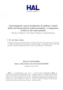
sensor deployment, road location and region specification for real experiment
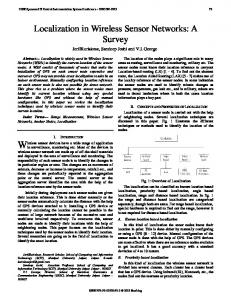
Region 1, sensitivity = 90%, specifity = 81%.
100
2 acoustic
sensor location road location
1
50
0 region 1 42 58
56 52
50
20
40
60
80
100
120
140
160
180
0
20
40
60
80
100
120
140
160
180
0
20
40
60
80
100
120
140
160
180
0
20
40
60 80 100 120 time steps, 1 step stands for 0.75 sec
140
160
180
1
55
53 −50
0
2
41
54
0
51
2
49 47
−100
48
PIR
Y coordinates
region 2
59
seismic
1
0
0
Node 1 is the manager node for region 1 the detection node for region 1 are 41 42 51 54 55 56 59
multi−modality
−150
Node 58 is the manager node for region 2 the detection node for region 2 are 47 48 49 50 52 53 −200 −200
−150
−100
−50 0 X coordinates
1
50
100
1
0.5
0
150
Fig. 1. sensor deployment, road coordinate and region specification for experiments
Fig. 2.
Multi-modality region detection for region 1 (AAV) Region 2, sen = 76%, specifity = 100%. acoustic
2
IV. E XPERIMENTS
1
0
0
20
40
60
80
100
120
140
160
180
0
20
40
60
80
100
120
140
160
180
0
20
40
60
80
100
120
140
160
180
0
20
40
60 80 100 120 time steps, 1 step stands for 0.75 sec
140
160
180
seismic
2
1
0
PIR
2
1
multi−modality
0 1
0.5
0
Fig. 3.
Multi-modality region detection for region 2 (AAV)
announces the target detection. Sensitivity is detection rate when the targets are in the region. We also compute the localization errors defined as the Euclidian distance between the location estimates and the true target locations for all time instant when region detection is announced. The true target location can be determined since they must be positioned on the target trajectory which can be extracted from GPS log. These localization errors are then grouped into different error range, i.e., 0 ∼ 10, 10 ∼ 20, ...40 ∼ 50, ≥ 50. We call it as error histogram of our localization algorithm. Fig. 5 shows this localization error histogram for AAV localization. Raw acoustic, seismic and PIR signatures were also recorded for DW vehicle in the experiments. Using the same sensor network system and collaborative source localization
experiment for aav3 single target localization 60
40
ground truth NLS ML road coordniates
miss detection, so localization is not active here
20
0 Y coordinate
The raw signals were recorded by 29 sensor nodes deployed along the road in the sensor field, CA in November 2001, sponsored by the DARPA ITO SensIT project. Each sensor node is composed of a palm with wireless ratio link, an acoustic sensor, a seismic sensor, a PIR sensor and three coaxial cables which connect the sensors to the palm. The data we used to evaluate our collaborative source localization algorithms were taken from 15 sensor nodes recording the acoustic, PIR and seismic signatures of AAV vehicle going from east to west during a time period of 2 minutes. Figure 1 shows the road coordinates and sensor node positions, both supplied by the global positioning system (GPS). The sensor field is divided into two regions as shown in the above figure. Region 1 is composed of node 1, 41, 42, 46, 48, 49, 50, 51. Region 2 is composed of node 52, 53, 54, 55, 56, 58, 59. In region 1, node 1 is chosen as manager node, others are detection node. In region 2, node 58 is chosen as manager node, others are detection node. The sampling rate is fs = 4960Hz. The energy is computed by averaging the T=0.75sec non-overlapping data segment (3720 data points). Fig. 2 and Fig. 3 show the multi-modality node detection results for acoustic, seismic and PIR modality and the multimodality region detection results. The constant C we choose for the CFAR detector are C = [3.5, 5, 10] for acoustic, seismic and PIR respectively. α = 0.99 for all of the three modality CFAR detector. The weights we used for the region fusion decision of the acoustic modality, seismic modality and PIR modality are 0.3, 0.5, 0.2 respectively. If the region fusion result is bigger than or equal to 0.5, manager node announces the target. Fig. 4 shows the AAV ground truth and the localization results based on the ML algorithm with projection solution and NLS algorithm. MR search is used to estimate the location. The grid size we chose is: 4*4, 2*2, 1*1. Note that the missing ground-truth points in this figure are the miss-detection points by our multi-modality detector and therefore, there is no localization operation at these points. To evaluate this collaborative source localization algorithms, we define the specifity and sensitivity parameters to indicate the performance of region detection. Specifity is the rate which denotes the correct announcement percentage when the region
−20
−40
−60
−80
−100 −100
−50
0
50
100
150
X coordinate
Fig. 4. AAV ground truth and localization estimation results based on ML algorithm with projection solution and NLS algorithm (MR search is used, grid size is 4*4, 2*2 and 1*1. Estimation results look bias from the ground-truth, see discussion for reasoning)
histogram of localization err for NLS and ML estimation for aav3 experiment 35
number of estimation points within the coresponding error range
NLS ML 30
25
20
15
10
5
0
Fig. 5.
10
20 30 40 estimation error range (m), 0~10,10~20,20~30,30~40,40~50,>=50
50
Estimation error histogram for AAV experiment data experiment for dw6 single target localization 60
40
ground truth NLS ML road coordniates
V. C ONCLUSION
20
Y coordinate
0
−20
−40
−60
−80
−100
−120 −100
−50
0
50
100
150
X coordinate
Fig. 6. DW ground truth and localization estimation results based on ML algorithm with projection solution and NLS algorithm (MR search is used, search grid size is 4*4, 2*2 and 1*1. Estimation results look bias from the ground-truth, see discussion for reasoning)
algorithms, we get the localization results and localization error histogram for DW data. They are shown in Fig. 6 and Fig. 7. 1) discussion: From experiment, we can see that this new collaborative source localization algorithm is robust and accurate most of time. The specifity and sensitivity parameters are high. Both ML and NLS algorithms perform well estimations of target location when the targets are detected to be in the region. ML algorithm with projection solution outperforms to NLS algorithm in the sense that it has less estimation error. Besides, there are some points having estimation error bigger than 50 meters using NLS estimation. This says that NLS is not as stable as ML estimation with projection solution. However, NLS algorithm needs less bandwidth. This is because histogram of localization err for NLS and ML estimation for dw6 experiment 18
number of estimation points within the coresponding error range
NLS ML 16
14
12
10
8
6
4
2
0
Fig. 7.
NLS doesn’t use noise variance for its estimation while ML algorithm does need it. So, for NLS algorithm, we save about 1/4 bandwidth. (For ML estimation, detection nodes need to report acoustic energy, noise mean, noise variance and multimodality binary node detection results in every 0.75 second). Fig. 4 and Fig. 6 show that the localization estimation results look bias from the real ground-truth. This might be caused by uncorrected GPS position reports, un-calibrated sensor gain, incorrect background noise estimation or some individual sensor fault measurements. It can be seen that both AAV and DW ground truth also look bias from the road while in the experiment, they moved along the road. We can also see that estimation results are closer and less biased to the road than to the ground-truth.
10
20 30 40 50 60 estimation error range (m), 0~10,10~20,20~30,30~40,40~50,>=50
Estimation error histogram for DW experiment data
Collaborative energy-based source localization method has been presented. Experiments show that this new approach is robust and accurate most of time. Besides, this new approach needs low communication bandwidth since the algorithm is activated only the region is activated. In addition, each sensor only reports energy reading, noise mean and variance ( NLS doesn’t need variance), and detection binary results to the manager node at every time period rather than at every time instant. Besides, it is power efficient. For detection node, it only calculates the average energy in the time period and performs energy-based CFAR detector (simple algorithm). For manager node, it performs simple voting algorithm and decision fusion algorithm. Manager node performs localization algorithm only if the region detection announces the targets. ML estimation with projection solution and MR search under the reduced search region saves the computation burden and so, saves the manager node battery further more. Detection node energy computation requires averaging of instantaneous power over a pre-defined time interval. Hence it is less susceptible to parameter perturbations, and so, the algorithm is robust. R EFERENCES [1] Estrin, D., Culler, D., Pister, K., and Sukhatme, G.,: Connecting the Physical World with Pervasive Networks, IEEE Pervasive Computing, 1, Issue 1, (2002), 59-69 [2] Savarese, C., Rabaey, J. M., and Reutel, J.: Localization in distributed Ad-hoc wireless sensor networks, Proc. ICASSP’2001, Salt Lake City, UT, (2001), 2037-2040 [3] Oshman, Y., and Davidson, P., Optimization of observer trajectories for bearings-only target localization, IEEE Trans. Aerosp. Electron., 35, issue 3, (1999), 892-902 [4] Kaplan, K. M., Le, Q., and Molnar, P.,: Maximum likelihood methods for bearings-only target localization, Proc IEEE ICASSP, 5, (2001), 30013004 [5] Carter G. C.,: Coherence and Time Delay Estimation, IEEE Press, 1993. [6] Yao, K., Hudson, R. E., Reed, C. W., Chen, D., and Lorenzelli, F.,: Blind beamforming on a randomly distributed sensor array system, IEEE J. Selected areas in communications, 16 (1998) 1555–1567 [7] Reed, C.W., Hudson, R., and Yao,K.,: Direct joint source localization and propagation speed estimation. In Proc. ICASSP’99, Phoenix, AZ, (1999) 1169-1172 [8] Special issue on time-delay estimation, IEEE Trans. ASSP 29, (1981) [9] Sheng, X., Hu, Y. H.,: Energy based source localization, to appear IPSN2003.