Feb 2, 2008 - previous work [43â45], and we present a new result for the fully ...... To investigate the oscillations of the degree of freedom physically described ...
Collective dynamics of internal states in a Bose gas ¨ Oktel† , L. S. Levitov M. O. Department of Physics, Massachusetts Institute of Technology, Cambridge, MA 02139
arXiv:physics/0108052v1 [physics.atom-ph] 27 Aug 2001
February 2, 2008 Theory for the Rabi and internal Josephson effects in an interacting Bose gas in the cold collision regime is presented. By using microscopic transport equation for the density matrix the problem is mapped onto a problem of precession of two coupled classical spins. In the absence of an external excitation field our results agree with the theory for the density induced frequency shifts in atomic clocks. In the presence of the external field, the internal Josephson effect takes place in a condensed Bose gas as well as in a non-condensed gas. The crossover from Rabi oscillations to the Josephson oscillations as a function of interaction strength is studied in detail.
PACS numbers: 03.75.Fi, 05.30.Jp I. INTRODUCTION
Recent experiments achieving the trapping and Bose condensation of atoms with hyperfine structure [1–7] have created a lot of theoretical interest in the behavior of atomic gases with internal degrees of freedom [8–15]. Most of this interest has focused on how the presence of internal degrees of freedom effect the spatial behavior, such as the hydrodynamical modes or vortices. An equally important question posed by these experiments is how the internal states of the atoms are effected by interactions. In a variety of experiments the transitions between internal states are used to either manipulate or probe cold gases. Fountain atomic clocks [16–19] use Ramsey spectroscopy technique to measure the energy differences between internal states very precisely, and have found that this energy difference depends on the densities of the different internal states in the gas. Another class of experiments have used Electromagnetically Induced Transparency [20] techniques to excite the atoms into a superposition of internal states by absorbing a ‘probe’ beam and were able reemit the beam after some delay. These experiments measured the change in the ‘stopped’ light beam as the gas evolved in the superposition state [21,22]. Both of these classes of experiments measure the internal dynamics of the atoms in a normal gas. Experiments involving change in the internal state of the atoms have also been carried out on Bose Einstein Condensates (BEC). In the MIT spin polarized Hydrogen experiment [23,24], BEC was detected by changing the internal states of the atoms from 1S to 2S using a two photon excitation. Two photon transitions have also been successfully employed by the JILA group in a number of experiments to create topological excitations [25,26] or phase textures [27] in a Rubidium BEC. One can expect many related experiments to be carried out in near future as the study of cold atomic gases is a rapidly expanding field. Although all these experiments try to elucidate the internal dynamics of a cold gas, it is useful to classify them into two groups with respect to the strength of the external field that couples to the internal states. In the weak field limit, experiments probe the internal dynamics of a gas of atoms in the absence of an external field. For example, in the atomic clock experiments, although strong fields at the beginning and the end of Ramsey spectroscopy are required, an essentially free evolution of the wavefunction in a superposition of two internal states is measured. In the MIT hydrogen experiment [23], the number of excited atoms is a small fraction of the total number, and thus all the effects measured are linear in the excitation rate. Thus the external field is only a weak probe of the free dynamics. On the other hand, in the strong field limit the internal dynamics is sensitive to the intensity of the external field, and the number of atoms changing their internal state form a large fraction that may reach 100%. In the JILA experiments, by applying a π pulse all the atoms are transferred from one internal state to the other, and duration of the pulse is the inverse of Rabi frequency, showing that the internal dynamics depends on the strength of the external field. It should be also kept in mind that in all these experiments, even in the weak field limit, the external field has large enough number of quanta to be treated as a classical field. Also we will assume throughout that the excitation is carried out by a coherent field. The interaction between two atoms generally depends on their internal states [28,29]. For the dilute cold gases considered in this work, interactions can be simply characterized by the s-wave scattering lengths aαβ which depend on the internal states α and β of the interacting atoms. Thus a two state problem will have three different scattering lengths. To be in the purely s-wave scattering limit the gas has to be cold enough, so that a ≪ 1, λT
1
(1)
where a is the largest of the s-wave scattering lengths in the problem and λT = h(2πmkb T )−1/2 is the thermal de Broglie wavelength. The temperature range defined by the criterion (1) corresponds to the so-called cold collision regime. It is important to realize that the inequality (1) not only defines the condition for the s-wave scattering to be dominant, but also is a criterion for quantum statistical effects (indistinguishibility of the particles) to be observable. To see this, consider an evolution of the state of one particular atom. This atom will experience two different kinds of scattering processes: the coherent forward and backward scattering which preserves correlation of the momentum state with the internal state, as well as ordinary elastic collisions causing scattering at an angle different from 0 or π which destroy this correlation [30,31]. The forward and backward processes occur with the ‘rate’ −1 τcoh =
4π¯ha n, m
(2)
while the ordinary elastic collisions rate is −1 τcoll = 4πa2 nvT ,
(3)
p where vT = 2kB T /m is the thermal velocity. Comparing these two rates one can see that the coherent processes happen at a much higher rate in the temperature range (1). It is then possible to measure the frequency shifts of the internal states and decide the statistics of the system. The gases satisfying the condition (1) are called quantum gases [30–33]. For the densities relevant for the alkali gas experiments, the temperatures below which the gas becomes quantum in the sense (1) are much larger than the Bose-Einstein condensation temperature. [This is true because quantum degeneracy becomes important only at the lower temperatures for which the thermal de Broglie wavelength is the order of average interparticle spacing, λT ≃ n−1/3 .] For Bose systems the substantial overlap between wavefunctions of different particles and bosonic tendency to be in the same state then causes Bose–Einstein condensation, where a finite fraction of the particles of the gas share the same spatial wavefunction. The internal states of the particles define the interactions between the particles, thus determine the self-consistent spatial wavefunction that all the particles share [1,3], transition between internal states are also effected in return. Most importantly, there are no backward(exchange) scatterings between two bosons sharing the same spatial wavefunction, and the mean field energy shift for a particle in the condensate is different from a particle in the normal gas. An important example of the modification of the transitions between the internal states upon condensation is given by the internal Josephson effect [34–38,29]. In this effect, the internal states act as the two reservoirs and the external field provides the weak link between these two reservoirs similar to the tunneling coupling through a barrier in the ordinary spatial Josephson effect [39–42]. Although the JILA experiments [2,3] have come close, the internal Josephson effect has not been observed in the alkali gases to date, mostly due to the fact that the shape of the condensate is different for the two internal states. Any transition between the two internal states causes spatial disturbances, making the internal Josephson oscillations hard to observe. It should however be possible observe the effect by either using a very shallow trap or going to the adiabatic limit in which the Rabi frequency for transitions is much larger than the oscillation frequencies of the condensate in the trap [34,29]. We will consider the case of a homogeneous gas and investigate the Internal Josephson effect, having in mind a gas sample in a very shallow trap. To understand these different phenomena in a general framework, we first derive the transport equation for the density matrix of the system, treating the external degrees of freedom semi–classically. The transport equation can be used to understand transitions between internal states of a Bose gas in the presence of spatial non-uniformity caused by a trapping potential, as well as in the presence of macroscopic flows, such as currents created by a vortex. Below we focus on the dynamics of internal states in a spatially uniform system. We assume that all the excitation fields are applied uniformly on a homogeneous sample. We find the equations of motion for the internal state density matrix of both the normal component and the condensed part of a Bose gas. Then we use a Bloch sphere representation [46] for the density matrix to get an equivalent equation of motion for classical spins. After deriving the equations of motion we consider two simple cases: a normal gas and a fully condensed gas. We find the free precession frequencies for the relative phase of two internal states, which leads to an expression for the density dependence of the frequency shift in fountain atomic clocks. Our results for the normal gas agree with previous work [43–45], and we present a new result for the fully condensed case. Then we investigate the response of the Bose gas to an external field when it is either above condensation temperature or at zero temperature, i.e. fully condensed. For the fully condensed Bose gas we show how the Rabi oscillations in a non-interacting gas turn into the internal Josephson oscillations, and calculate the oscillation frequencies exactly for the entire parameter range. By repeating the same analysis for a non-condensed gas, we find that the internal Josephson effect exists in a cold non-condensed gas. This somewhat surprising result shows that the Josephson effect does not require a broken symmetry, and can be observed in any coherent system. We calculate the frequencies for 2
the normal case and compare with the results for condensed gas. We also compare the internal Josephson oscillations with the spatial Josephson oscillations discussed in [39–42] and show that ‘macroscopic quantum self trapping’ effect is also present for the internal Josephson effect. In the next section, we study the internal dynamics of a Bose gas which has comparable densities of condensed and normal components. We first discuss the dynamics without an external coupling field and calculate the oscillation frequencies for the condensate density in each internal state. In the limit of small oscillation amplitude out result agrees with the resonance frequencies calculated for the MIT hydrogen spectrum [33]. We briefly discuss the behavior of the system under a strong external field. Finally we give the transport equation and the equations of motion for the internal density matrix of a Fermi gas. We consider a freely precessing state and its response to an external field, and compare the results with those for the Bose gas. II. THE TRANSPORT EQUATION
A dilute Bose gas in a confining potential U (r) can be described by the Hamiltonian � 2 2 � X R ¯h ∇ H = d3 r ψα+ (r) − +h ¯ Uα (r) ψα (r) 2m α X R ¯hλαβ + + d3 r ψα (r)ψβ+ (r)ψβ (r)ψα (r), 2
(4)
α,β
where the Greek indices α, β run over all internal states. The potential energy h ¯ Uα (r) includes the internal energies ¯ wα of the states |αi, h h ¯ Uα (r) = h ¯ U (r) + h ¯ wα , and the interaction parameters λαβ are related to the s-wave scattering lengths aαβ as λαβ =
4π¯h aαβ . m
(5)
For a problem with N internal levels there are N (N + 1)/2 interaction strengths λαβ to be specified. The operators ψ(r) are the canonical second-quantized Bose operators, satisfying [ψα (r), ψβ+ (r′ )] = δαβ δ(r − r′ ).
(6)
Transitions between internal states caused by an excitation field, are described by another term to be added to the Hamiltonian (4): XZ Hexc = d3 rVαβ (r, t)ψα+ (r)ψβ (r). (7) αβ
We assume harmonic time dependence Vαβ (r, t) = Aαβ (r) exp(iΩαβ t)
(8)
where Aαβ (r) is a function of coordinates describing spatial distribution of the excitation field [20]. The requirement ∗ of being hermitian gives Vαβ (t) = Vβα (t). In the case of Bose condensation we can treat the ψ operators as having non-zero expectation values. This is achieved by a substitution ψˆα (r) → ψˆα (r) + ψ¯α (r),
(9)
where ψ¯α is a c-number representing the condensate wavefunction. To describe the dynamics of the internal states of the normal gas, we need the populations of each level, as well as the coherences between any two states. Thus we define the full density matrix ̺(r, p) and the internal density matrix ρ(r), both being N × N hermitian matrices for N internal states: Z ′ r′ r′ ̺αβ (r, p) = d3 r′ hψα+ (r + )ψβ (r − )iei~p·~r (10) 2 2 Z d3 p ̺αβ (r, p) = hψα+ (r)ψβ (r)i. ραβ (r) = (2π)3 3
The internal dynamics of the condensate can be described by specifying complex amplitudes of internal states, in total N complex numbers for an N component condensate. We find it useful, in order to keep track of relative phases of condensate internal states, to introduce an N × N matrix similar to the density matrix of normal states ρ¯αβ (r). We will also need to keep track of the condensate flow described by J~αβ . These quantities are defined as ρ¯αβ (r) = ψ¯α∗ (r)ψ¯β (r) � h � ¯∗ ¯ J~αβ (r) = i (∇ψα (r))ψ¯β (r) − ψ¯α∗ (r)(∇ψ¯β (r)) . 2m
(11)
Here one notes that ρ¯ is always rank one, thus the matrix does not contain any additional information but is introduced just for convenience. The diagonal elements of ραα (r) and ρ¯αα (r) give the thermal and condensate populations ntα (r) and ncα (r), respectively. Total density of atoms in state |αi is nα (r) = ntα (r) + ncα (r). We start with deriving the equations of motion for ̺ and ρ¯. Using the Heisenberg equations of motion for the field operators d ψα (r) = i[H, ψα (r)], dt ∂H d ¯ ψα (r) = i ¯∗ dt ∂ ψα (r)
(12)
dρ¯ and then taking the required expectation values we obtain d̺ dt (r, p) and dt (r). The contribution of each term in the Hamiltonian to the evolution of ̺ and ρ¯ can be evaluated separately. To remind the reader how this calculation is carried out we present the contribution of potential energy to d̺ dt (r, p). First we calculate "Z # X 3 ′ ′ + ′ ′ ψ˙ α (r) = i d r Uγ (r )ψ (r )ψγ (r ), ψα (r) (13) γ
γ
=i
Z
d3 r′
X
Uγ (r′ )[ψγ+ (r′ ), ψα (r)]ψγ+ (r′ )
γ
= −iUα (r)ψα (r). Upon complex conjugation we get ψ˙ α+ (r) = iUα (r)ψα+ (r). Then we write the contribution of potential energy to d̺ dt (r, p) as Z � � ′ (Pot) ̺˙ αβ (r, p) = d3 r′ eip·r hψ˙ α+ (r + r′ /2)ψβ (r − r′ /2)i + hψα+ (r + r′ /2)ψ˙ α (r − r′ /2)i � � Z ′ Uα (r) + Uβ (r) ≃ i d3 r′ eip·r Uα (r) − Uβ (r) + ~r′ · ∇r ( ) hψα+ (r + r′ /2)ψβ (r − r′ /2)i 2 Uα (r) + Uβ (r) = i(Uα (r) − Uβ (r))̺αβ (r, p) + ∇r ( ) · ∇p ̺αβ (r, p). 2
(14)
(15)
Going through this procedure for each of the terms in the Hamiltonian we get the equation of motion. Whenever we need to calculate the expected value of a 4 particle operator we do it using Wick’s theorem, hψα+ ψβ+ ψβ ψα i = hψα+ ψα ihψβ+ ψβ i + hψα+ ψβ ihψβ+ ψα i.
(16)
In this averaging the first term is referred to as the direct (Hartree) term as it depends only on densities while the second is the exchange (Fock) term that involves coherences. We find the following equations describing the space and time variation of the two matrices: � � p ~ Uα (r) + Uβ (r) (17) ∂t + · ∇r − ∇r ( ) · ∇p ̺αβ (r, p) = m 2 " # X tot + i Uα (r) − Uβ (r) + (λγα − λγβ )ργγ (r) ̺αβ (r, p) γ
4
+i
X γ
+
λγα ρtot αγ (r)̺γβ (r, p) − i
X λγα + λβγ 2
γ
+
X λγα 2
γ
+i
X γ
+
X
λβγ ρtot γβ (r)̺αγ (r, p)
γ
∇r ρtot γγ (r) · ∇p ̺αβ (r, p)
∇r ρtot αγ (r) · ∇p ̺γβ (r, p) −
X λβγ 2
γ
∇r ρtot γβ (r) · ∇p ̺αγ (r, p)
[Vγα (r, t)̺γβ (r, p) − Vβγ (r, t)̺αγ (r, p)]
1X [∇r Vγα (r, t) · ∇p ̺γβ (r, p) − ∇r Vβγ (r, t) · ∇p ̺αγ (r, p)] 2 γ
and � � ∂t ρ¯αβ (r) + ∇r · J~αβ (r) = " # X tot + i Uα (r) − Uβ (r) + (λγα − λγβ )ργγ (r) ρ¯αβ (r)
(18)
γ
+i
" X γ
+i
X γ
λγα ραγ (r)¯ ργβ (r) −
X
#
λβγ ργβ (r)¯ ραγ (r)
γ
[Vγα (r, t)¯ ργβ (r) − Vβγ (r, t)¯ ραγ (r)]
where ρtot (r) = ρ(r) + ρ¯(r). Let us summarize here the approximations used to derive the above equations and assess their validity. The HartreeFock approximation is used to treat interactions, that is the same as keeping the lowest order term in the expansion in the gas parameter na3 . This is an excellent approximation for the dilute atomic gases where na3 is usually about 10−6 . The most important restriction on the above equations (17,18) is that they are valid for times not longer than the elastic scattering time −1 τcoll = 4πa2 nvT .
(19)
−1 However, for a cold gas the characteristic frequency of the evolution described by (17,18) is much higher than τcoll , and this approximation gets better as the temperature is decreased. The decoherence due to elastic collisions can be described heuristically by adding a damping term (Damp)
̺˙ αβ
= −4πa2αβ vT ̺αβ (1 − δαβ ),
(20)
on the right hand side of Eq.(17). All other effects, such as the difference of the trap potential for different internal states, or density oscillations created by a change in the internal state are adequately described by (17,18) within the Hartree-Fock approximation. III. EQUATION OF MOTION FOR THE INTERNAL DENSITY MATRIX
Our main interest in this paper will be the consequences of interparticle interactions in the internal state dynamics, so we will simplify the above general equations by assuming that we are in a uniform system, with no normal or condensate flows, and further assume that the external fields are applied uniformly. In this case we will have no need for the full density matrix ̺(r, p), as internal dynamics is completely described ρ(r) which will be the same at all points r. Thus equations of motion reduce to X ρ˙ γγ ′ = i(wγ − wγ ′ + Uγ − Uγ ′ )ργγ ′ + i (21) λαγ (ργα + ρ¯γα )ραγ ′ α
−i
X
λαγ ′ (ραγ ′ + ρ¯αγ ′ )ργα + i
α
X α
5
(Vαγ (t)ραγ ′ − Vγ ′ α (t)ργα )
ργγ ′ + i ρ¯˙ γγ ′ = i(wγ − wγ ′ + Uγ − Uγ ′ )¯ −i
X
λαγ ′ ραγ ′ ρ¯γα + i
α
X
λαγ ργα ρ¯αγ ′
(22)
α
X ργα ) (Vαγ (t)¯ ραγ ′ − Vγ ′ α (t)¯ α
where Uγ are defined as, Uα =
X
λαβ (ρββ + ρ¯ββ ) =
β
X
λαβ nβ .
(23)
β
The dynamics described in the above equations are fairly complicated if there are fields coupling more then two states, so we will concentrate on the simplest case, where only two internal states are coupled, and all the populations in the other states remain constant. In this case we will be concerned with the dynamics of two, two by two matrices. One for the normal gas and one for the condensate. Let us assume that states 1 and 2 are coupled. We can go to a Larmor basis with the frequency of the coupling field so that the elements of our density matrix (and similarly the condensate matrix) can be redefined. The diagonal elements of the matrices do not change while the off-diagonal elements change as ρ′21 = (ρ′12 )∗ .
ρ′12 = ρ12 exp[−iΩ12 t],
(24)
In this basis we will find it useful to rewrite the equations of motion in the Bloch representation [46]. Being 2 by 2 hermitian matrices we can expand, ~ · ~σγγ ′ ρ′γγ ′ = ρ0 δγγ ′ + S ~c · ~σγγ ′ ρ¯′ γγ ′ = ρ¯0 δγγ ′ + S
(25)
where ~σ are the Pauli matrices. In this representation ρ¯0 and ρ0 will be proportional to the total number of atoms in the condensate, and above the condensate respectively. The z components of both spins are proportional to the population difference between the two internal states, belonging to the normal gas or the condensate. For the normal part, the norm of the projection of spin onto the x − y plane represents the degree of coherence between the two internal states. For the condensate spin however, this norm is directly proportional to the geometric mean of the populations of the two internal states. The angle corresponding to a rotation around the z axis is related to the relative phase of the two internal states, in both cases. The matrix Vαβ has no diagonal elements as defined in the excitation Hamiltonian. However, we can take the detunings that come as a result of going to Larmor basis, as the diagonal elements. V11 (V22 ) being defined as +(−)[w2 − w1 − Ω12 ]. Then we can again expand Vγγ ′ as ~ · ~σγ ′ γ . Vγγ ′ = V0 δγγ ′ + V
(26)
In this representation we can write the equations of motion for the condensate and the normal gas spins as : ~ ×S ~ c + 2S ~×V ~ ~˙ = S ~ ×B ~ n + 2λ12 S S ~c × S ~ + 2S ~c × V ~ ~˙c = S ~c × B ~ c + 2λ12 S S
(27)
with, ~ n = [(λ11 − λ22 )(2ρ0 + ρ¯0 ) + (λ11 + λ22 − 2λ12 )(2S ~ +S ~c ) · zˆ]ˆ B z ~ ~ ~ Bc = [(λ11 − λ22 )(ρ0 + ρ¯0 ) + (λ11 + λ22 − 2λ12 )(S + Sc ) · zˆ]ˆ z.
(28)
It is important to observe that the equations conserve the total densities in the condensed and non condensed fractions of the gas. To get a better sense of the equations we can note that they can be derived from the XXZ self interacting Hamiltonian: ~ +S ~c ) + (λ11 − λ22 )ρ0 zˆ · S ~ H = (λ11 − λ22 )(ρ0 + ρ¯0 )ˆ z · (S 1 +J ij S i S j + J ij Sci Scj + J ij Sci S j 2 ~ +S ~c ).V ~ +2(S 6
(29)
where,
using the Poisson spin algebra:
2λ12 0 0 0 J = 0 2λ12 0 0 (λ11 + λ22 )
(30)
{S i , S j } = ǫijk S k {Sci , Scj } = ǫijk Sck {S i , Scj } = 0.
(31)
Let us briefly remind what the physical bases for various terms in the Hamiltonian are. The factor of 2 difference in the normal spin–normal spin interaction compared to the condensate spin–condensate spin interaction stems from the fact that there are no exchange scatterings within the condensate. The terms coupling the condensate spin with the normal spin arise from processes in which an atom in one internal state goes through an exchange scattering process with a condensate atom in another internal state. IV. DENSITY SHIFTS IN ATOMIC CLOCKS: FREE PRECESSION OF A SINGLE SPIN
We start the analysis of the dynamics described in Eq.(27) by considering the situation in which we can represent the system by a single spin. There are two such cases. The first is at zero temperature, when almost all the atoms are in the condensate; while the second is above the transition temperature, when there is no condensate present. However, our analysis is still restricted to temperatures low enough to satisfy the quantum gas condition, λT > as . We first analyze equations of motion Eq.(27) in the case where there is no external field. Such an analysis is needed to understand any interaction related effects in experiments where particles spend a substantial amount of time in a superposition state, such as atomic clocks [16–19]. Let us first consider the case where there is no Bose condensation. Thus our equations (27) will be reduced to ~ =S ~ ×B ~ n. S
(32)
We can easily see that the z component of the spin will be conserved and we will only have a precession around the z axis and the precession frequency will be X ω = (w2 − w1 ) + 2(λ22 n2 − λ11 n1 + λ12 (n1 − n2 )) + (λ2γ − λ1γ )nγ . (33) γ6=1,2
This result agrees with the theory of frequency shifts in atomic clocks [43–45]. We can now ask the same question for a sample which is fully condensed. When all the atoms are in the condensate, they will all be sharing the same spatial wavefunction, this will mean that no exchange processes will be possible. That would eliminate the factor of 2 multiplying the combination of λ and n’s for states one and two in the previous equation. Not surprisingly we get, for a fully condensed sample X ω = (w2 − w1 ) + (λ22 n2 − λ11 n1 + λ12 (n1 − n2 )) + (λ2γ − λ1γ )nγ . (34) γ6=1,2
Although it is not desirable to use a condensate in a fountain atomic clock due to very high density shifts that would result. We see here that such an experiment can be used to probe the correlations in a condensate by simply looking at the density induced frequency shifts. V. INTERNAL JOSEPHSON EFFECT: SINGLE SPIN UNDER AN EXTERNAL FIELD
In this section we consider the response to an external field, only when the system can be represented by a single spin, i.e. the system is either fully condensed or not condensed at all. In the former case, when the system is at zero temperature we have two condensates in internal states 1 and 2, which are connected by the “weak link” supplied by the external field. This is the well studied problem of the internal Josephson effect [34–38]. 7
The important difference between the spatial Josephson problem and the internal Josephson problem is that in the latter atoms in different internal states interact, while in the former two particles in different reservoirs do not. However if the interaction between the two internal states is taken to be zero λ12 = 0,
(35)
then equations for the internal Josephson problem reduce to that of the spatial problem [40–42]. thus the internal effect displays all the phenomena the spatial Josephson effect has. As in the spatial Josephson problem there are three different regimes depending on the strength of the coupling between the internal states [29]. If the external field is much stronger than the interactions ~ | ≫ λn, |V
(36)
the system is said to be in the Rabi regime. (Here λ can be taken to be the largest of λαβ and n the total density.) In this regime interactions are not important and the system experiences large oscillations in the density of each internal state. In the opposite regime, when the external field is extremely weak, ~ | ≪ λn, |V
(37)
the system is in the Fock regime. The amplitude of density oscillations is negligible and the phase difference between the two states evolves as in the free precession case discussed in the previous section. Between these two regimes is the Josephson regime, for which, ~ | ∼ λn. |V
(38)
In this regime, the density imbalance between the two internal states go through small oscillations, similar to the usual spatial Josephson effect. All three regimes are described by Eq.[27], which reduces to ~˙c = S ~c × B ~ c + 2S ~c × V ~ S ~ c = [(λ11 − λ22 )ρ0 + (λ11 + λ22 − 2λ12 )S ~c · zˆ]ˆ B z,
(39)
at zero temperature. As the dynamics conserves the magnitude of the spin we only have two dynamical variables, which can be taken as angles (θ, φ) in the spherical polar coordinates representing the orientation of the spin. Another conserved quantity in this dynamics is the Hamiltonian introduced earlier, ~c · V ~. ~c + 1 J ij Sci Scj + 2S H = (λ11 − λ22 )¯ ρ0 zˆ · S 2
(40)
On the sphere defined by (θ, φ), contours of constant H will define the paths along which the spin will precess. We can write the Hamiltonian as a function of (θ, φ) as H = A cos2 (θ) + B cos(θ) + C sin(θ) cos(φ) + D,
(41)
and identify 1 (λ11 + λ22 − 2λ12 )|Sc |2 2 B = ((λ11 − λ22 )¯ ρ0 |Sc | + 2V z |Sc |) C = 2V x |Sc | D = λ12 |Sc |2 . A=
(42)
~ , passing At strong external fields the paths are almost circular with centers on the line oriented along vector V through the origin, as in the usual Rabi problem, and significant changes in the populations occur throughout the course of a Rabi oscillation. As a function of θ and φ the Hamiltonian has one maximum and one minimum, thus all the trajectories circle these extremum points, if the external field satisfies 2/3 C > (1 − B )3/2 . (43) 2A 2A 8
~ | becomes the order of the density caused shifts ∼ λn, We get into the When the intrinsic Rabi frequency |V Josephson regime. Even on resonance, large population transfers from one state to another does not take place. This can be easily seen from the structure of trajectories on the Bloch sphere. When the external field does not satisfy (43), instead of having one minimum and one maximum, the Hamiltonian has two maxima, one minimum and a saddle point. The two constant H trajectories crossing at the saddle point separate the sphere into three regions, giving us three kind of trajectories, circling around the minimum or one of the two maxima. None of these oscillations however, result in large population transfers, which is in contrast with the Rabi problem, in which one can change internal states of all the atoms with an arbitrarily small field on resonance. Josephson effect can be understood if we realize that the transition frequency for an atom depends on the populations. So for weak fields even a small population transfer carries the transition away from resonance, i.e. makes the effective detuning much larger than the Rabi frequency. We can calculate the oscillation frequency along each path, for both high and low fields. The period of the precession along a path C on which H(θ, φ) = H′ is given by Z 1 ′ . (44) dl T (H ) = |∇H| C By converting the integral to a surface integral over a δ function and integrating over the angle φ, we have Z 1 2 dx √ 4 T = 3 |A| x + C3 x + C2 x2 + C1 x + C0
(45)
where B C3 = 2 � �A 2 H−D C + B2 − 2 C2 = A2 A B(H − D) C1 = −2 A2 2 C − (H − D)2 . C0 = − A2
(46)
In the high field case, for the external field satisfying (43), the Hamiltonian will take values between Hmax and Hmin , the values of the Hamiltonian at the maximum and minimum points. Any value of H in this range will uniquely correspond to one trajectory and the period of motion on such a trajectory will be given by s 4 1 (x1 − x2 )2 − (p − q)2 T = ) (47) √ K( |A| pq 2 pq p2 = (m − x1 )2 + n2 q 2 = (m − x2 )2 + n2
where K is the complete elliptic integral [47], x1 , x2 are the real roots, m is the real part and n is the absolute value of the imaginary part of the remaining two complex conjugate roots of the polynomial in Eq.(45). In the weak field case there are 4 special values of the Hamiltonian, Hmin , the minimum value, Hsaddle the value at the saddle point, Hmax1 and Hmax2 , the smaller and the larger of the values at the two maxima respectively (See Figure 1). For H values in the range Hmax2 > H ′ > Hmax1 or Hsaddle > H > Hmin there is again one to one correspondence between H values and trajectories on the sphere. For such trajectories the frequencies are again given by (47). For the values of H satisfying Hmax1 > H > Hsaddle there are two trajectories corresponding to each H, one circling around Hmax1 , and the other circling around Hmax2 . However they both have the same period given by s (x2 − x1 )(x4 − x3 ) 4 p ) (48) K( T = (x4 − x2 )(x3 − x1 ) |A| (x4 − x2 )(x3 − x1 )
where K is again the complete elliptic integral and x1 < x2 < x3 < x4 are the four real roots of the polynomial in Eq.(45). A typical plot of frequencies for the weak field case is given in figure 2. Near the saddle point trajectories slow down logarithmically in H − Hsaddle as expected from a two dimensional dynamics. 9
We can see for λ11 = λ22 that our equations reduce to those obtained in [34,41] by using two coupled GrossPitaevskii equations. At high field we get almost circular trajectories, and correspondingly large oscillations between internal levels of the condensate, as in the Rabi problem. For the low field case we get three kind of trajectories all of which give little population change, these correspond to Josephson oscillations. Two of these three kinds complete a full cycle around the z axis, while the third is trapped in a region for which φmin < φ < φmax . Recalling that φ represents the relative phase of the two condensates, we see that these trajectories correspond to Josephson oscillations between the two internal states, caused by the weak link of the external field. The other two kinds of trajectories again correspond to Josephson oscillations, however in these class of Josephson oscillations there is a 2π phase slip for every period of population change. such oscillations are called π Josephson oscillations [42]. It has been shown for the spatial Josephson effect that the system can dynamically maintain a population imbalance between the two macroscopically occupied states [42]. We can ask whether the internal Josephson effect also shows this “macroscopic quantum self trapping” effect. This question is meaningful only if a symmetry exists between states 1 and 2 λ11 = λ22 .
(49)
If the internal states have different interactions a population imbalance is to be expected in any oscillation as the system will be biased to choose the internal state with lower interaction energy. If we take λ11 = λ22 , our condition for the appearance of the extra maximum in the Hamiltonian becomes |C| > 2|A|,
(50)
as B = 0 in this case. One can immediately see that out of the three types of trajectories discussed for the general case, those corresponding to π Josephson oscillations become macroscopically self trapped oscillations for λ11 = λ22 . It is remarkable that none of the arguments given for the internal Josephson effect depend on the macroscopic occupation of a spatial state, i.e. Bose condensation. In fact if we assume that the system is not condensed T > Tc ,
(51)
we get the equation for the precession of the normal spin from Eq.(27) ~˙ = S ~ ×B ~ n + 2S ~×V ~ S ~ n = [(λ11 − λ22 )2ρ0 + (λ11 + λ22 − 2λ12 )2S ~ · zˆ]ˆ B z.
(52)
This equation is very similar to the equation for the condensate spin, and all the results found in this section apply for the non-condensed case if we identify A = (λ11 + λ22 − 2λ12 )|S|2 B = (2(λ11 − λ22 )ρ0 |S| + 2V z |S|) C = 2V x |S| D = 2λ12 |S|2 .
(53)
The behavior of the fully condensed and non-condensed cases are similar, however the values of the precession frequencies and critical value of the external field are different. This difference, again, is a result of the fact that there are no exchange scattering processes in a Bose condensate. From the above discussion we come to the conclusion that to observe the internal Josephson effect it is not required to have two Bose condensed samples. Two words of caution should be voiced about this observation. First we have only considered the coherent collisions and the coherence of the phase of two internal levels will be destroyed on a time scale that is set by mean free time in the gas. Any observed internal Josephson oscillation in a non-condensed sample should decay in this time scale. Second, to be able to see this effect one has to go to very low field strengths such that the population oscillations should be observable in a non-condensed sample. Still we have shown that it is not absolutely necessary to have Bose condensation to observe small oscillations in the relative phase of the internal states under a small excitation field. Let us imagine a non-condensed gas of atoms put into a superposition of two internal states by a π/2 pulse. If this sample is further subjected to weak mixing field on resonance one would naively expect population transfer from one internal level to the other with the Rabi frequency of the field. However our discussion shows that if the sample and the field satisfy −1 ~ | ≪ λn τcoll = 8πa2s nvT ≪ |V
(54)
we would have small oscillations of the phase and populations, which is exactly what is observed in the internal Josephson effect with condensed samples. 10
VI. ABSORPTION RESONANCES FOR A PARTIALLY CONDENSED GAS: THE TWO SPIN PROBLEM
After analyzing the fully condensed and non-condensed Bose gas, both of which can be represented by only one spin in our equations (27), we turn our attention to the partially condensed Bose gas. When the temperature is between zero and condensation temperature, TBEC , there is both a condensed and a non-condensed density present. If these densities are comparable we have to use the full form of Eq.(27), with both spins present. We first start with the free precession problem, i.e. by setting the external field equal to zero. In this case we have the equations ~ ×S ~c ~˙ = S ~ ×B ~ n + 2λ12 S S ~c × S. ~ ~˙c = S ~c × B ~ c + 2λ12 S S
(55) (56)
~ n and B ~ c both point in the zˆ direction and are defined in Eq.(28). As their time derivaThe effective magnetic fields B ~ and |S ~c | are conserved. This conservation tives are perpendicular to the spin vectors, norm of both of the spins, |S| simply means that the total number of atoms in the condensate and over the condensate are conserved. Another conserved quantity can be obtained by adding Eq.(55) to Eq.(56) and taking the zˆ component. We have � d � z ~+S ~c ) ≡ d Stot zˆ · (S = 0. (57) dt dt Physically this conservation law corresponds to the fact that in the absence of a coupling field the total number of atoms in internal states 1 and 2 are conserved separately. Although these three conservation laws restrict the resulting dynamics considerably, they still allow oscillations in which the density of condensed and non-condensed atoms in internal state 1 change, while state two goes through the same oscillations out of phase with 1 to leave the total number of condensed and non-condensed atoms constant. In our spin representation the degree of freedom that expresses these oscillations will be S z , or equivalently Scz as they add up to a constant. The other conserved quantity is the Hamiltonian (29) which we choose to rewrite in terms of the conserved quantities z Stot , |S| , |Sc | and the dynamical variable S z as 1 z 2 z ) H = (λ11 − λ22 )(ρ0 + ρ¯0 )Stot + (λ11 + λ22 − 2λ12 )(Stot 2 + 2λ12 |S|2 + λ12 |Sc |2 + (λ11 − λ22 )ρ0 S z 1 ~ · S~c . + (λ11 + λ22 − 2λ12 )(S z )2 + 2λ12 S 2
(58)
To investigate the oscillations of the degree of freedom physically described above and represented by S z we take the equation of motion for S z dS z ~˙ = 2λ12 zˆ · (S ~ ×S ~c ) = 2λ12 V. = zˆ · S dt
(59)
~ and S ~c . We can express the absolute We define V to be the volume of the parallelepiped formed by the vectors zˆ , S value of this volume in terms of the inner products of these three vectors as q ~ ·S ~c )2 − |Sc |2 (S z )2 − |S|2 (S z )2 + 2S z S z S ~·S ~c . (60) |V| = |S|2 |Sc |2 − (S c c
~ ·S ~c in terms of conserved quantities and S z from Eq.(58). This will give us the equation of Now we can solve for S z motion for S expressed only in terms of conserved quantities and S z itself: z dS p z 4 z 3 z 2 z (61) dt = C4 (S ) + C3 (S ) + C2 (S ) + C1 (S ) + C0
The value of S z will oscillate between x1 and x2 which are two roots of the polynomial inside the square root in Eq.(61). For values of S z in the interval x1 < S z < x2 , this polynomial takes positive values. When S z reaches its ~ , S ~c and zˆ are coplanar. This allows us to integrate Eq.(61) without maximum or minimum value, the vectors S paying attention to the absolute value. We can express the period of S z as an integral of the form in Eq.(45) Z x2 1 . (62) dS z p Tz = 2 z 4 z 3 C4 (S ) + C3 (S ) + C2 (S z )2 + C1 S z + C0 x1 11
Due to the abundance of conserved quantities in the two spin problem, the expressions for the coefficients are more complicated compared to the one spin case C4 = −
∆2 ∆2 ( − 4λ12 ) 2 2
(63)
∆2 z S − ∆1 ρ0 )] 2 tot ∆2 z 2 z C2 = [ ∆2 (H − ∆1 (ρ0 + ρ¯0 )Stot − (Stot ) − 2λ12 |S|2 + λ12 |Sc |2 ) 2 ∆2 z 2 z (Stot ) + λ12 |S|2 )] − 4λ12 (H − ∆1 ρ¯0 Stot − 2 ∆2 z 2 z z z C1 = [ (H − ∆1 (ρ0 + ρ¯0 )Stot − (Stot ) − 2λ12 |S|2 + λ12 |Sc |2 )(2∆1 ρ0 + 4λ12 Stot ) + 8λ212 |S|2 Stot ] 2 ∆2 z 2 z (Stot ) − 2λ12 |S|2 + λ12 |Sc |2 )2 C0 = − (H − ∆1 (ρ0 + ρ¯0 )Stot − 2 z + 2(H − ∆1 (ρ0 + ρ¯0 )Stot )(2λ12 |S|2 + λ12 |Sc |2 ) − 4λ212 |S|4 2 4 2 z 2 z 2 − λ12 |Sc | − ∆2 λ12 |Sc | (Stot ) − 2(∆2 + 2λ12 )λ12 |S|2 (Stot ) , C3 = − [∆1 ∆2 ρ0 + 4λ12 (
with the notation ∆1 = (λ11 − λ22 ) ∆2 = (λ11 + λ22 − 2λ12 ).
(64)
As in the one spin case this integral can be exactly evaluated [48]. If all the roots of the polynomial inside the square root in Eq.(61) are real we have s ! (x2 − x1 )(x4 − x3 ) 1 4 . (65) Tz = √ p K (x4 − x2 )(x3 − x1 ) C4 (x4 − x2 )(x3 − x1 )
Here x3 < x4 are the remaining real root of the polynomial in equation of motion (61), which are assumed to be real. In the case of imaginary x3 and x4 , an analogue of Eq.(47) will give the expression for the period. The second oscillation for free precession corresponds to the precession of total phase about the z axis. This precession is affected by the population oscillations found above, and the oscillation frequency is not as easily calculated. We can generally describe its motion as a sum of two components. One corresponding to a uniform precession around the z axis with the density shift as in Eq(33), and the other corresponding to the effect of an oscillating magnetic field in zˆ direction, caused by the population oscillations discussed above. The coupling between these two components is best seen when we write the equation of motion for the spin components in the x − y plane. Defining S + = S x + iS y and Sc+ = Scx + iScy we have iS˙ + = (Bn (t) + 2λ12 Scz (t))S + − 2λ12 S z (t)Sc+ iS˙ c+ = −2λ12 Scz (t)S + + (Bc + 2λ12 S z (t))Sc+ .
(66)
~ and S ~c are in the same vertical plane. We We have seen that when S z reaches its maximum or minimum values S can calculate exactly how much the spins have rotated around the z axis throughout the course of one S z oscillation. The effect of S z oscillations will present itself through the integral I=
Z
Tz
z
dtS (t) = 2
Z
x2
x1
0
dS z
Sz | dS dt | z
which is again exactly calculable. To calculate the rotation angle we integrate Eq.(66). After time Tz , S + and Sc+ will be given by � � + � � + S (Tz ) iM S (0) =e Sc+ (0) Sc+ (Tz ) where M is a two by two matrix with elements 12
(67)
(68)
M11 M12 M21 M22
z = ∆1 (2ρ0 + ρ¯0 )Tz + (∆2 + 2λ12 )Stot Tz + (∆2 − 2λ1 2)I = −2λ12 I z = −2λ12 Stot Tz + 2λ12 I z = ∆1 (ρ0 + ρ¯0 )Tz + ∆2 Stot Tz + 2λ12 I.
(69)
Instead of giving the resulting long expression for the rotation angle in one period, we choose to describe the motion qualitatively. The precession of the two spins are affected by the competition between two effects. The first effect is, ~c sees an effective magnetic field due to the absence of exchange scattering in the condensate, the condensate spin S ~ Bc different from the effective magnetic field seen by the normal gas spin S. The second, as discussed above, is the condensate population oscillations characterized by S z . If there is not much difference between the densities of two internal states, both spins lie close to the x-y plane, and their relative phase oscillates around zero, never growing large. However, if there is a lot of density difference between two internal states, the spins are close to the zˆ axis. Over one period of S z oscillation, the phase difference can be a multiple of 2π. We can investigate the precession easily in the limit when both of the spins are almost aligned with the zˆ axis. We can write linear equations for the perpendicular components of the spins and get the two precession frequencies: ω=ω ˜ + (w2 − w1 ) + (λ12 (n1 − n2 ) + 2λ22 n2 − 2λ11 n1 ).
(70)
(˜ ω + λ12 ∆nt )(˜ ω − λ11 nc1 + λ22 nc2 ) = λ212 ∆nc ∆nt .
(71)
∆n(c,t) = n2(c,t) − n1(c,t) .
(72)
Where ω ˜ satisfies,
with
If the mixing angle is not small one would expect to see two different frequencies in general. The average of the two frequencies will be controlled by the average density shift seen by an atom in the sample, while the splitting will reflect the average rate the condensate fraction of one of the internal states oscillates [33]. The appearance of a second frequency should be detectable in an experiment that probes a partially condensed Bose gas in a superposition state. We propose using a partially condensed gas in a Ramsey separated field arrangement, as in the fountain atomic clocks [16,17]. In this case the appearance of a second frequency would present itself as a beating in the Ramsey fringes. This beating however, will vanish both in the limit of full condensation and the limit of a normal gas, and should be most prominent when the condensate fraction is close to a half. The exact values of the frequencies can be obtained solving the equations of motion numerically. Here we want to remind the reader that the equations used in this section Eq.(27) were derived for a uniform system. If the particles are cold enough and the condensate is prepared in a shallow trap to make sure that the movement of each part of the cloud is negligible in the center of mass coordinate frame during the time of measurement, the equations will be locally correct and the experiment should show a density averaged result in the precession frequencies. Otherwise the effects of inhomogeneity must be included using the full transport equations Eq.(17,18). When an external field is turned on the zˆ component of total spin in not conserved anymore, there is a net population ~ | is much transfer from one internal state to the other. Much like the single spin case we have two limits. When |V larger then the density shift λn we have both spins following almost circular trajectories around V~ . For the weak field case the system can be best described as two non–linear oscillators going through coupled oscillations with an occasional two π phase slip for one of them. In this most general case precession frequencies can be found by numerical integration of Eq.(27). VII. FERMIONS
Finally to understand the effect of statistics better we consider the same problem for a Fermi gas. We will have the same Hamiltonian Eq.(4), however, the Fermionic field operators will satisfy {ψα (r), ψβ+ (r′ )} = δαβ δ(r − r′ ),
(73)
where {, } denotes the anti–commutator. The derivation will process along the same lines with the Bose case. The effect of statistics will be seen whenever we average a four particle operator. The exchange term in Eq.(16) will change sign: 13
hψα+ ψβ+ ψβ ψα i = hψα+ ψα ihψβ+ ψβ i − hψα+ ψβ ihψβ+ ψα i.
(74)
As a result we get the transport equation for the density matrix defined as in Eq.(10) with sign changes in the terms corresponding to the exchange contributions: � � p~ Uα (r) + Uβ (r) ∂t + (75) · ∇r − ∇r ( ) · ∇p ̺αβ (r, p) = m 2 " # X + i Uα (r) − Uβ (r) + (λγα − λγβ )ργγ (r) ̺αβ (r, p) γ
−i +
X
λγα ραγ (r)̺γβ (r, p) + i
γ
X λγα + λβγ 2
X γ
+i +
∇r ργγ (r) · ∇p ̺αβ (r, p)
λγα ∇r ραγ (r) · ∇p ̺γβ (r, p) +
X γ
λβγ ργβ (r)̺αγ (r, p)
γ
γ
−
X
X γ
λβγ ∇r ργβ (r) · ∇p ̺αγ (r, p)
[Vγα (r, t)̺γβ (r, p) − Vβγ (r, t)̺αγ (r, p)]
1X [∇r Vγα (r, t) · ∇p ̺γβ (r, p) − ∇r Vβγ (r, t) · ∇p ̺αγ (r, p)] . 2 γ
From the transport equation by assuming all the interactions and the sample to be spatially homogeneous we can get the equation of motion for the internal state density matrix X ρ˙ γγ ′ = i(wγ − wγ ′ + Uγ − Uγ ′ )ργγ ′ − i (76) (λαγ − λαγ ′ )ργα ραγ ′ α
X +i (Vαγ (t)ραγ ′ − Vγ ′ α (t)ργα ) α
with Uγ are defined as, Uα =
X
λαβ nβ .
(77)
β
If we assume that only states 1 and 2 are coupled and all the off diagonal elements involving the other states are equal to zero, we get a very simple dynamics. The time derivative of the diagonal elements do not depend on ρ while the off diagonal element ρ12 changes according to X ρ˙ 12 = iw1 − w2 + (78) (λβ1 − λβ2 )nβ ρ12 β6=1,2
+i
X α
(Vα1 (t)ρα2 − V2α (t)ρ1α )
When we go to the Bloch sphere representation in the basis rotating with the frequency of the external field: ρ′γγ ′ = ρ0 δγγ ′ + S~f · ~σγγ ′
(79)
~˙ f = 2S ~f × V~ . S
(80)
we get the simple equation of motion
Which can be derived from the corresponding Hamiltonian ~f · V ~. Hf = 2S 14
(81)
In the mean field picture there are no coherent effects of interactions for a transition between two states. The exchange contributions to the precession frequency exactly cancel the direct contributions. For short–range potentials, the exchange contribution to the energy has the same absolute value as the direct contribution. For Bosons the two contributions add up, while for fermions they cancel. The precession frequency for a free Fermi gas can be read off from Eq.(78) X ω = (w2 − w1 ) + (λ2γ − λ1γ )nγ . (82) γ6=1,2
This expression shows that the density dependent frequency shift encountered in the fountain atomic clocks can be eliminated if a fermionic sample is used instead of a Bose gas. Any contributions to the frequency shift will be of higher order in the diluteness parameter as /(n−1/3 ) of the gas. Finally we see that the behavior under an external filed is not at all different from the usual Rabi precession. An analogue of internal Josephson effect does not appear in this case since the “energy” of the system Eq.(81) does not depend on the density at all (there are no quadratic terms in the Hamiltonian in the spin representation). VIII. CONCLUSION
We studied the effect of external interactions on the internal dynamics of atoms in a dilute gas. For a Bose gas we derived a general transport equation valid for any partially condensed and/or non-uniform gas. We then applied it to the case of a homogeneous gas and investigated the effects of interactions on the internal degrees of freedom. As a first result we obtained an expression for the density induced frequency shift in atomic clocks, for a gas which is above BEC, or is at zero temperature. Furthermore we found that if a partially condensed sample is used in an atomic clock, one would get two density dependent frequencies instead of one, due to the exchange of atoms between the normal part and the condensed part of the gas. We then went on to analyze the effect of an external field. We show how Rabi oscillations are replaced by internal Josephson oscillations as the strength of the external field is reduced. We calculated the frequencies of both oscillations exactly. We have also found that an analogue of the internal Josephson effect should be observable for a non-condensed sample. Finally we considered a Fermi gas, and derived the transport equation. We demonstrated that it is possible to eliminate density shift in Rabi frequency by using a Fermi gas in an atomic clock and that no analogue of the internal Josephson effect is possible for a Fermi gas. ¨ M.O.O. is grateful to S.R. Shenoy, F. Sols and D. Stroud for useful discussions. † Current address: Department of Physics, The Ohio State University, Columbus OH 43210.
15
3 π /2
π minimum
φ
π/ 2 saddle
0
max1
max2
−π /2 π/ 4
0
θ
π/ 2
3π / 4
π
FIG. 1. The contour lines for the Hamiltonian Eq.(40), on the Bloch sphere, defined by θ , φ, for weak external fields. As the field strength is increased, the saddle point comes closer to one of the maxima and they destroy each other when the condition in Eq.(43) is satisfied, leaving just one maximum and one minimum. In the figure the trajectories encircling the maxima correspond to Josephson oscillations with an average phase difference of π, while those encircling the minimum are the usual Josephson oscillations corresponding to small oscillations of phase difference. The frequencies of motion along these trajectories are given in fig2.
8 7 6 maximum1
ω
5 4
saddle
3 2 1 0
−1
0
1
2 3 H (Arbitrary Units)
4
5
FIG. 2. The frequency of precession on the Bloch sphere as a function of the value the Hamiltonian Eq.(40) takes. Hamiltonian can take values from Hmin to Hmax2 . Near the saddle point the precession slows down logarithmically, as expected from a two dimensional dynamics. Between Hsaddle and Hmax1 there are two trajectories for each value that the Hamiltonian takes. However, they both have the same frequency Eq.(48).
16
[1] M.R Matthews, D.S. Hall, D.S. Jin, J.R. Ensher, C.E. Wiemann, E.A. Cornell, F. Dalfovo, C. Minniti and S. Stringari, Phys. Rev. Lett. 81, 243 (1998) [2] D.S. Hall, M.R. Matthews, C.E. Wieman and E.A. Cornell, Phys. Rev. Lett. 81, 1543 (1998) [3] D.S. Hall, M.R. Matthews, J.R. Ensher, C.E. Wieman and E.A. Cornell, Phys. Rev. Lett. 81, 1539 (1998) [4] D.M. Stamper-Kurn, M.R. Andrews, A.P. Chikkatur, S. Inouye, H.J. Miesner, J. Stenger and W. Ketterle, Phys. Rev. Lett. bf 80, 2027 (1998) [5] J. Stenger, S. Inouye, D.M. Stamper-Kurn, H.J. Meisner, A.P. Chikkatur and W. Ketterle, Nature 396, 345 (1998) [6] H.J. Meisner, D.M. Stamper-Kurn, J. Stenger, S. Inouye, A.P. Chikkatur and W. Ketterle, Phys. Rev. Lett. 82, 2228 (1999) [7] D.M. Stamper-Kurn, H.J. Miesner, A.P. Chikkatur, S. Inouye, J. Stenger and W. Ketterle, Phys. Rev. Lett. 83, 661 (1999) [8] T.L. Ho, Phys. Rev. Lett. 81, 742 (1998) [9] C.K. Law, H. Pu and N.P. Bigelow, Phys. Rev. Lett. 81, 5257 (1998) [10] S.K. Yip, Phys. Rev. Lett. 83, 4677 (1999) [11] T. Isoshima, K. Machida and T. Ohmi, Phys. Rev. A 60, 4857 (1999) [12] M. Koashi and M. Ueda, Phys. Rev. Lett. 84, 1066 (2000) [13] T.L. Ho and S.K. Yip, Phys. Rev. Lett. 84, 4031 (2000) [14] M.A. Ueda, Phys. Rev. A 6301, 3601 (2001) [15] U. Al Khawaja and H. Stoof, Nature 411, 918 (2001) [16] K. Gibble and S. Chu, Phys. Rev. Lett. 70, 1771 (1993) [17] R. Legere and K. Gibble, Phys. Rev. Lett. 81, 5780 (1998) [18] M.A. Kasevich, E. Riis, S. Chu and R.G. DeVoe, Phys. Rev. Lett. 63 612 (1989) [19] S. Ghezali, Ph. Laurent, S. N. Lea, A. Clairon, Europhys.Lett.36, 25 (1996) [20] For a review of experiments where coherent effects between more than two levels are important see: M.O. Scully and M.S. Zubairy, Quantum Optics pp.245, Cambridge University Press, New York (1997 and references therein. [21] C. Liu, Z. Dutton, C.H. Behroozi and L.V. Hau, Nature 409, 490 (2001) [22] D.F. Phillips, A. Fleischhauer, A. Mair and R.L. Walsworth and M.D. Lukin, Phys. Rev. Lett. 86, 783 [23] D.G. Fried, T.C. Killian, L. Willmann, D. Landhius, S.C. Moss, D. Kleppner and T.J. Greytak, Phys. Rev. Lett bf 81, 3811 (1998) [24] T.C. Killian, D.G. Fried, L. Willmann, D. Landhius, S.C. Moss, D. Kleppner and T.J. Greytak, Phys. Rev. Lett bf 81, 3807 (1998) [25] M.R. Matthews, B.P. Anderson, P.C. Haljan, D.S. Hall, C.E. Weimann and E.A. Cornell, Phys. Rev. Lett. 83, 2498 (1999) [26] B.P. Anderson, P.C. Haljan, C.A. Regal, D.L. Feder, L.A. Collins, C.W. Clark and E.A. Cornell, Phys. Rev. Lett. 86, 2926 (2001) [27] M.R. Matthews, B.P. Anderson, P.C. Haljan, D.S. Hall, M.J. Holland, J.E. Williams, C.E. Weimann and E.A. Cornell, Phys. Rev. Lett. 83, 3358 (1999) [28] J. Weiner, V.S. Bagnato, S. Zilio and P.S Julienne, Rev. Mod. Phys. 71, 1 (1999) [29] A.J. Legget, Rev. Mod. Phys. 73, 307 (2001) [30] E.P. Bashkin, JETP Lett. 33, 8 (1981); Sov. Phys. JETP 60, 1122 (1985) [31] C. Lhuillier and F. Lalo¨e, Journal of Phys. (Paris) 43, 197 (1982); Journal of Phys. (Paris) 43, 225 (1982) [32] L.P. L´evy and A.E. Ruckenstein, Phys. Rev. Lett. 52, 1512 (1984) ¨ Oktel and L.S. Levitov, Phys. Rev. Lett. 83, 6 (1999) [33] M.O. [34] J. Williams, R. Walser, J. Cooper, E. Cornell and M. Holland, Phys. Rev. A 59, R31 (1999) ¨ [35] P. Ohberg and S. Stenholm, Phys. Rev. A 59, 3890 (1999) [36] P. Villain and M. Lewenstein, Phys. Rev. A 59, 2250 (1999) [37] J. Ruostekoski and D.F. Walls, Phys Rev. A 56, 2996 (1997) [38] For a review of the internal Jospehson effect in He3 see: A.J. Legget, Rev. Mod. Phys. 47, 331 (1975) [39] J. Javanainen, Phys. Rev. Lett. 57, 3164 (1986) [40] I. Zapata, F. Sols and A.J. Leggett, Phys. Rev. A 57, R28 (1998) [41] S. Raghavan, A. Smerzi, S. Fantoni and S.R. Shenoy, Phys. Rev. A 59, 620 (1999) [42] A. Smerzi, S. Fantoni, S. Giovanazzi and S. R. Shenoy, Phys. Rev. Lett. 79, 4950 (1997) [43] S.J.J.M.F. Kokkelmans, B.J. Verhaar, K. Gibble and D.J. Heinzen, Phys. Rev. A 56, R4389 (1997) [44] B. J. Verhaar, J. M. V. A. Koelman, H. T. C. Stoof, O. J. Luiten, Phys.Rev.A35, 3825 (1987) [45] E. Tiesinga, B. J. Verhaar, H. T. C. Stoof, D. van Bragt, Phys.Rev.A45, 2671 (1992) [46] C. Cohen–Tannoudji, J. Dupont–Roc and G. Grynberg, Atom-Photon Interactions pp. 361, Wiley, New York (1998) [47] G.B. Arfken and H.J. Weber, Mathematical Methods for Physicists pp. 333, Academic Press, San Diego (1995)
17
[48] I.S. Gradshteyn and I.M Ryzhik, Table of Integrals, Series and Products., fifth ed. Integral number 3.145, pp 228, Academic Press, San Diego (1994)
18