integral formalism and average over the quenched charge distribution in order to compute the dy- ... the solution of polyampholyte chains is to be found.
Collective Dynamics of Random Polyampholytes Kristian K. M¨ uller-Nedebock, Thomas A. Vilgis
arXiv:cond-mat/9810165v1 [cond-mat.soft] 14 Oct 1998
Max-Planck-Institut f¨ ur Polymerforschung, Postfach 3148, 55021 Mainz, Germany We consider the Langevin dynamics of a semi-dilute system of chains which are random polyampholytes of average monomer charge q and with a fluctuations in this charge of the size Q−1 and with freely floating counter-ions in the surrounding. We cast the dynamics into the functional integral formalism and average over the quenched charge distribution in order to compute the dynamic structure factor and the effective collective potential matrix. The results are given for small charge fluctuations. In the limit of finite q we then find that the scattering approaches the limit of polyelectrolyte solutions.
I. INTRODUCTION
The properties of polyampholytes are exceedingly complex and have recently been the subject of various theoretical and simulational investigations1–8 ranging from single-chain properties, the properties of solutions, to the absorption on walls. The phase behavior of these systems is rather rich and must be described by numerous parameters7. When considering random, quenched polyampholytes in statistical mechanics it is well known that the disorder requires the implementation of of methods such as the replica trick9 . In this paper we intend to draw upon previous work10 for polyelectrolytes to describe these systems where there is random and quenched charge. It is notoriously difficult to deal with such systems in statistical mechanics9 , by the necessity to introduce replicas. However, as has been done for spin glasses11 it is very convenient to formulate the dynamics in the formalism of Martin, Siggia, and Rose and of Dominicis and Peliti12,13 , to gain results. Here we only restrict ourselves to the case where the dynamics of the random polyampholyte chains are Rouse-like. However, the system here differs from those of spin glasses9,11 in that not the interaction but the charges determining its sign and magnitude are the sources of randomness. An average over this quenched disorder as a rule then produces a more complex average for the disorder than in the cases mentioned above. Here we introduce such approximations, and finally also compare the results to those for the dense polyelectrolyte solutions which has been addressed in a similar formalism previously10 . We introduce the model and its approximations in the next section using the starting point of chains with charges uncorrelated along the backbones or between chains. We also retain the dynamics of pointlike ions in the fluid in which the solution of polyampholyte chains is to be found. The dynamics are then transformed into a form with collective variables after averaging over the disorder (quenched, random charge distribution), with the use of the random phase approximation (RPA), and by considering a specific limits of the distribution of the random charges. The structure factor and effective interactions are computed in the subsequent section and the results compared with those of the polyelectrolytes. The contribution of the counter-ions to the effective potential is the familiar Debye-H¨ uckel form, originating in usage of a quadratic collective approximation. A further contribution comes from the randomness. Since the RPA is being implemented (Rouse modes are being used) we are not considering here any collapsed or “microgel-like” phases, but work in the limit that the system is sufficiently dense to warrant the RPA. II. THE MODEL
The model consists of a number, Np , of chains of equal length, L, which behave according to the high friction regime of the Brownian dynamics. The chains are modeled by the Edwards Hamiltonian with Kuhn length b. Associated with each segment (each arc position s ∈ [0, L]) of the chains is a quenched charge of magnitude qi (s)ds for the ith random polyion chain, which is assumed to have a Gaussian distribution, about an average charge density q. Within this system there is also a set of Nc counter-ions, such that on average the random system is electrically neutral. Assuming that the counter-ions have a valence of one this is expressed as, 0 = qNp L + Nc .
(2.1)
Describing the random walks by variables ri (s, t) and the counter-ions, which are assumed to be structureless, by xi (t), the total energy of the system is given by the Hamiltonian, 1
H(t) =
�2 X � Np Np Z L Z L Np Z X 3 X L 2πλB qi (s)qj (s′ ) ∂ri (s, t) ds ds′ + ds 2 2b i=1 0 ∂s |ri (s, t) − rj (s′ , t)| 0 i=1 j=1 0 +
Np Np Z X X i=1 j=1
+
Nc Nc X X
L
0
Z
L
0
i=1 j=1,j6=i
′
′
ds ds vδ (ri (s, t) − rj (s , t)) +
Np Nc Z X X i=1 j=1
L
ds
0
2πλB . |xi (t) − xj (t)|
4πλB qi (s) |ri (s, t) − xj (t)| (2.2)
The strength of the electrostatic interaction is given in terms of the Bjerrum length, λB =
e2 , 4πǫkB T
(2.3)
where e represents the electrical charge, ǫ the dielectric constant, and kB T = 1/β the temperature multiplied by the Boltzmann constant. The polymer chains above can also subjected to an excluded volume interaction of a strength given by v. The distribution of the charges qi (s) is assumed to be Gaussian for every monomer on the chain independently: P ({qi (s)}) =
Np L Y Y
i=1 s=0
r
Q − 1 Q(qi (s)−q)2 . e 2 2π
(2.4)
Here Q indicates the magnitude of the fluctuations and Lq represents an average excess charge per macro-ion. The product over arc-length of the chains above is to be understood in a discretized sense. Note that this means that even if the parameter q were considered to be zero, the chains would only be statistically neutral. A. Langevin Equations
To start with, we follow the ideas of Fredrickson and Helfand in investigating the dynamics of neutral polymers14 . The dynamics of the monomer positions of the two species of the system are now given by the appropriate Langevin equations; for the random polyions these are: 0 = Lir (s, t) = −
1 δH(t) ∂ ri (s, t) − + fir (s, t). ∂t ζp δri (s, t)
(2.5)
The Langevin equations for the counter-ions are given by, 0 = Lix (t) = −
∂ 1 δH(t) xi (t) − + fix (t). ∂t ζc δxi (t)
(2.6)
The constants ζp and ζc are the friction coefficients of the polyion segments and the counter-ions, respectively. The expressions fi,r (s, t) and fi,x (t) represent the random, Gaussian noise exerted upon the individual particles. The averages of these forces are zero and the correlations are given by the familiar expressions hfi,x (t)fj,x (t′ )i = 2kB T ζc−1 δij δ(t − t′ )1 and hfi,r (s, t)fj,r (s′ , t′ )i = 2kB T ζp−1 δij δ(t − t′ )δ(s − s′ )1. There are Np and Nc such equations, respectively. For the sake √ of simplicity it is helpful to rescale the lengths above using a scale of temperature kB T = 1 and units of length b = 3. Now it is straightforward to implement the functional formalism of Martin, Siggia, and Rose12 (MSR), and of Dominicis and Peliti13 , in which the definition of the functional delta function is used to convert the differential equations into a functional form: Z Y Np Nc Y 1= Drj (s, t)Dˆ rj (s, t) Dxj (t)Dˆ xj (t) J × j=1 j=1 Z +∞ Np Z L Z +∞ Nc Z L X X × exp i ds dt ˆ rj (s, t) · Ljr (s, t) + i ds dt x ˆj (t) · Ljx (t) , (2.7) j=1
0
−∞
j=1
2
0
−∞
where J is the Jacobian of the transformation. Similarly, a generating functional can be defined schematically by Z Y Np Nc Y Dxj (t)Dˆ xj (t) J Drj (s, t)Dˆ rj (s, t) Z [{hj (s, t)}] = j=1 j=1 Z +∞ Np Z L X ds dt hj (s, t) · rj (s, t) × × exp i 0
j=1
× exp i
Np Z X
−∞
L
ds
0
j=1
+∞
Z
−∞
dt ˆ rj (s, t) · Ljr (s, t) + i
Nc Z X j=1
L
0
ds
Z
+∞
−∞
dt x ˆj (t) · Ljx (t) ,
(2.8)
such that averages can be computed in terms of the functional derivatives with respect to h of Z. However, upon making use of causality in taking the averages15 the Jacobian can be taken as being equal to 1. This property of the MSR-formalism is especially useful when quenched disorder is present in the problem and it has been applied previously to numerous problems, including the study of spin glasses11 and of manifolds in a random potential16,17 . The rules based on causality entail that any averages of products containing hatted fields (i.e. the field conjugate to the Langevin expression) vanish if the latest time is found in the argument of the hatted field. If two times are equal, that of the hatted field is made infinitesimally later to produce another vanishing average. It is convenient to to introduce the following collective variables: (1)
ρjp (k, s, t) = exp [−ik · rj (s, t)] (2)
ρjp (k, s, t) = ρ(1) p (k, s, t) =
ik · ˆ rj (s, t) exp [−ik · rj (s, t)] ζp
NP X j=1
ρ(2) p (k, s, t) =
exp [−ik · rj (s, t)]
NP X ik · ˆ rj (s, t)
ζp
j=1
ρ(1) c (k, t) =
Nc X j=1
ρ(2) c (k, t) =
exp [−ik · xj (t)]
Nc X ik · x ˆj j=1
exp [−ik · rj (s, t)]
ζc
exp [−ik · xj (t)]
(2.9)
The collective variables with the superscript (1) are the usual collective densities of the polymer and the counterions in Fourier space. The collective variables with the superscripts (2) refer to conjugate dynamical variables of the density. In the first two instances above these are simply density expressions for the monomers. The remaining definitions are those of collective variables for the components of the system. The MSR functional (2.7) can now be rewritten in the form, Z Y Np Nc Y Dxj (t)Dˆ xj (t) exp (−iL0 − iL1 ) , (2.10) Drj (s, t)Dˆ rj (s, t) 1= j=1
j=1
where
− iL0 = i
Np Z X j=1
+i
L
Z
dt ˆ rj (s, t) ·
+∞
−∞
+∞
−∞
+∞
−∞
Nc Z X j=1
−iL1 = −
ds
0
Z
dt
dt x ˆi (t) ·
X k
�
� ∂rj (s, t) i 1 ∂ 2 rj (s, t) + ˆ rj (s, t) + ∂t ζp ∂s2 ζp
� i ∂xi (t) ˆj (t) + x ∂t ζc
ρT (k, t) + c
�
Np Z X j=1
3
0
L
(2.11)
ds ρTjp (k, s, t)qj (s) · Vk ·
· ρc (k, t) +
−
Z
∞
Np Z X
j ′ =1
X�
dt
−∞
k
L
0
ds′ ρj ′ p (k, s′ , t)qj ′ (s′ )
� � � ρTp (k, t) · v · ρp (k, t)
(2.12)
The sum over k is taken over all of Fourier space. Here we have introduced the matrices with the two density variables, � (1) � ρ ρ= (2.13) ρ(2) and the respective interaction matrices, �
Vk =
iλB k2
0 iλB k2
0
�
(2.14)
for the electrostatic potential, and for the excluded volume interaction: � � 0 iv . v= iv 0
(2.15)
The appearance of the factor i in the expressions concerning the potentials above is purely a formality and comes from the fact that the dynamical formalism is being used here. It is now straightforward to implement the quenched charge average of equation (2.4). In order to facilitate this we introduce a conjugate vector field φ18 such that we can write the electrostatic part of the equation as
C ({qi (s)}) = exp −
+∞
Z
dt
−∞
= Nφ
k
Np
· ρc (k, t) + Z
X
XZ
j ′ =1
ρT (k, t) + c
0
× exp −
XZ k
+∞
−∞
j=1
L
L
0
ds ρTjp (k, s, t)qj (s) · Vk ·
ds ρj ′ p (k, s, t)qj ′ (s)
Dφ(k, t) exp −i
"
Np Z X
XZ k
+∞
−∞
dt φT (k, t) · ρTc (k, t) + #
dt φT (k, t) · Vk −1 · φ(−k, t) .
Np Z X i
dsρTip (k, s, t)qi (s) (2.16)
The normalization of the Gaussian integration above is given by the factor Nφ . Consequently, we are now in a position to take an average with respect to the quenched disorder of the expression above using eq. (2.4). The fact that the MSR-formalism has a normalization equal to one permits the evaluation of this quenched average without the need to resort to the replica trick. Denoting the q-averaged quantities [having used the distribution (2.4)] by an overbar the following result is imminent: h i X Z +∞ X Z +∞ C=− dt φT (k, t) · Vk −1 · φ(−k, t) + i dt φT (k, t) · qρp (−k, t) + ρc (−k, t) k
−
−∞
k
XXZ k
k′
+∞
−∞
dt
Z
+∞
−∞
dt′ φT (k, t) ·
Np Z X j=1
0
L
−∞
� � ds ρjp (−k, s, t)Q−1 ρjp (k′ , s, t′ ) · φ(−k, t).
(2.17)
We see that the effect of disorder is to alter the interaction between the components of the system, by a term dependent on the configuration of the system itself. This is familiar from averages over Gaussian distributions of disorder. Integrating over the fields φ leads to the disorder-averaged expression of the MSR generating functional such that the electrostatic part of L1 becomes replaced by,
4
� � 1 ln exp −iL1 = − Tr ln V−1 (k)δ(k − k′ ) + W(k, k′ )Q−1 2 i h X X Z +∞ Z +∞ − dt dt′ qρTp (−k, t) + ρTc (−k, t) · k
· V
k′
−1
−∞
−∞
′
(k)δ(k − k ) + W(k, k′ )Q−1
i �−1 h · qρp (−k′ , t′ ) + ρc (−k′ , t′ ) .
(2.18)
Here the trace (Tr) is taken over the (k, k′ )–space, over the times and the density matrix indices. The definition of the matrix W is, W(k, k′ ) =
Np Z X j=1
L 0
� � ds ρjp (−k, s, t)ρTjp (k′ , s, t′ ) .
(2.19)
It is always associated with a factor of 1/Q and it can be seen that this matrix is proportional to the mass density of polyampholyte chains in the system. This expression (2.18) together with the remaining terms of the system given earlier, and which are still contained in L0 is exact, but must be approximated in order to make further progress. B. Approximation for small Q−1 and finite q
In order to be able to approximate further the expression above and to compute the dynamical structure factor of the present system of polyampholytes we shall assume the fluctuations of the quenched charges to be small, such that we can expand the determinant and invert the matrix of eq. (2.18) to first order in Q−1 . Dealing first with the determinant we see that � � � � � � � � 1 1 1 −1 −1 −1 −1 = exp − Tr ln V exp − Tr ln 1 + Q VW exp − Tr ln V + Q W 2 2 2 � � � � � � 1 1 λB −2 −1 −1 ≃ exp − Tr ln V exp − TrQ i 2 M + O(Q ) (2.20) 2 2 k � � 1 (2.21) = exp − Tr ln V−1 + O(Q−2 ) . 2 The above matrix, M, is defined by: (2)
M=
(2)
(1)
(2)
ρjp (−k, s, t)ρjp (k′ , s, t′ ) ρjp (−k, s, t)ρjp (k′ , s, t′ ) (2) (1) (1) (1) ρjp (−k, s, t)ρjp (k′ , s, t′ ) ρjp (−k, s, t)ρjp (k′ , s, t′ )
!
.
(2.22)
The result follows from the isotropic k–integration (note the definitions of the collective variables) and the off-diagonal property of the interaction matrix. We have used the fact that the trace also entails taking the summations with δ(k − k′ ) and δ(t − t′ ). The matrix (V−1 + WQ−1 )−1 sandwiched between the two collective densities in equation (2.18) is treated also by an expansion: �−1 �−1 = V 1 + Q−1 W · V V−1 + WQ−1 � = V 1 − Q−1 W · V + . . . . (2.23)
The second term above is analogous to the term sometimes denoted by “polyampholyte attraction”1 . By using the definitions of the matrices involved the second term of the expansion above looks as follows: −Q
−1
� � Np Z Q−1 λ2B X L 0 1 V·W·V = 2 ′ 2 × ds 1 0 k (k ) j=1 0
!� � (2) (1) (1) (1) ρjp (−k, t, s)ρjp (k′ , t′ , s) ρjp (−k, t, s)ρjp (k′ , t′ , s) 0 1 × (2) (2) (1) (2) 1 0 ρjp (−k, t, s)ρjp (k′ , t′ , s) ρjp (−k, t, s)ρjp (k′ , t′ , s) ! Np Z (1) (2) (2) (2) Q−1 λ2B X L ρjp (−k, t, s)ρjp (k′ , t′ , s) ρjp (−k, t, s)ρjp (k′ , t′ , s) . = 2 ′ 2 ds (1) (1) (2) (1) k (k ) j=1 0 ρjp (−k, t, s)ρjp (k′ , t′ , s) ρjp (−k, t, s)ρjp (k′ , t′ , s) 5
(2.24)
This matrix is non-diagonal in the time and Fourier component variables. However, it is totally diagonal in the monomer labels, which follows from the uncorrelated nature of the distribution of charges. Introducing a correlation would be a straightforward generalization of our methods. We wish to implement the random phase approximation in the collective variables and deal with contributions in the exponent up to quadratic order in the MSR functional. Consequently, one of the simplest approximations entails the substitution of the average of the expression (2.24) above into the equation (2.18) to create an effective potential between the collective variables. This approximation is best when the polyampholyte chains have small fluctuations and retain a more-or-less Gaussian distribution in the dense, yet unentangled, system considered here. For these purposes we consider polyions of which the excess charges are not too small to describe the collapsed regime. The collapsed regime must be descibed in a completely different formalism (see, e.g.19 ). Let the following matrix be defined for an arbitrary j ∈ {1, . . . , Np }: � � 0 w12 (k, ω) w= w21 (k, ω) w22 (k, ω) * !+ Z +∞ Z +∞ Z L (1) (2) (2) (2) 1 ρjp (−k, t, s)ρjp (k′ , t′ , s) ρjp (−k, t, s)ρjp (k′ , t′ , s) ′ iω(t−t′ ) = dtdt e Np ds . (2.25) (1) (2) (1) (1) 2π −∞ −∞ ρjp (−k, t, s)ρjp (k′ , t′ , s) ρjp (−k, t, s)ρjp (k′ , t′ , s) 0 0
We shall use this matrix, where averaging has taken place using the distribution given with L0 in approximation [see equation (2.26)]. The computation is continued by the transformation to a random phase approximation (RPA) for the collective variables introduced earlier. By denoting the appropriate average of a functional Q by Z Y Np Nc Y Dxj Dˆ xj Qe−iL0 , Drj Dˆ rj (2.26) hQi0 = N j=1
j=1
such that the integration for the structure factor and response functions takes place over the collective variables ρ
� with mean ρ and distribution exp − 12 ρ · S−1 0 · ρ, where �
S0 = ρ(k, ω)ρ(k′ , ω ′ ) 0 . (2.27)
The derivations of these quantities are straightforward and follow exactly along the lines of the paper of Fredrickson and Helfand14 . The results are summarised in the Appendix. Furthermore, at very large length-scales it can be assumed that the elements of the matrix w are proportional the related structure factor. III. DYNAMIC STRUCTURE FACTOR
From the work in the previous section we are now in a position to write down the expression for dynamic collective averaging. This is given by: Z � � −1 2 hQicoll = N Dρc Dρp Q exp −ρc (S−1 (3.1) 0,c + A)ρc − ρp (S0,p + E + q A)ρp − ρc qAρp .
Here N is the appropriate normalizing factor. The matrix A has been defined through the approximations above as,
Q−1 λ2B w. k4 Integration over the counter-ion collective coordinates now gives the result, Z � � −1 2 2 −1 hQicoll = N Dρp Q exp −ρp (S−1 + v + q A − q A(S + A) A)ρ 0,p 0c p Z � � = N Dρp Q exp −ρp (S−1 0,p + B)ρp , A=V+
(3.2)
(3.3)
−1 with B = v + q 2 A − q 2 A(S−1 A. The (1,1)-component of the inverse of the expression above is the dynamical 0c + A) structure factor. By denoting the interaction term above as the matrix B the structure factor G has the form: S0p,11 − B22 S0p,12 S0p,21 . (3.4) G= (1 + B21 S0p,12 )(1 + B12 S0p,21 )
We point out that it is less tedious to compute the structure factor by taking the RPA average over the counter-ions before the integration over φ. 6
A. Effective Interaction
The above form can be made to look even far simpler by noticing that it is convenient to perform the average over eff the counter-ions in eq. (2.16) already. The potential expression Vk then becomes replaced by Vkω which contains the screening, and the matrix B above becomes simply, B = v + q 2 Veff − q 2 Q−1 Veff · W · Veff .
(3.5)
It represents the effective interactions between the poly-ionic collective variables after averaging over the disorder. The term Veff represents the effective interchain and intrachain interaction Coulomb interaction before the averaging over the quenched charges on the polyampholyte chains, after integration over the free counter-ion (collective) degrees of freedom. We note the typical signature of the random quenched polyampholyte interaction1 in the appearance of a term ∝ k −4 and proportional to Q−1 . For Rg k ≪ 1 it is simple to express the matrices [where w is related to W as in eq. (2.25)] k2 /ζp 0 ρp ω+ik2 /Lζ p (3.6) wL ≃ k2 /ζp 2k2 /ζp ρp −ω+ik2 /Lζ ρ 2 p 2 2 ω +(k /Lζ ) p p
and
V
eff
=
0 iλB q2 k2 +iωζc k2 k2 +κ2 +iωζc
iλB q2 k2 −iωζc k2 k2 +κ2 −iωζc 2λ2B q2 ζc ρc (k2 +κ2 )2 +(ζc ω)2
!
.
(3.7)
The effective Coulomb interaction as above is the same is found in the case of polyelectrolytes10 with the charge density along the chain replaced by q. It is easy to see that the off-diagonal terms above in the limit ω → 0 return the familiar Debye-H¨ uckel screening potential. The formalism of coupled, dynamical equations leads to the additional diagonal component in the matrix above, which would not have resulted had the counter-ion dynamics been neglected and a Debye-H¨ uckel potential used from the start. The definition of the Debye screening parameter is given by κ2 = λB ρc
(3.8)
as usual. B. Structure Factor
By substitution of all the above into the expression for the structure factor, eq. (3.4), we are now in a position to discuss its properties. We emphasize again that in the approximations used, terms up to order 1/Q can only be considered, where the effect of the term Q−1 q 2 Veff W Veff ∝ O(q 2 λ2B /(Qκ2 )). We plot the typical structure factor in Figure 1. A peak is noticed, as for polyelectrolytes and in in the limit as Q → ∞ and the results for polyelectrolytes are and must be recovered. For extremely small scattering vector k and frequency ω a behavior of the structure factor proportional to k 2 /ω 2 is expected as shown in14 . The general properties of the peak depend on the parameters q, κ, λB , v, the polyampholyte density. Firstly, it is noticed that the average charge fraction q per monomer when increased causes a decrease in the peak height. This is plotted in Figure 2. Figure 3 shows that an increase in the screening parameter, or a corresponding increase of salt (see eq. (3.8)) concentration of the system causes an increase of the peak, whereas a decrease of the maximal height is the result of turning on the excluded volume potential for the chain (Figure 4). These properties are in general agreement with those already investigated for polyelectrolytes10,20 . Secondly, the role of the quenched fluctuations of polyampholyte charge, which are contained within the parameter Q auch that (q 2 λ2B /(Qκ2 )) is small need to be considered. By comparing with equation (3.5) it is clear that the fluctuations-related term is proportional the Bjerrum length squared in distinction to the other term of the interaction. Consequently in Figure 5 we give a plot of three curves of the dynamical structure fact at finite frequency ω, for a value of Q = 10. It is seen that an increase of the Bjerrum length leads to a decrease of the maximal height. In order to understand the magnitude of the role of the fluctuations we now compare the polyampholyte (with Q = 10) to a system which is almost completely a polyelectrolyte (Q = 106 ) in Figure 6. A charge density of q = 0.01 has been assumed in these plots of the maximum at frequency ω = 0.05 in dependence of λB , with κ = 1. The higher peak of the polyampholyte in distinction to the polyelectrolyte (of the same backbone charge density) is clearly shown, although the changes in the regime where our approximations are most valid are small. We note that if the Bjerrum length were to be increased further, the criterion for counterion condensation λB q ≃ 1 would be achieved and our gaussian model would lose its applicability. 7
IV. DISCUSSION
We have briefly shown how the formalism of Fredrickson and Helfand can be used to describe the collective dynamics of randomly charged chains, which are still assumed to be in the Gaussian regime. The structure factor shows a marked peak at small frequencies and low wavevector dependent on the charge fluctuation strength Q this peak can be understood to emerge from the mainly polyelectrolyte behavior of our system. The effects of the small polyampholyte quenched charge fluctuations are in increasing the height of the dynamical polyelectrolyte peak. Here the dependence upon the Bjerrum length are particularly evident. Clearly, the approximations we have made to the very lowest orders are amenable to improvement, and it is true that a self-consistent treatment of the problem of polyampholytes will provide a better picture. This is especially so in respect to the Gaussian chain assumption which has gone into the computation of our collective (non-interacting) distribution. Since polyampholyte conformations clearly occur in many non-gaussian (e.g. collapsed) phases1,2,19 , the altered single chain properties are the future topic of our investigations. ACKNOWLEDGEMENT
The funding of this work by the Deutsche Forschungsgemeinschaft: Schwerpunkt Polyelektrolyte is most gratefully acknowledged. APPENDIX: RPA RESULTS
The RPA has been computed before by Fredrickson and Helfand14 and we give the results for the conditions kRg ≪ 1: E D (1) ρ(1) (−k, −ω)ρ (k, ω) = p p 0
2k 2 ζp + k 4 L−2
ω 2 ζp2
2k 2 ζc ω 2 ζc2 + k 4 0 D E 2k 2 (2) ρ(1) = p (−k, −ω)k · ρp (k, ω) ωζp + ik 2 L−1 0 D E 2k 2 (2) . ρ(1) = c (−k, −ω)k · ρc (k, ω) ωζ2 + ik 2 0 D E (1) ρ(1) = c (−k, −ω)ρc (k, ω)
(A1) (A2) (A3) (A4)
All remaining pairwise correlations are zero.
1
P.G. Higgs, J.-F. Joanny J. Chem. Phys. 94, 1543 (1994) A.V. Dobrynin, M. Rubinstein Macromolecules 29 2974 (1996); J. de Phys. II 5 677 (1995) 3 H. Schiessel, A. Blumen J. Chem. Phys. 105, 4250 (1996); Macromol. Theory Sim. 6, 103 (1997); J. Chem. Phys. 104, 6036 (1996); J. Chem. Phys. 103, 5070 (1995) 4 H. Schiessel, G. Oshanin, A. Blumen Macromol. Theory Sim. 5, 45 (1996) 5 Y. Kantor, M. Kardar Phys. Rev. E51, 1299 (1995) 6 B.Y. Ha, D. Thirumalai J. de Phys. II 7, 887 (1997) 7 R. Everaers, A. Johner, J.-F. Joanny Europhys. Lett. 37, 275 (1997); Macromolecules 30, 8478 (1997) 8 R.G. Winkler, P. Reineker J. Chem. Phys. 106, 2841 (1997) 9 M. Mezard, G. Parisi, M.A. Virasoro Spin Glass Theory and Beyond, World Scientific, Singapore (1987) 10 K.K. M¨ uller-Nedebock, T.A. Vilgis Macromolecules 31, 5898 (1998) 11 H. Sompolinsky, A. Zippelius Phys. Rev. B25, 6860 (1982) 12 P.C. Martin, E.D. Siggia, H.A. Rose Phys. Rev. A 8 (1973) 423 13 C. De Dominicis, L. Peliti Phys. Rev B18, 353 (1978) 14 G.H. Fredrickson, F. Helfand J. Chem. Phys. 93, 2048 (1990) 2
8
15
R.V. Jensen J. Stat. Phys. 25 (1981) 183 T.A. Vilgis J. de Phys. I 1, 1389 (1991) 17 H. Kinzelbach, H. Horner J. de Phys. I 3, 1329 (1993) 18 We remark that the alternative approach of introducing the polyampholyte charge density through a paramatrized delta function, produces the same results as in this formal approach. 19 M.C. Barbosa, Y. Levin Physica A 231, 467 (1996); Y. Levin, M.C. Barbosa Europhys. Lett. 31, 513 (1995) 20 T.A. Vilgis, R. Borsali Phys. Rev. A43, 6857 (1991) 16
9
0
8
6
4
2
0
0.8
0.4 0.6
0.2
FIG. 1. Plot of the dynamical structure factor of the polyampholyte solution case. Here Q = 5, the friction coefficients equal 1, the Bjerrum length is set to 1 and the chain length 100, the average charge fraction 0.2, the Debye length equals 1, and there is no excluded volume potential. The vertical units are arbitrary.
10
800
400
0
2
4
6
8
FIG. 2. Plot of the dependence of the structure factor for ω = 0.05, v = 0, λB = 1, Q = 5, κ = 1, and L = 100 for three different values of the average monomer charge q.
600
300
0
0
2
4
6
8
FIG. 3. Plot of the dependence of the structure factor for ω = 0.05, v = 0, λB = 1, Q = 5, q = 0.2, and L = 100 for three different values of the parameter κ.
11
400
200
0
2
4
6
8
FIG. 4. Plot of the dependence of the structure factor for ω = 0.05, q = 0.2, λB = 1, Q = 5, κ = 1, and L = 100 for three different values of the excluded volume interaction strength.
800
400
0
2
4
6
8
FIG. 5. Plot of the dependence of the structure factor for ω = 0.05, v = 0, q = 0.2, Q = 10, κ = 1, and L = 100 for three different values of the Bjerrum length.
12
845
835
825
815 10
20
30
40
FIG. 6. Plot of the peak height at ω = 0.05, v = 0, λB = 1, q = 0.01, κ = 1, and L = 100 for the cases Q = 10 and Q = 106 .
13