We consider a sheet flow in which heavy grains near a packed bed interact with a unidirectional ..... We turn next to describing the turbulent shearing of the fluid.
Fluid Mech. (1998), ol. 370, pp. 29–52. Printed in the United Kingdom # 1998 Cambridge University Press
29
Collisional sheet flows of sediment driven by a turbulent fluid By J A M E S T. J E N K I N S1 D A N I E L M. H A N E S2 " Department of Theoretical and Applied Mechanics, Cornell University, Ithaca, NY 14853, USA # Department of Coastal and Oceanographic Engineering, The University of Florida, Gainesville, FL 32611, USA (Received 27 June 1996 and in revised form 6 April 1998)
We consider a sheet flow in which heavy grains near a packed bed interact with a unidirectional turbulent shear flow of a fluid. We focus on sheet flows in which the particles are supported by their collisional interactions rather than by the velocity fluctuations of the turbulent fluid and introduce what we believe to be the simplest theory for the collisional regime that captures its essential features. We employ a relatively simple model of the turbulent shearing of the fluid and use kinetic theory for the collisional grain flow to predict profiles of the mean fluid velocity, the mean particle velocity, the particle concentration, and the strength of the particle velocity fluctuations within the sheet. These profiles are obtained as solutions to the equations of balance of fluid and particle momentum and particle fluctuation energy over a range of Shields parameters between 0.5 and 2.5. We compare the predicted thickness of the concentrated region and the predicted features of the profile of the mean fluid velocity with those measured by Sumer et al. (1996). In addition, we calculate the volume flux of particles in the sheet as a function of Shields parameter. Finally, we apply the theory to sand grains in air for the conditions of a sandstorm and calculate profiles of particle concentration, velocity, and local volume flux.
1. Introduction We describe a collisional flow of heavy grains that is important in a regime of sediment transport called sheet flow. In sheet flow, a highly concentrated region of grains near a bed interacts with a unidirectional or oscillatory turbulent shearing flow of a fluid. Particles are supported against gravity by collisional interactions with each other and by interactions with the velocity fluctuations of the turbulent fluid. Sheet flows tend to be rather extreme events in that they are associated with relatively high values of the turbulent shear stress. However, they are important because they are responsible for the transport of large amounts of sediment. Sheet flows have been studied in laboratory experiments in flumes or water tunnels by Wilson (1966, 1989), Sawamoto & Yamashita (1987), Asano (1992), Nnadi & Wilson (1992), Ribberink & Al-Salem (1995), and Sumer et al. (1996). In this paper, we focus on sheet flows in which the particles are supported by their collisional interactions rather than by the turbulent velocity fluctuations of the fluid. As Sumer et al. (1996) point out, and illustrate using their experimental data, a regime dominated by collisions exists for particles that are so heavy that their fall velocity exceeds the friction velocity of the turbulent shear at the bed. Consequently, we restrict attention to situations in which the turbulent shear flow is strong enough to drive the
30
J. T. Jenkins and D. M. Hanes
particles into collisions with each other but not so strong that the turbulent velocity fluctuations play an important role in their suspension. In subsequent studies, we hope to incorporate the suspension of particles due to the turbulent velocity fluctuations. Here, we introduce what we believe to be the simplest theory for the collisional regime that captures its essential features. We consider a steady, fully developed, unidirectional flow of heavy grains and fluid in a region of high solids concentration near a stationary, horizontal bed. The grains in the bed are so densely packed that they cannot participate in the mean motion. Above the bed is a region of grains that are forced into collisions by a rapid mean shearing flow of the particles. This shearing flow of the particles is driven by the drag associated with the difference in the mean velocity of the fluid and the particles. The fluid flow in the turbulent boundary layer is forced by a distant turbulent shear stress associated with pressure gradients in the flow far from the bed. We employ a relatively simple model of the turbulent shearing of the fluid and use kinetic theory for the rapid grain flow (e.g. Jenkins 1987 ; Richman & Marciniec 1990) to predict profiles of the mean fluid velocity, the mean particle velocity, the particle concentration, and the strength of the particle velocity fluctuations within the sheet. These profiles are obtained as solutions to the equations of balance of fluid and particle momentum and particle fluctuation energy over a range of strengths of the turbulent shear flow. The measure of the strength of the turbulent shear flow is the Shields parameter – the ratio of the distant turbulent shear stress to the buoyant weight of a unit area of particle material one diameter thick. We generate solutions for Shields parameters between 0.5 and 2.5, corresponding roughly to the range of Shields parameters in the sheet flows that Sumer et al. (1996) characterize as collisional for their largest particles. We compare the predicted thickness of the concentrated region and the predicted features of the profile of the mean fluid velocity with those measured by Sumer et al. (1996). In addition, we calculate the volume flux of particles in the sheet as a function of the Shields parameter. We also apply the theory to sheets of sand in air that are observed in those sandstorms that involve high enough winds and sufficiently massive grains. By employing kinetic theory for the collisional interactions of the particle phase, we improve on earlier analyses of sheet flows by Hanes & Bowen (1985), Hanes (1986), and Wilson (1984, 1987, 1988, 1989). These were based on Bagnold’s (1954) relation between the mean particle shear stress and the particle pressure in steady, simple shear and required that the particle concentration profile be specified in advance. Here, we relate the particle pressure to the strength of the particle velocity fluctuations and, in doing so, introduce the possibility of predicting the profile of the particle concentration as part of the solution of the governing equations.
2. Theory We consider the relatively dense region of rapidly flowing, colliding grains driven by drag forces associated with a turbulent shearing flow of the fluid surrounding them. We refer to this region as the sheet. The flow of the mixture of particles and fluid in the sheet is assumed to be, on average, steady and fully developed. The grains are taken to be identical spherical particles of diameter D composed of a material of mass density ρs. The energy lost in a collision between two spheres is characterized in terms of an effective coefficient of restitution e. The fluid is assumed to have a mass density ρf and a viscosity µf.
Collisional sheet flows of sediment
31
We adopt a coordinate system with the x-axis in the direction of flow and the y-axis pointing vertically upward. The bottom of the sheet (the top of the bed) is taken to be at y ¯ 0. The x-component of the mean turbulent fluid velocity is U, the volume fraction, or concentration, of the particles is ν, the x-component of the mean particle velocity is u, and the mean square of the particle velocity fluctuations is 3T. Then 3ρs νT}2 is the kinetic energy per unit volume associated with the velocity fluctuations of the particles. When the flow is steady and fully developed, these fields are functions of y alone. We assume that the collisional exchange of momentum and energy between particles dominates that associated with their viscous interaction. These exchanges may take place directly from particle to particle through contact at asperities or through localized transients in fluid pressure in the squeeze film between particles. Regimes of sediment transport in which collisional interactions play a dominant role are somewhat special ; they typically involve relatively massive particles driven by turbulent shearing flows that are strong enough to drive the collisions but not so strong that turbulent suspension is also important. As a consequence, after completing any calculation in the context of the model, we check to see that collisions do, in fact, play the dominant role. The vertical component of the balance of linear momentum for the particle phase requires that the gradient in the particle pressure P balance the buoyant weight of a unit volume of particles : dP ¯®(ρs®ρf ) νg, (1) dy where g is the gravitational acceleration. The constitutive relation for the particle pressure is taken to be that for a dense molecular gas (Chapman & Cowling 1970, Sec. 16.33) : P ¯ ρs ν(14G ) T, (2) with G(ν) 3 νg (ν), where ! (2®ν) (3) g (ν) 3 ! 2(1®ν)$ is the concentration dependence of the radial distribution function for a pair of colliding particles as determined in numerical simulations by Carnahan & Starling (1979). The profile of the particle concentration may be obtained by integrating (1) together with the equations that determine the spatial variation of T. In the context of sediment transport, the capacity to predict concentration profiles is a new feature of the modelling. It is introduced by employing a formulation that involves a measure of the strength of the particle velocity fluctuations and a means to determine its spatial variation. The horizontal component of the balance of linear momentum for the particle phase requires that the gradient in the particle shear stress S balance the drag force per unit volume of the mixture : ρ νC dS ¯® f (U®u), (4) dy D where µ 3 1 . (5) [(U®u)#3T ]"/#18.3 f C3 10 ρ D (1®ν)$."
0
f
1
The drag force is the average over particle velocities of that proposed by Dallavalle
32
J. T. Jenkins and D. M. Hanes
(1943) for a single particle (e.g. Graf 1984). It has been extended to apply to concentrated systems by incorporating the concentration dependence suggested by Richardson & Zaki (1954). The averaging introduces the factor of 3T, the mean square of the particle velocity fluctuations. The constitutive relation for the particle shear stress is taken to be that for a dense molecular gas (Chapman & Cowling 1970, Sec. 16.41) : S ¯ αE
du , dy
(6)
where α3
8Dρs νGT "/# and 5π"/#
0
1
π 5 # E 3 1 . 1 12 8G
(7)
The average number of collisions per unit time per unit volume is 90α}πρs D&. As in other problems involving steady, fully developed shearing of granular materials (e.g. Richman & Marciniec 1990), it is convenient for the interpretation of the physics to express the governing equations for the particle phase in terms of the ratio of the particle shear stress and the particle pressure. To this end, we write P ¯ 4ρsνGFT,
with
1 F 3 1 , 4G
(8)
and use this to express α in terms of P : α¯
2DP . 5π"/# FT "/#
(9)
Then, when we solve (6) for the derivative of u and use (9) in the result, we may write the equation governing the variation of the mean particle velocity in the form du 5π"/# F T "/# S ¯ . 2 E D P dy
(10)
In the derivation of the kinetic theory, it is assumed that the product of the derivative of u and the ratio of D to T "/# is small ; however, the presence of small numerical coefficients permits the theory to apply to situations in which this produce is of order unity. The balance of particle fluctuation energy is the analogue of that for the energy of the velocity fluctuations of the molecules of a dense gas (Chapman & Cowling 1970, Sec. 11.24). For inelastic particles, it requires that the gradient of the vertical component Q of the flux of fluctuation energy balance the net rate of production of fluctuation energy per unit volume of the mixture : dQ du ¯ S ®γ, dy dy
(11)
where the net rate of production is the difference between the rate of working of the particle shear stress through the mean shear rate, and the rate of collisional dissipation γ. Particles are driven into collisions by the mean motion, creating fluctuation energy ; while the inelasticity of the collisions dissipates fluctuation energy into true thermal energy.
Collisional sheet flows of sediment
33
The constitutive relation for the flux of particle fluctuation energy is taken to be that for a dense molecular gas (Chapman & Cowling 1970, Sec. 16.42) : 5 dT Q ¯® αM , 2 dy where
0
(12)
1
9π 5π # M 3 1 . 1 32 12G
(13)
The rate of collisional dissipation per unit volume may be calculated using the Maxwellian velocity distribution function. It is (e.g. Jenkins & Savage 1983) γ¯
15α(1®e) T . D#
(14)
On average, a particle enters a collision with an amount of fluctuation energy equal to πρs D$ T}4 and loses 1®e of it ; there are 90α}πρs D& such collisions per unit time per unit volume. We recall that we have neglected any forces exerted on the particles by the turbulent velocity fluctuations of the fluid. The correlation between the velocity fluctuations of the fluid and the concentration fluctuations of the particles provides an additional mechanism for suspending the particles (McTigue 1981). In most of a flow in the collisional regime, the momentum of the particles is so large relative to that of the energy-containing eddies of the fluid that the particles can traverse the eddies without being influenced by them. However, because of the increase of the size of the energycontaining eddies with distance from the bed, this is less likely to be true in the parts of the flow further from the bed, even in the collisional regime. Also, we have ignored any viscous dissipation of energy due to the fluctuations in particle velocity with respect to the mean velocity of the fluid. We anticipate that in these strongly sheared flows, collisional dissipation will dominate viscous dissipation in all but the region of lowest concentration near the top of the sheet. We return to a consideration of this assumption after generating solutions for the sheet flow. With (10) and (14), we may rewrite equation (11) for the energy flux as
9 0 1
:
dQ 6 5π FS # PT "/# ®(1®e) ¯ / DF dy π" # 12E P
(15)
and, upon inverting (12) and employing (9), we obtain the corresponding first-order differential equation for T : dT F T "/# Q . (16) ¯®π"/# dy M DP We turn next to describing the turbulent shearing of the fluid. In modelling the flow of the particles, we have accounted for the drag associated with the difference between the mean velocity of the fluid and mean velocity of the particles. There is an equal and opposite drag of the particles on the fluid, so that the total shear stress in the mixture is constant. Because we have neglected the suspended load, we can assume that at some distance from the bed, the concentration of particles in the flow vanishes and the shear stress in the fluid approaches a constant, say S *. In this context, the entire region of consideration is small compared to the extent of the clear fluid above ; so, under the usual boundary layer assumptions, the horizontal pressure gradient does not significantly alter the shear stress. Then, because the balance of horizontal momentum
34
J. T. Jenkins and D. M. Hanes
for the mixture requires that the total shear stress in the mixture is constant, the shear stress in the fluid is S *®S. We note that the distant shear stress S *, when made dimensionless in a way to be introduced shortly, becomes the Shields parameter. We relate the shear stress in the fluid to the gradient in the average velocity of the fluid through a viscosity µt, in which the mixing length is proportional to the distance from the wall and includes a correction due to the density stratification of the mixture that is associated with the profile of particle concentration (e.g. Rodi 1984) : µt ¯ ρf(1®ν) κ#y#(1®7Ri)#
, )dU dy )
(17)
where κ ¯ 0.41 is Karman’s constant and Ri is the Richardson number, defined here in terms of the mixture density ρ 3 ρs νρf(1®ν) and, for simplicity, the mean fluid velocity, rather than the mixture fluid velocity, by # . 9 50dU 1 dy :
g dρ Ri 3® ρ dy
(18)
The variation of the mean velocity of the turbulent fluid is, then, governed by
0
1
9
:
dU S *®S "/# 1 S *®S 1 g dρ "/# . ¯ ®7 dy ρf(1®ν) 2κy ρf(1®ν) (2κy)# ρ dy
(19)
Without the correction for density stratification, the predicted profiles of fluid velocity, particle velocity, and particle concentration would result in Richardson numbers so high that the gravitational forces associated with the stratification would suppress the turbulence throughout much of the sheet. At the stationary bed, we take U ¯ 0 and eliminate the logarithmic singularity in the turbulent velocity profile by replacing the turbulent viscosity with the molecular viscosity at those point near the bed where the latter exceeds the former. In this fashion, we incorporate an abrupt transition to a viscous sublayer very near the stationary bed. For boundary conditions on the particle phase at the bottom of the sheet, we employ those developed by Jenkins & Askari (1991) at the surface of a dense bed of colliding particles. They first assume that at the surface, the concentration of grains in the flow is that of a loose random packing, ν ¯ 0.55. This is the most concentrated random packing of identical spheres that can be sheared without it expanding (Onada & Liniger 1990). Because the grains at the surface of the bed may be eroded into the flow, Jenkins & Askari take the mean velocity of the grains relative to the bed to be zero. Finally, Jenkins & Askari consider the transfer of particle fluctuation energy at the surface of the bed. They assume that purely collisional interactions between grains can persist through a depth of several grain diameters into the bed and that below this, the interparticle forces are transmitted through more enduring contacts. They solve the energy balance (11) within the region of colliding grains in the bed and determine the rate at which the energy of the particle velocity fluctuations is dissipated at the bed. The resulting condition on the energy flux in the flow at the bed is
012π M(1®e)1"/# PT "/#.
Q ¯®
(20)
Near the upper surface of the bed, the particle shear stress is supported by the collisional exchange of momentum between particles. The shear stress results from the distortion of the relative positions of nearest neighbours associated with a mean shearing strain in the bed. This shear stress is not specified at the outset, but is given
35
Collisional sheet flows of sediment
as part of the solution of the boundary value problem. Neither is the strength of the velocity fluctuations at the bed specified in advance and, as a consequence, neither is the particle pressure. These, too, are delivered as part of the solution. Because the particle shear stress and the particle pressure are not known at the bed, it is not possible to specify their ratio as a condition for yielding there. We regard this as being appropriate ; the bed can, after all, support any stress ratio below that at which it yields. We assume that in the steady state, the yield stress of the bed is not exceeded. We next consider the conditions to be imposed far from the bed. Here, because we neglect any suspension of particles, it is natural to require that ν goes to zero. However, in this limit, the coefficients governing the transport of tangential momentum and fluctuation energy in the particle phase do not vanish. Consequently, when we assume that Q and S vanish with distance from the bed, we must satisfy these conditions in a slightly artificial way. We require that the spatial derivatives of u and T vanish. If, following Tsao & Koch (1995), we had considered the viscous dissipation of the energy associated with the fluctuations in particle velocity with respect to the mean turbulent flow, this mechanism would have been available to quench the velocity fluctuations at low volume fraction and large mean free paths. When properly incorporated into the balance of particle fluctuation energy, it would allow us to impose what might be regarded as the more plausible condition that T vanishes as distance from the bed increases. However, in the dilute region near the top of the sheet, we should also consider the influence on the particles of the turbulent velocity fluctuations of the fluid and the additional sources of vertical momentum and fluctuation energy for the particle phase associated with these. The source of vertical momentum, considered in some detail by McTigue (1981), would balance the weight of the particles in the suspended load. The source of energy, for which there is as yet no satisfactory model, would serve to maintain the fluctuation energy of the particles in the absence of collisions and against the viscous dissipation. Consequently, in order to correctly describe the energy of the particle velocity fluctuations in the dilute region near the top of the sheet, concentration fluctuations in the particle phase must be considered, both a sink and a source of energy must be incorporated into the energy balance for the particles, and, for consistency, a balance of energy for the turbulent velocity fluctuations must be employed. Here, we defer consideration of these and retain the more artificial boundary conditions at the top of the sheet. We next wish to motivate our phrasing the problem on an interval whose extent is to be determined as part of the solution. When the particle phase is dilute, as it is at some distance away from the bed, the equations governing the fluctuation energy of the particles can be written in a relatively simple form. As ν becomes small, G ¯ ν,
F¯
1 , 4ν
E¯
0 1
π 5 # , 12 8ν
M¯
0 1
9π 5 # . 32 12ν
(21)
In this limit, (15) and (16) become
901
:
ρ ν#T $/# dQ 24 4 S # ®(1®e) s ¯ dy π"/# 5 P D
(22)
dT 128 Q . ¯® / # " dy 25π ρsDT "/#
(23)
and
36
J. T. Jenkins and D. M. Hanes
In (22) and (23), we introduce the new dependent variable w 3 T "/# and use (1) to change the independent variable from y to ξ 3 P}(ρs®ρf ) gD. Then, the two equations may be combined and written as
0 1
d dw ξ ®ξk#w ¯ 0, dξ dξ where k# 3
9
0 1:
1536 4 S # (1®e)® . 25π 5 P
(24)
(25)
For constant stress ratio and k# positive, equation (24) is a Bessel equation of zero order. It has solutions that satisfy boundary conditions at the two endpoints of a fixed interval only for certain values of k ; alternatively, it has solutions for arbitrarily specified k only for intervals of certain length. The indication is that we must consider our more general problem as a nonlinear eigenvalue problem and formulate it on an interval whose length L is to be determined as part of the solution. We introduce the relative density s and the reduced gravity gW by ρ s3 s ρf
and
ρ ®ρf (s®1) g, gW 3 s g¯ ρs s
(26)
respectively, and non-dimensionalize length by D, velocity by (DgW )"/#, stress by ρs DgW , and energy flux by ρs(DgW )$/#. By employing the reduced gravity rather than the buoyant gravity sgW in the non-dimensionalization, we are able to treat in the same way situations in which buoyancy is important, e.g. plastic spheres in water, and situations in which it is not, e.g. quartz spheres in air. In what follows, all quantities are dimensionless, unless stated otherwise, and we denote dimensionless quantities by the same letter which was previously used for their dimensional counterparts. We focus attention on a fixed interval above the bed, scale length in this interval by its dimensionless extent L, and call the scaled variable z. Scaling the interval allows us to incorporate L into the system of differential equations and to determine it naturally as part of the solution. We take z to increase downward from zero to one. Taking the origin for z at the top of the sheet permits us to use the information regarding solutions of the Bessel equation for the dilute flow to initiate solutions to the more general problem. We employ w 3 T "/# in the formulation rather than T because, as (24) exemplifies, the energy equation, when expressed in terms of w, is linear. We call w the fluctuation velocity. Where P appears in the dimensionless differential equations, it is assumed to be expressed in terms of ν, and w through the dimensionless form of (2) : P ¯ 4νGFw#.
(27)
This equation is also used to write (1) as a first-order equation for ν. The calculation introduces a function H of ν : d H 3 (νGF ). (28) dν Finally, we note that the dimensionless form of the drag coefficient, C3
0103 [(U®u)#3w#]"/#18.3sRf "/#1 (1®ν)1 $." ,
(29)
Collisional sheet flows of sediment
37
is written in terms of the fall Reynolds number Rf, ρ D(DgW )"/# . Rf 3 f µf
(30)
The resulting first-order system governing the variation of the dimensionless variables ν, S, u, Q, w, U and L with z on the interval 0 % z % 1 is
0
1
π"/# FQ νGF , ν« ¯ L ν® Mw HP S« ¯ L
C ν(U®u), s
(32)
5π"/# F S w , 2 E P
(33)
u« ¯®L Q« ¯ L
(31)
9
0 1:
6 5π FS # Pw , (1®e)® / π" # 12E P F
(34)
π"/# F Q , 2 MP
(35)
w« ¯ L
"/# *®S ) "/# 1 s(S *®S ) 1 s ®L( 7 ν« 9s(S(1®ν) : 2κ(1®z) L (1®ν) 4κ#(1®z)#L# [1(s®1)ν]L *
U « ¯®L
(36) L« ¯ 0,
and
(37)
where a prime indicates a derivative with respect to z. We note that with the nondimensionalization that has been employed, the dimensionless distant stress S * is the Shields parameter. The boundary conditions at the top of the sheet flow, z ¯ 0, are ν ¯ 0,
Q ¯ 0,
S ¯ 0.
(38)
The boundary conditions at the surface of the bed, z ¯ 1, are ν ¯ 0.55,
Q ¯®
012π M(1®e)1"/# Pw,
u ¯ 0, U ¯ 0.
(39)
Solutions are parameterized by the Shields parameter S *, the fall Reynolds number Rf, the relative density s, and the coefficient of restitution e. We obtain numerical solutions of the system of nonlinear differential equations (31)–(37) using the quasilinearization method discussed by Bellman & Kabala (1965) as outlined in the Appendix.
3. Results and discussion 3.1. Large plastic spheres in water Here the values of the Shields parameter S * and the specific gravity s for which we have obtained solutions have been influenced by the observations of sheet flows by Sumer et al. (1996). In part of their investigation, they employed a bed consisting of large, relatively buoyant plastic particles and a turbulent flow of water in a flume that was
38
J. T. Jenkins and D. M. Hanes 14
14
Dimensionless distance upward
(a)
(b)
12
12
10
10
8
8
6
6
4
4
2
2
0 –3
–2
–1
0
Dimensionless energy flux
1
0
0.2
0.4
0.6
0.8
1.0
Dimensionless fluctuation velocity
F 1. (a) The dimensionless flux of fluctuation energy through the sheet for 3 mm plastic spheres in water at values of the Shields parameter of 0.75, 1.50 and 2.25. The coefficient of restitution is 0.80. The thickness of the sheet increases with Shields parameter. The distance and the energy flux are made dimensionless by, respectively, D and ρs[D(ρs®ρf ) g}ρs]$/#. The Shields parameter is the distant turbulent shear stress made dimensionless by D(ρs®ρf ) g. (b) The dimensionless particle fluctuation velocity through the sheet. The velocity is made dimensionless by [D(ρ ®ρ ) g}ρ ]"/#. s
f
s
sometimes equipped with a cover. The particles were of two types : circular cylinders 3 mm in height and 3 mm in diameter with relative density of 1.27 ; and elliptic cylinders 3.3 mm in height and elliptic axes 1.9 mm and 2.8 mm with relative density of 1.14. They measured the thickness of the sheet flow and the mean velocity profile of the fluid within and outside the sheet. They present their measurements for a range of Shields parameters from 0.67 to 2.60. Consequently, we focus on 3 mm diameter spheres with a relative density of 1.25 ; then gW ¯ 196 cm s−# and, with µf}ρf ¯ 0.01 cm# s−", Rf ¯ 230. We employ values of the coefficient of restitution between 0.75 and 0.85 suggested by a comparison of the predictions of the theory and the data measured in the experiments. These values are consistent with calculated values of the effective coefficient of restitution (Jenkins & Zhang 1997) based on the collision parameters measured for 3 mm acrylic spheres by Foerester et al. (1994). In carrying out the numerical integration of the equations given in the Appendix, we employ a Runga–Kutta scheme with a step size of 0.0025 on the unit interval. Because setting ν strictly equal to zero at z ¯ 0 might result in the stress ratio being singular there, ν at the top of the sheet is taken to be equal to 0.01. Figures 1 (a), 1 (b), 2 (a), and 2 (b) show profiles of dimensionless energy flux, fluctuation velocity, pressure, and concentration for the particle phase for values of the Shields parameter of 0.75, 1.50 and 2.25 and a coefficient of restitution of 0.80. The profiles of energy flux and fluctuation velocity are unique to this study of sheet flow. As the Shields parameter increases, both the total weight of particles and the
39
Collisional sheet flows of sediment 14
14
Dimensionless distance upward
(a)
(b)
12
12
10
10
8
8
6
6
4
4
2
2
0
1
2
3
4
5
0
Dimensionless particle pressure
0.1
0.2
0.3
0.4
0.5
Particle concentration
F 2. (a) The dimensionless particle pressure through the sheet. The pressure is made dimensionless by D(ρs®ρf ) g. (b) The particle concentration through the sheet. The conditions are those of figure 1. 14
14
Dimensionless distance upward
(a)
(b)
12
12
10
10
8
8
6
6
4
4
2
2
0
1
2
Dimensionless particle shear stress
3
0
5
10
15
20
Dimensionless particle mean velocity
F 3. (a) The particle shear stress through the sheet. The shear stress is made dimensionless by D(ρs®ρf ) g. (b) The dimensionless particle mean velocity through the sheet. The velocity is made dimensionless by [D(ρs®ρf ) g}ρs]"/#. The conditions are those of figure 1.
40
J. T. Jenkins and D. M. Hanes 14
14
Dimensionless distance upward
(a)
(b)
12
12
10
10
8
8
6
6
4
4
2
2
0
5
10
15
Dimensionless fluid mean velocity
20
0
10
20
30
Stokes number
F 4. (a) The fluid mean velocity through the sheet. The velocity is made dimensionless by [D(ρs®ρf ) g}ρs]"/#. (b) The Stokes numbers through the sheet (solid lines) ; the Stokes numbers for equal collisional and viscous dissipation in low-Reynolds-number simple shear (dashed lines) ; and the Stokes numbers corresponding to Bagnold numbers of 450 (open circles). The conditions are those of figure 1.
fluctuation velocity at the bed increase ; consequently, as indicated by equation (20), so does the flux of fluctuation energy into the bed. At a definite height above the bed, the energy flux goes to zero, with the approach to zero monotonic only for small Shields parameters. As a consequence of imposing the boundary condition on the energy flux at the top of the sheet, the fluctuation velocity attains a non-zero value there. The particle pressure decreases monotonically with distance from the bed. Its value at the bed is the dimensionless weight of the particles supported above a unit area of the bed by their collisional interactions. At the lowest value of the Shields parameter, the concentration profile is nearly linear, as observed by Shook et al. (1982) and later assumed by Wilson (1984, 1987, 1988) to be generally true for sheet flows. However, the concentration profiles at the highest Shields parameters deviate from linear and exhibit a region of nearly constant concentration extending over a few particle diameters. Figures 3 (a), 3 (b), and 4 (a) give the corresponding profiles of dimensionless particle shear stress, particle mean velocity, and fluid mean velocity. Particle shear stress decreases monotonically with height from a value nearly equal to the Shields parameter. Before comparing features of the predicted profiles with those measured in experiments, we assess the extent to which the solutions that we have generated are consistent with the assumptions that underlie the theory used to generate them. That is, we seek to determine where in the sheet the exchange of momentum in collisions dominates that associated with fluid and to obtain an indication of where collisional dissipation exceeds viscous dissipation.
Collisional sheet flows of sediment
41
We first introduce a dimensionless ratio Bg of collisional stress to viscous stress, called the Bagnold number, defined in terms of quantities bearing dimensions by ρ λ"/# D# du Bg 3 s , dy µf
(40)
where λ is the ‘ linear concentration ’, defined so that D}λ is the average value of the closest distance between the surfaces of neighbouring spheres. Here we relate λ to ν through an expression for this average value derived by Torquato, Lu & Rubenstein (1990) : 12ν(2®ν) , (41) λ ¯ 24G ¯ (1®ν)$ and use (10) to eliminate the derivative of the mean particle velocity from (40). The result, written in terms of the non-dimensional fluctuation velocity and the fall Reynolds number (30) is F S (42) Bg ¯ 5(6πG )"/#sRf w . E P The Bagnold number is useful because in his experiments, Bagnold (1954) established that for values of Bg greater than 450, the momentum exchanged in collisions between particles dominates that exchanged in the fluid interactions between them. We next relate the Bagnold number to the Stokes number St associated with the shearing flow. In a simple shearing flow, St is the product of the rate of shear and a viscous relaxation time τ 3 m}3πDµf, where m 3 πD$ρs}6 is the mass of the particle. Upon comparing the definitions of Bg and St, we have St ¯
Bg . 36(6G )"/#
(43)
In a study of steady, simple shearing flows of spheres in a gas at low particle Reynolds number, Sangani et al. (1996) obtained a criterion for when collisional dissipation exceeds viscous dissipation. It is expressed in terms of the Stokes number by St & Rdiss in which Rdiss 3 1
1 1 "/# 915π 32 (1®e) EG #:
(44)
3 135 ν"/# ν ln ν11.26ν(1®5.1ν16.57ν#®21.77ν$)®G ln ε, o2 64
where ε is the separation of the spheres, expressed as a fraction of particle diameter, at which the lubrication forces are cut off, taken here, in the case of a liquid, to be the height of the asperities. In figure 4 (b), we show profiles of the Stokes number associated with the solutions for Shields parameters of 0.75, 1.5 and 2.25 at a coefficient of restitution of 0.80 for ε ¯ 0.05. Also shown as broken curves are the critical Stokes number, given by the equality in equation (44), and values of the Stokes number, indicated by open circles, that correspond to Bagnold numbers equal to 450. Clearly the criterion for dissipation that we employ is only marginally appropriate to the far more complicated finite particle Reynolds number flow of the turbulent liquid, but taken together with the Bagnold number, it does reinforce our assumption that the simple model captures the features of the flow through much of the depth of the sheet and is in error only near its top.
42
J. T. Jenkins and D. M. Hanes
Power n and coefficient b
5
4
3
2
1
0 0.5
1.0
1.5
2.0
2.5
Shields parameter F 5. The measured power (dashed line), calculated power (open circles), measured coefficient (solid line), and calculated coefficient (crosses) over a range of Shields parameters for 3 mm plastic spheres in water. The coefficient of restitution is 0.80. The measured values are those of Sumer et al. (1996).
We next compare the theoretical predictions to the experimental measurements. Sumer et al. (1996) find that the fluid mean velocity profiles measured in the lower part of the sheet are well represented by a relation between our non-dimensional quantities of the form (45) u ¯ (sS *)"/# byn, where n is very near 0.75 and b is a function of S * given by b(S *) ¯ 2.5 (S *)−!.(&.
(46)
In figure 5 we show the values of n and b at different values S * that result from the best fits of equation (45) to our fluid velocity profiles over the range of Shields parameters from 0.5 to 2.5. The power is very close to that measured, but the coefficient is less, particularly at the low Shields parameters. We suspect that our requiring that the particle velocity gradient vanish at the top of the sheet may influence the details of this fit, particularly at the smaller Shields parameters. The upper portion of the profiles of mean fluid velocity deviate from the usual logarithmic velocity profiles as a result of the momentum deficit associated with the particles’ drag on the turbulent fluid. Sumer et al. (1996) show that their measured profiles of fluid mean velocity through the upper part of the sheet and into the region of clear fluid above it are well represented by a relation between the dimensionless quantities of the form (sS *)"/# 30( y®∆y) ln , (47) u¯ κ ks
0
1
where ∆y and ks, the non-dimensional displacement height and roughness, respectively, vary with S *. In order to obtain effective values for ∆y and ks, we fit equation (47) to the upper 25 % of our calculated fluid velocity profiles for e ¯ 0.75, 0.80 and 0.85 over the range of Shields parameter from 0.5 to 2.5. The resulting curves are plotted in figure
43
Collisional sheet flows of sediment 10
10
(b)
9
9
8
8
Dimensionless roughness
Dimensionless displacement height
(a)
7 6 5 4 3
7 6 5 4 3
2
2
1
1
0 0.5
1.0
1.5
2.0
2.5
0 0.5
Shields parameter
1.0
1.5
2.0
2.5
Shields parameter
F 6. (a) The calculated values of the dimensionless displacement height for 3 mm plastic spheres in water at values of the coefficient of restitution of 0.75, 0.80 and 0.85 (solid lines), and the measured values (open circles). (b) The calculated values of the dimensionless roughness (solid lines) and the measured values (open circles). The displacement height and the roughness are made dimensionless by D. The measured values are those of Sumer et al. (1996).
6 (a) and 6 (b) together with the experimental values in this range measured by Sumer et al. (1996). The predicted values of the displacement height are in good agreement with the measurements. The predicted values for the roughness are in crude agreement over the initial range of Shields parameter, but vary with Shields parameter in a different way and deviate significantly from the measured values for Shields parameters above about 1.80. This may be an indication that turbulent suspension begins to play an important role at this value of the Shields parameter. In figure 7, we show the thickness of the sheet as a function of Shields parameter for the three coefficients of restitution against the data of Sumer et al. (1996). The shape of each curve is similar to the trend of the data, and the curve corresponding to e ¯ 0.75 falls very near the measurements over most of this range of Shields parameter. A new feature introduced by the present study is the possible dependence of the sediment transport upon the coefficient of restitution. In figure 8 (a), we plot profiles of the local volume flux, the product of the particle concentration and the particle velocity, at a Shields parameter of 1.5 for e ¯ 0.75, 0.80 and 0.85. The integral of each profile through the depth of the sheet is the total non-dimensional volume flux V. In figure 8 (b), we show V versus the Shields parameter for each of the three coefficients of restitution. Each curve is very well represented in our dimensionless variables by an expression of the form suggested by O’Brien & Rindlaub (1934) : )m, V ¯ cs"/#(S *®S$ c
(48)
where S$ is the critical dimensionless shear stress for the initiation of motion. In what c ¯ 0.05 for plastic and quartz in water (Shields 1936) and S$ ¯ 0.02 follows, we take S$ c c for quartz in air (Sarre 1987).
44
J. T. Jenkins and D. M. Hanes 16
Dimensionless thickness
14 12 10 8 6 4 2 0 0.5
1.0
1.5
2.0
2.5
Shields parameter F 7. The calculated values of the dimensionless thickness of the sheet as a function of Shields parameters for the conditions of figure 6 (solid lines) and the measured values (open circles). At a given Shields parameter, higher coefficients of restitution correspond to thicker sheets. The thickness is made dimensionless by D. The measured values are those of Sumer et al. (1996). 14
35
(a)
(b) 30
Dimensionless total volume flux
Dimensionless distance upward
12
10
8
6
4
2
25
20
15
10
5
1
0
2
3
Dimensionless local volume flux
4
0 0.5
1.0
1.5
2.0
2.5
Shields parameter
F 8. (a) The dimensionless local volume flux through the sheet for the conditions of figure 1. The local volume flux is made dimensionless by [D(ρs®ρf ) g}ρs]"/#. (b) The total volume flux as a function of Shields parameters for the conditions of figure 6. At a given Shields parameter, higher coefficients of restitution correspond to greater total volume flux. The total volume flux is made dimensionless by D[D(ρ ®ρ ) g}ρ ]"/#. s
f
s
45
Collisional sheet flows of sediment 250
Fall parameter
200
(b)
150
(a)
100
50
0
0.5
1.0
1.5
2.0
2.5
3.0
Shields parameter F 9. Curves of fall parameter, Rf 3 ρf D[D(ρs®ρf ) g}ρs]"/#}µf, versus the Shields parameter on which the friction velocity equals the fall velocity (a) and on which the friction velocity equals 80 % of the fall velocity (b).
We find that m ¯ 1.53³0.02 and that c is, roughly, a linearly increasing function of e. The value of m is close to 1.5, the power that appears in the well-known formula of Meyer-Peter & Mu$ ller (1948) and that calculated by Wilson (1966) based upon simpler models of the sheet flow. Sumer et al. (1996) did not measure concentration profiles or total volume fluxes for the collisional sheet flows involving the plastic particles. Finally, we note that the calculated ratio of the particle shear stress to the particle pressure at the base of the flow increases as either the Shields parameter increases or the coefficient of restitution decreases. It varies, for example, from 0.35 to 0.65 over the range of Shields parameters and coefficients of restitution in figure 6. The question naturally arises about the extension of the theory to smaller, less buoyant particles. As emphasized by Sumer et al. (1996), an important component of the answer to this question is the magnitude of the fall velocity relative to the friction velocity. When made dimensionless by [D(s®1) g]"/# rather than [D(s®1) g}s]"/#, the fall velocity of a single sphere is determined in terms of Rf in the balance between fluid drag and gravity in a steady fall : 3 18.3 # rr ¯ 1, 10 Rf
or 2 rr ¯
(
9
(49)
: *
"/# 61 40 Rf# ®1 1 . Rf 3(61)#
(50)
The requirement that the fall velocity exceeds the friction velocity, expressed in terms of and the Shields parameter S *, is & (S *)"/#. In figure 9 we show the curve of S * versus Rf on which the fall velocity equals the friction velocity and the curve on which 0.8 ¯ (S *)"/#. To the left of these curves, collisional interactions are expected to dominate turbulent suspension ; between the curves, turbulent suspension is likely to become increasingly important ; and to the right of the curves, turbulent suspension is expected to dominate collisional interactions. We recall that Rf ¯ 230 for the plastic spheres.
46
J. T. Jenkins and D. M. Hanes 1000
1000
(a)
(b)
80 60 800
Dimensionless distance upward
800 40 20
600
600 0
0.5
400
400
200
200
0
0.2
0.4
0.6
100
0
Particle concentration
200
300
400
Dimensionless particle mean velocity
F 10. (a) The particle concentration through the sheet for 0.02 mm quartz spheres in air at Shields parameters of 0.5 and 1.5. The coefficient of restitution is 0.85. (b) The dimensionless particle mean velocity through the sheet. The distance and the velocity are made dimensionless by, respectively, D and [D(ρ ®ρ ) g}ρ ]"/#. s
f
s
3.2. Sand in air The density of air relative to water is 1.2¬10−#, so for sand in air, s ¯ 2200. The kinematic viscosity, µf}ρf, for air is taken here to be equal to 0.15 cm# s−". Because of the large value of the relative density, the numerical computation must be treated with more delicacy. We find that it is not necessary to correct the turbulent viscosity for the density stratification, but that we must treat the singularity in the turbulent velocity profile in a smoother, more physical way. In this case, we introduce the molecular viscosity into the relationship between the shear stress in the fluid and the fluid velocity gradient. In terms of dimensional quantities,
0
S *®S ¯ µfρf κ#y#
1
dU dU . dy dy
(51)
Upon solving this for the velocity gradient and writing the result in the nondimensional variables over the unit interval of z, we have U« ¯
1®[1(2LRf)#κ#(1®z)#s(S *®S )]"/# . 2LRf κ#(1®z)#
(52)
We use this equation in place of equation (36). We consider particles of sand 0.2 mm in diameter ; then Rf ¯ 27. We take e to be 0.85 and, respecting the condition on the fall velocity illustrated in figure 9, determine solutions for Shields parameters between 0.5 and 1.5. Because these are conditions that
47
Collisional sheet flows of sediment 1000
1000
Dimensionless distance upward
(a)
(b)
800
800
600
600
400
400
200
200
0
0.5
1.0
1.5
Dimensionless local volume flux
2.0
0
100
200
300
400
Dimensionless fluid mean velocity
F 11. (a) The dimensionless local volume flux through the sheet. (b) The dimensionless fluid mean velocity through the sheet. The conditions are those of figure 10. The local flux and the velocity are made dimensionless by [D(ρs®ρf ) g}ρs]"/#.
correspond to a sandstorm, it seems worthwhile to first repeat Bagnold’s description of such a storm (Bagnold 1973). He is careful to distinguish between dust and sand. In an erosion desert, there is little free dust. In such country the wind produces for the first hour or so a mist consisting of both dust and sand. Later, although the wind shows no sign of slackening, the mist disappears. But the sand continues to drive across the country as a thick low-flying cloud with a clearly marked upper surface. The air above the sand cloud becomes clear, the sun shines again, and people’s head and shoulders can often be seen projecting above the clouds as from the waters of a swimming bath. Where the ground is composed of coarse grains, pebbles, or large stones, the top of the sand cloud may be two meters above it, but it is usually less. Where the surface consists of fine sand, such as that of a dune, the height of the sand cloud is noticeably lower. The bulk of the sand movement takes place considerably nearer the ground than the visible top of the cloud. Evidence of this is given by the effects of the sand blast on posts and rocks projecting from the ground ; the erosion is greatest at ground level, and is usually inappreciable at a height of 18 inches. Except in broken country, the sand cloud seems to glide steadily over the desert like a moving carpet, and the wind is comparatively gustless. When the wind drops the sand cloud disappears with it. This is a true sand storm.
In figures 10 (a), 10 (b), 11 (a), and 11 (b), we show profiles of concentration, mean particle velocity, local volume flux, and mean fluid velocity for S * ¯ 0.5 and 1.5 that correspond to a choice of volume fraction at the top of the sheet of 0.001. These seem to us to be remarkably consistent with Bagnold’s description of a sandstorm. The concentration is dilute above about fifty particle diameters, but because the particle mean velocity increases so rapidly, the local volume flux is significant for a much greater height. At a Shields parameter of 1.5 the thickness of the sheet is about 18.4 cm
48
J. T. Jenkins and D. M. Hanes
(7.2 in.). In this case, the fluid mean velocity at the top of the sheet is about 16 m s−" (35 miles per hour). At all values of the Shields parameter considered, the greatest local volume flux takes place near, but not at, the bed. The local volume flux can be made to approach zero at the top of the sheet, and the thickness of the sheet can be increased substantially, by taking the volume fraction to be smaller ; however this results in there being a significant fraction of the sheet in which the effects of viscosity on the fluctuations cannot be ignored. We have also calculated the total volume flux over a range of Shields parameter for coefficients of restitution of 0.80, 0.85, 0.90 and fit these curves with polynomials of the form (48). We find the power m is 1.79³0.05 and that the coefficient c is a linear increasing function of e. However, we hasten to add that the power does depend upon the value of the volume fraction that we assign to the top of the sheet. The experimental observations of Bagnold (1936) and others are fit with an exponent near 1.5. It is possible to consider bottom boundaries other than an erodible bed. For example, boundary conditions for a bumpy impervious boundary, similar perhaps to the surfaces composed of coarse grains, pebbles, or large stones mentioned by Bagnold, have been formulated (e.g. Richman 1988). Because these involve slip of the particle phase relative to the boundary, they incorporate a collisional mechanism for the conversion of the mean velocity of the flow into fluctuation velocity. As a consequence, such boundaries may serve as either sources or sinks of fluctuation energy, depending on the rate of collisional dissipation relative to the rate of collisional production associated with the slip. In any event, such boundaries dissipate far less energy than an erodible boundary, so we expect that the thickness of the sheet flow above them will be greater. However, because the hard, bumpy bed is impervious, it is not appropriate for us to prescribe the volume fraction at its surface. Instead, we can prescribe the total weight of particles above a unit area of the bed or, equivalently, the particle pressure. In this event, the volume fraction at the surface of the bed is delivered as part of the solution, and it could be much smaller than 0.55. We defer calculations involving other than an erodible boundary to a later paper. Finally, we must mention that Bagnold’s explanation of the particle dynamics in a sand storm is different from ours. He imagines that the particle phase is so dilute that collisions between particles are unlikely. Consequently, he focuses on collisions between the particles and the bed. If the amount of particles above a hard, impervious bed is limited and the strength of the wind is high enough, it seems likely that such a flow will occur. In the context of how we would phrase the problem above a hard, bumpy, impervious bed, this flow would be the rare gas limit.
4. Conclusion We have formulated what we believe is the simplest model for a collisional sheet flow that has the capacity to predict profiles of particle concentration and particle mean velocity. Of necessity, the model incorporates a measure of the strength of the velocity fluctuations of the grains. The weight of the particles is then balanced by the gradient of the particle pressure associated with the strength of the collisional interactions. The model that we have employed for the turbulent shear flow is crude, but it seems to suffice. Momentum transfer in the fluid is dictated by the increase in size of the turbulent eddies away from the wall, reduced in the case of a liquid by the local density stratification, and a local momentum deficit associated with the drag of the particles on the fluid is incorporated.
Collisional sheet flows of sediment
49
The surface of the bed has been modelled as a relatively dense random aggregate of particles that collide among themselves and with particles of the flow. The concentration of particles is just large enough so that the bed is unable to flow. The bed is erodible, dissipative, and supports the collisional shear and normal stresses imposed upon it until their ratio becomes so large that it yields. Hard, bumpy boundaries, impervious to the particles, with respect to which the particle phase may slip and fluctuation energy might be generated could also be implemented in the model. At the top of the sheet, the particle concentration, particle shear stress, and flux of fluctuation energy have been assumed to vanish. The vanishing of the latter two is a convenience. A more realistic model would incorporate the effect on the particle velocity fluctuations of the viscous forces associated with both the fluid mean velocity and the fluid turbulent velocity fluctuations. Consideration of momentum and energy balances for both the particle and fluid fluctuations could then provide the link between the bedload and the suspended load. There are a number of other ways in which the present calculations could be extended. Of most interest to sediment transport in the ocean is to consider unsteady and, in particular, oscillatory flows. Some elements of such an extension are straightforward, but each cycle of an oscillatory flow involves a portion of reversing turbulent shear. Here the gradient in the particle pressure may be reduced substantially and the vertical accelerations of the particles may become significant. In any event, we believe that this analysis of a steady fully developed collisional sheet places these and other problems in multiphase transport in an appropriate context, in which the focus is placed on the strength of the particle velocity fluctuations. This research was supported by the Coastal Sciences Program of the US Office of Naval Research.
Appendix We introduce the seven-dimensional vector q with components qi ¯ (ν, S, u, Q, w, U, L), where i ranges from 1 to 7, and write the system in the form where
q!i ¯ fi(q, z ; S *, Rf, s, e),
0
1
π"/# Fq q GF % " f ¯q q ® , " ( " Mq HP & C f ¯ q q (q ®q ), # (s " ' $ 5π"/# F q f ¯®q q #, $ ( 2 E &P
9
0 1:
(A 1) (A 2) (A 3) (A 4)
6 5π Fq # Pq # &, f ¯q (1®e)® % ( π"/# F 12E P
(A 5)
π"/# F q %, f ¯q & ( 2 MP
(A 6)
50
J. T. Jenkins and D. M. Hanes f ¯®q ' (
*®q ) "/# 1 #: 9s(S(1®ν) 2κ(1®z) q ( "/# s(S *®q ) 1 s # ®q ( f* 7 ( (1®q ) 4κ#(1®z)# q# [1(s®1) q ] q " " ( " (
(A 7)
f ¯ 0, (A 8) ( with M(q ), F(q ), G(q ), H(q ), P(q , q ), and C(q , q , q , q , Rf, s) known functions. " " " " " & " $ & ' Given S *, Rf, s and e, an initial guess q(!)(z) is made and used to initiate an iteration scheme in which the linear differential equation governing the nth iteration is and
q(n)! ¯ (¡f )[q(n)®g,
(A 9)
where the components fi,j of the matrix ¡f are the partial derivatives of fi with respect to qj evaluated at q(n−") and g ¯ g(q(n−"), z) 3®(¡f )[q(n−")f(q(n−"), z).
(A 10)
The boundary condition (39) is treated in a similar way : dh dh q(n)q(n−")® q(n−"), q(n) ¯ % & % dq dq & & &
where
0
(A 11)
1
"/# 12 4sq GFq$, M(1®e) h ¯ h(q ) 3® " & & π
(A 12)
the derivative of h is evaluated at q(n−"), and q ¯ 0.55 everywhere that it appears. & " For each n, numerical solutions to five initial-value problems are obtained. The first, , is the solution to the inhomogeneous differential equation that satisfies the known q(n) I boundary conditions at z ¯ 0 and assigns zero values to the unknown values, (0) ¯ (0, 0, 0, 0, 0, 0, 0). The remaining four, q(n) , q(n) , q(n), and q(n) , satisfy the q(n) I II III IV V homogeneous differential equation, obtained by setting g ¯ 0, and the initial conditions ¯ (0, 0, 1, 0, 0, 0, 0), q(n) ¯ (0, 0, 0, 0, 1, 0, 0), q(n) ¯ (0, 0, 0, 0, 0, 1, 0), and q(n) II III IV (n) qV ¯ (0, 0, 0, 0, 0, 0, 1). Then a linear combination of these solutions is formed : q(n) ¯ q(n) CII q(n) CIII q(n) CIV q(n) CV q(n) . I II III IV V
(A 13)
The constant CII, CIII, CIV, CV, and the value of q(n) at the bed are determined by & evaluating (A 13) at z ¯ 1 and imposing the boundary conditions (A 11) and q(n) ¯ 0.55, q(n) ¯ 0, q(n) ¯ 0. " $ ' This leads to a system of five linear algebraic equations for the unknowns :
(A 14)
") q(n− 0 0.55 A" 0 0 (n− qA ") $ V dh dh ") . q(n−") ¯ q(n−")® q(n) 3 CA q(n− (A 15) A% % & dq & dq A=II & & ") q(n− ®1 0 A& ") q(n− 0 D 0 B D B B A' D The solution q(n) is then used as the basis off the next iteration and the process is carried out until the difference between any two successive iterations is as small as we like. A
C
A
C
A
C
Collisional sheet flows of sediment
51
REFERENCES A, T. 1992 Observations of granular-fluid mixture under an oscillatory sheet flow. In Proc. 23rd Intl Conf. on Coastal Engineering, Venice, pp. 271–272. ASCE. B, R. A. 1936 The movement of desert sand. Proc. R. Soc. Lond. A 157, 594–620. B, R. A. 1954 Experiments on a gravity-free dispersion of large solid spheres in a Newtonian fluid under shear. Proc. R. Soc. Lond. A 255, 49–63. B, R. A. 1973 The Physics of Blown Sand and Desert Dunes. Chapman and Hall. B, R. E. & K, R. E. 1965 Quasilinearization and Nonlinear Boundary Value Problems. Elsevier. C, N. F. & S, K. 1979 Equations of state for non-attracting rigid spheres. J. Chem. Phys. 51, 635–636. C, S. & C, T. G. 1970 The Mathematical Theory of Non-Uniform Gases, 3rd Edn. Cambridge University Press. D, J. 1943 Micromeritics. Pitman. F, S., L, M. Y., C, H. & A, X. 1994 Measurements of the collision properties of small spheres. Phys. Fluids 6, 1108–1115. G, W. H. 1984 Hydraulics of Sediment Transport. Water Resources Publications, Littleton, Colorado. H, D. M. 1986 Grain flows and bed-load sediment transport : review and extension. Acta Mechanica 63, 131–142. H, D. M. & B, A. J. 1985 A granular-fluid model for steady intense bed-load transport. J. Geophys. Res. 90, 9149–9158. J, J. T. 1987 Rapid flows of granular materials. In Non-Classical Continuum Mechanics (ed. R. J. Knops & A. A. Lacey), pp. 213–225. Cambridge University Press. J, J. T. & A, E. 1991 Boundary conditions for rapid granular flow : phase interfaces. J. Fluid Mech. 497–508. J, J. T. & S, S. B. 1983 A theory for the rapid flow of identical, smooth, nearly elastic particles. J. Fluid Mech. 130, 187–207. J, J. T. & Z, C. 1998 Kinetic theory for identical, slightly frictional, nearly elastic spheres. Phys. Fluids (under review). MT, D. F. 1981 Mixture theory for suspended sediment transport. J. Hydraul. Di. ASCE 107 (HY6), 659–673. M-P, E. & M$ , R. 1948 Formulas for bed-load transport. In Proc. Second Congr. of the Intl Assoc. for Hydraulic Structures Research, Stockholm, pp. 39–64. N, F. N. & W, K. C. 1992 Motion of contact-load particles at high shear stress. J. Hydraul. Di. ASCE 118 (12), 1670–1684. O’B, M. P. & R, B. D. 1934 The transportation of bedload by streams. Trans. Am. Geophys. Union 15, 593–603. O, G. & L, E. 1990 Random loose packing of uniform spheres and the dilatancy onset. Phys. Re. Lett. 64, 2727–2730. R, J. S. & A-S, A. A. 1995 Sheet flow and suspension of sand in oscillatory boundary layers. Coastal Engng 25, 205–225. R, J. F. & Z, W. N. 1954 Sedimentation and fluidization. Trans. Inst. Chem. Engrs 32, 35–53. R, M. W. 1988 Boundary conditions based on a modified Maxwellian distribution for flows of identical, smooth, nearly elastic spheres. Acta Mechanica 75, 227–240. R, M. W. & M, R. P. 1990 Gravity-driven granular flows of smooth, inelastic spheres down bumpy inclines. Trans. ASME J. Appl. Mech. 57, 1036–1043. R, W. 1984 Turbulence Models and Their Application in Hydraulics – A State of the Art Reiew. IAHR, Delft. S, R. D. 1987 Aeolian sand transport. Prog. Phys. Geog. 11, 157–182. S, A. S., M, G., T, H.-K. & K, D. L. 1996 Simple shear flows of dense gas-solid suspensions at finite Stokes numbers. J. Fluid Mech. 313, 309–341.
52
J. T. Jenkins and D. M. Hanes
S, M. & Y, T. 1987 Sediment transport in sheet flow regime. In Coastal Sediments ’87, pp. 415–423. ASCE. S, A. 1936 Anwerdung der aehnlichkeitsmechanik und der turbulenz forshung auf die geshiebebewegung. Mitt. Preus. Versuchsanstalt Wasserbau Schiffbau 26. S, C. A., G, R., H, D. B., H, W. H. W. & S, M. 1982 Flow of coarse and fine sand slurries in pipelines. J. Pipelines 3, 13–21. S, B. M., K, A., F, J. & D, R. 1996 Velocity and concentration profiles in sheet-flow layer of movable bed. J. Hydraul. Engng 122, 549–558. T, S., L, B. & R, J. 1990 Nearest-neighbor distribution functions in many-bodies systems. Phys. Re. A 41, 2059–2075. T, H.-K. & K, D. L. 1995 Simple shear flows of dilute gas-solid suspensions. J. Fluid Mech. 296, 211–245. W, K. C. 1966 Bed-load transport at high shear stress. J. Hydraul. Di. ASCE 92(6), 49–59. W, K. C. 1984 Analysis of contact-load distribution and application to deposition limit in horizontal pipes. J. Pipelines 4, 171–176. W, K. C. 1987 Analysis of bed-load motion at high shear stress. J. Hydraul. Engng 113, 97–103. W, K. C. 1988 Dispersive force basis for concentration profiles. J. Hydraul. Engng 114, 806–810. W, K. C. 1989 Mobile-bed friction at high shear stress. J. Hydraul. Engng 115, 825–830.