where R, G, and B are the red, green and blue dimensions in RGB color space. .... instances per category compared to 56.4% in the popular Spatial Pyramid ...
Color Constancy Algorithms for Object and Face Recognition Christopher Kanan, Arturo Flores, and Garrison W. Cottrell University of California San Diego, Department of Computer Science and Engineering 9500 Gilman Drive, La Jolla, CA 92093-0404 {ckanan,aflores,gary}@cs.ucsd.edu
Abstract. Brightness and color constancy is a fundamental problem faced in computer vision and by our own visual system. We easily recognize objects despite changes in illumination, but without a mechanism to cope with this, many object and face recognition systems perform poorly. In this paper we compare approaches in computer vision and computational neuroscience for inducing brightness and color constancy based on their ability to improve recognition. We analyze the relative performance of the algorithms on the AR face and ALOI datasets using both a SIFT-based recognition system and a simple pixel-based approach. Quantitative results demonstrate that color constancy methods can significantly improve classification accuracy. We also evaluate the approaches on the Caltech101 dataset to determine how these algorithms affect performance under relatively normal illumination conditions.
1 Introduction Perceptual constancy is the tendency to perceive objects in an invariant manner despite changes in illumination, orientation, distance, position, and other factors. It greatly enhances our ability to visually discriminate items in our environment and has been studied extensively by psychologists and neuroscientists. Many algorithms have been developed to make the features in an image more invariant. Here, we focus on color and brightness constancy for discrimination. Algorithms for color constancy have been developed for multiple reasons. The majority of algorithms, such as Retinex [1], have been designed primarily to enhance photographs taken under various illuminants. Their ability to improve object and face recognition has been infrequently investigated, despite the fact that this is a very important trait for an image recognition system to have. A deployed facial identification system that can only identify people under ideal lighting conditions would be of little practical use. Some methods attempt to attain a degree of invariance by using training on labeled images with varying color and illumination. However, this is an ideal situation and labeled training data of the same object/person under different lighting is not always available. In many cases, color constancy algorithms are evaluated for their qualitative performance, i.e., how well an image is restored to normal lighting conditions. However, a color constancy method may have poor qualitative performance, yet still preserve important differences while weakening superficial ones. Even a qualitatively poor method may aid in image classification.
In this paper we review a variety of simple color constancy and contrast normalization techniques that could be readily used in an object recognition system. We compare both algorithms from both computer vision and computational neuroscience, which has not been previously examined. We then conduct experiments using a classifier applied directly to the image pixel channels immediately after applying color constancy algorithms. We also investigate how the approaches perform in a state-of-the-art descriptorbased framework by extracting SIFT descriptors from images and using the Naive Bayes Nearest Neighbor framework [2] for classification.
2 Methods We have focused on color constancy algorithms that are simple, fast, and easy to implement so that they can be widely adopted by the image recognition community. A sophisticated and computationally intensive approach, like Local Space Average Color [3], is unlikely to be adopted by the object recognition community as a pre-processing step. We briefly review the methods we evaluate since some of them are not well known in the computer vision community. We also propose the Retina Transform. 2.1
Cone Transform
For humans and most vertebrates, color constancy begins with the retina where photoreceptors transduce light into neural signals. Our visual system copes with a 10-billion fold change in ambient light intensity daily, yet the activity of retinal ganglion cells, the output neurons of the retina, varies only 100-fold [4]. The photoreceptors modulate their responses using a logarithm-like function, which plays a role in luminance adaptation. These transformations are used by many computational neuroscientists in models of vision [5–7] to compensate for luminance and color changes across multiple orders of magnitude in natural images. We adopt a simple model of the photoreceptors found in computational neuroscience [5–7]. First, we convert an image from RGB color space to LMS color space [8], approximating the responses of the long-, medium-, and short-, wavelength cone photoreceptors, which is done using the transformation L 0.41 0.57 0.03 R M = 0.06 0.95 −0.01G, (1) S 0.02 0.12 0.86 B where R, G, and B are the red, green and blue dimensions in RGB color space. Negative values are set to 0 and values greater than 1 are set to 1. This is followed by the nonlinear cone activation function applied each channel Icone (z) =
log(�) − log(ILM S (z) + �) , log(�) − log(1 + �)
(2)
where � > 0 is a suitably small value and ILM S (z) is the image in the LMS colorspace at a particular location z. We use � = 0.0005 in our experiments. Essentially equation 2 is a logarithm normalized to be between 0 and 1. Although this method has been
used by many computational neuroscientists, this is the first time that its discriminative effects have been evaluated. 2.2
Retina Transform
The Cone Transform discussed in Section 2.1 only captures the functionality of the retina’s photoreceptors. The other cells in the retina transform this representation into a variety of opponent channels and a luminance channel, which are transmitted to the brain via retinal ganglion cells (RGCs) [4]. We developed a simple retina model to investigate its effect on discrimination. We are only modeling the retina’s foveal RGCs, which encode the highest resolution information. We first apply the Cone Transform from Section 2.1 to the image. Then, the following linear transform is applied to the three Cone Transform channels
O1 O2 O3 = O4 O5
√1 2 √ 1 4γ 2 +2 −√ γ 2γ 2 +4 √ 12 γ +1 − √ γ2 γ +1
√1 2 √ 12 4γ +2 − √ γ2 2γ +4 − √ γ2 γ +1 √ 12 γ +1
0 − √ 2γ2
4γ +2 √ 22 2γ +4
0 0
Lcone Mcone , Scone
(3)
where γ > 0 is the inhibition weight. The RGC opponent inhibition weight is generally less than excitation [9], so we use γ = 0.5 throughout our experiments. O1 contains ambient luminance information, similar to magnocellular RGCs [10]. O2 and O3 contain blue/yellow opponent information similar to koniocellular RGCs [10], and O4 and O5 contain red/green opponent information similar to parvocellular RGCs [10]. After applying Equation 3, the RGC output is computed by applying an elementwise logistic sigmoid, a common neural network activation function, to each of the channels. 2.3
Retinex
Perhaps the most well known color constancy algorithm is Retinex [1], which attempts to mimic the human sensory response in psychophysics experiments. Retinex is based on the assumption that a given pixel’s lightness depends on its own reflectance and the lightness of neighboring pixels. We use the Frankle-McCann version of Retinex [1]. Unlike the other methods, Retinex is a local approach; it performs a series of local operations for each pixel and its neighbors. Refer to [1] for details. We test Retinex in both LMS and RGB color space. 2.4
Histogram Normalization
Histogram normalization, or equalization, adjusts the contrast of an image using the image’s histogram allowing the values to be more evenly distributed [11], i.e., it spreads out the most frequent intensity values. While this approach works well for greyscale images, applying it to each channel of a color image could greatly corrupt the color
balance in the image. We instead first convert the image to Hue, Saturation, and Value (HSV) color space and then apply histogram normalization only to the value (brightness) channel. This avoids corruption of the image’s color balance. 2.5
Homomorphic Filtering
Homomorphic Filtering [12, 13] improves brightness and contrast by modifying an image’s illumination based on the assumption than an image’s illumination varies slowly and that reflectance varies rapidly. It computes the Fast Fourier Transform (FFT) of an image’s element-wise logarithm and then does high pass filtering to preserve reflectance while normalizing low-frequency brightness information. The image is restored using an inverse FFT and exponentiating. Like histogram normalization, we apply homomorphic filtering to the Value channel in HSV color space and then convert back to RGB color space. 2.6
Gaussian Color Model
Geusebroek et al. [14] developed the Gaussian Color Model derived using KubelkaMunk theory, which models the reflected spectrum of colored bodies. Abdel-Hakim and Farag [15] advocated its use as a preprocessing step prior to running SIFT on each channel and [16] also found it worked well. While the model’s derivation is sophisticated, it is implemented using a linear transform 0.06 0.63 0.27 R E1 E2 = 0.30 0.04 −0.35G, (4) E3 0.34 −0.6 0.17 B where R, G, and B are the red, green and blue dimensions in RGB color space. 2.7
Grey World
Grey World [17] assumes that the average red, green, and blue values in an image are grey. A typical way of enforcing the grey world assumption is to find the average red, green, and blue values of the image v = (μR , μG , μB )T . The average of these three values determines an overall grey value for the image g = (μR + μG + μB )/3. Each color component is then scaled by how much it deviates from the average, the scale factors are s = ( μgR , μgG , μgB )T . Qualitatively, this method only works well if there are a sufficiently large number of different colors exhibited in a scene [3]. Despite this, it may still be beneficial for discrimination. 2.8
Opponent Color Space
Van de Sande et al. [16] examined several algorithms to improve color descriptors. Two of the approaches seemed to work fairly well, the Gaussian Color Model discussed in Section 2.6, and an approach based on opponent channels similar to the algorithm we
proposed in Section 2.1. Changing to Opponent Color Space is done using the linear transform √1 − √12 0 O1 R 2 1 √1 √2 O2 = G , − (5) √6 6 6 √1 √1 √1 O3 B 3
3
3
where R, G, and B are the red, green, and blue components of the image. O1 , the red-green opponency channel, and O2 , the blue-yellow opponency channel, contain representations that are shift-invariant with respect to light intensity [16]. O3 contains the intensity information, which lacks the invariance properties of the other channels.
3 Experiments: Simple System Before testing each of the preprocessing techniques discussed in Section 2 in a descriptorbased object recognition system, we evaluated them using simple 1-nearest neighbor and linear support vector machine1 (LSVM) [18] classifiers. We applied these classifiers directly to the preprocessed pixels by treating the images as high dimensional vectors. We use the RGB and LMS images as control methods. All images are resized to make the smallest dimension of the image 128, with the other dimension resized accordingly to preserve the image’s aspect ratio. The pixel values of all images are normalized to be between 0 and 1 by dividing by 255. The default standard RGB color space is converted to linear RGB space by undoing the gamma correction if necessary. 3.1
ALOI
The Amsterdam Library of Object Images (ALOI) dataset [19] is a color dataset with 1,000 different small objects and over 48,000 images (768 × 576). Illumination direction and color is systematically varied in this dataset, with 24 illumination direction configurations and 12 illumination color configurations. We train on one image per category with uniform illumination conditions and test on seven images per category with altered lighting conditions (see Fig. 1). Our results on ALOI are given in Figure 2. Almost all preprocessing methods had the effect of increasing classification accuracy, sometimes as much as by almost 20% in the case of Cone Transform over LMS alone. For this dataset, Grey World decreased performance, presumably due to the lack of sufficient color variation. A significant increase in classification accuracy is seen when using Retinex, Cone Transform, Homomorphic Filtering, and Histogram Normalization. 3.2
AR Face Dataset
The Aleix and Robert (AR) dataset2 [20] is a large face dataset containing over 4,000 color face images (768 × 576) under varying lighting, expression, and dress conditions. We use images from 120 people. For each person, we train on a single image 1
2
We used the LIBLINEAR SVM implementation, http://www.csie.ntu.edu.tw/˜cjlin/liblinear/ Available at: http://cobweb.ecn.purdue.edu/˜aleix/aleix face DB.html
available
at:
Fig. 1. Sample images from ALOI dataset [19]. Leftmost column is the training image (neutral lighting), the other columns correspond to test images. Nearest Neighbor Results
LSVM Results
Histogram Norm.
Histogram Norm.
Retinex (RGB)
Retina Transform
Retina Transform
Retinex (RGB)
Cone Transform
Cone Transform
Retinex (LMS)
Retinex (LMS)
Homomorphic Filt.
Homomorphic Filt.
Gaussian Color Model
Gaussian Color Model
Opponent Color Space
Opponent Color Space
RGB
RGB
LMS
LMS
Greyworld
Greyworld
0
20
40 60 Accuracy
80
100
0
20
40 60 Accuracy
80
100
Fig. 2. Simple system results on the ALOI dataset. Histogram normalization, Retinex, and the Cone Transform all improve over the baseline RGB approach.
with normal lighting conditions and test on six images per individual that have irregular illumination and no occlusions (see Fig. 3 ). Our results are given in Figure 4. For both nearest neighbor and LSVM classifiers, Retinex, Homomorphic Filtering, and Grey World improve over the RGB baseline.
4 Experiments: Descriptor-Based System Our results in Section 3 help us determine which of the methods we evaluated are superior, but object recognition systems generally operate on descriptors instead of the raw pixels. To test these approaches in a state-of-the-art recognition system we adopt the Naive Bayes Nearest Neighbor (NBNN) framework [2]. NBNN is simple and has been shown to be better than using more complicated approaches, such as bag-of-features with a SVM and a histogram-based kernel [2]. For example, using only SIFT descriptors NBNN achieves 65.0% accuracy on the Caltech-101 dataset [21] using 15 training instances per category compared to 56.4% in the popular Spatial Pyramid Matching
Fig. 3. Sample images from the AR dataset [20]. The leftmost column is the training image (neutral lighting) and the other columns correspond to test images. Nearest Neighbor Results
LSVM Results
Retinex (RGB)
Retinex (RGB)
Retinex (LMS)
Retinex (LMS)
Homomorphic Filt.
Cone Transform
Greyworld
Retina Transform
LMS
Homomorphic Filt.
Gaussian Color Model
Greyworld
Opponent Color Space
LMS
RGB
Opponent Color Space
Cone Transform
RGB
Retina Transform
Gaussian Color Model
Histogram Norm.
Histogram Norm.
0
20
40 60 Accuracy
80
100
0
20
40 60 Accuracy
80
100
Fig. 4. Simple system results on AR dataset.
(SPM) approach [22]. NBNN relies solely on the discriminative ability of the individual descriptors making it an excellent choice for evaluating color normalization algorithms. NBNN assumes that each descriptor is statistically independent (i.e., the Naive Bayes assumption). Given a new query image Q with descriptors d1 , . . . , dn , the distance to each descriptor’s nearest neighbor is computed for each category C. These distances are then summed for each category and the category with the smallest total is chosen. The algorithm can be summarized as: The NBNN Algorithm 1. Compute descriptors d1 , . . . , dn for an image Q. 2. For each C, compute Pn the nearest neighbor of every di in C: N NC (i). 3. Cˆ = arg minC i=1 Dist (i, NNC (i)). 2
2
As in [2], Dist (x, y) = kdx − dy k + α k`x − `y k , where `x is the normalized location of descriptor dx , `y is the normalized location of descriptor dy , and α modulates the influence of descriptor location. We use α = 0 for all of our experiments except Caltech-101, where we use α = 1 to replicate [2]. All images are preprocessed to remove gamma correction as in Section 3. We then apply a color constancy algorithm, followed by extracting SIFT [23] descriptors from
each channel of the new representation and concatenating the descriptors from each channel. For example, for the Cone Transformation, 128-dimensional SIFT descriptor is extracted from each of the three channels resulting in a 384 dimensional descriptor. We use same SIFT implementation, VLFeat3 [24], throughout our experiments. After all descriptors are extracted from the training dataset, the dimensionality of the descriptors is reduced to 80 using principal component analysis (PCA). This greatly speeds up NBNN, since it stores all descriptors from all training images. The remaining components are whitened, and the post-PCA descriptors are then made unit length. As in Section 3, we also extract SIFT descriptors from images without applying a color constancy algorithm as a control method, using both RGB and LMS color spaces. We conduct experiments on ALOI [19] and AR Faces [20]. We also look at performance on Caltech-101 [21] to determine if any of the approaches are detrimental under relatively normal lighting conditions. 4.1
ALOI
We use the same subset of ALOI [19] that was used in Section 3.1. The results on ALOI are provided in Fig. 5. Retinex, the Cone Transform, and Homomorphic Filtering all improve over the RGB baseline. Note that the type of classifier interacts significantly with the color constancy method used, suggesting that the classifier type needs to be taken into account when evaluating these algorithms. ALOI Dataset
Retinex (RGB) Retinex (LMS) Cone Transform Greyworld Retina Transform Homomorphic Filt. RGB LMS Histogram Norm. Opponent Color Space Gaussian Color Model
0
10
20
30
40
50 Accuracy
60
70
80
90
100
Fig. 5. Results on the ALOI dataset using each of the approaches discussed with NBNN and SIFT descriptors.
For direct comparison with the experiment in [16], we also test the accuracy of each approach as a function of lighting arrangement (between one and three lights surrounding each object are on). For this experiment, we use the “l8c1” image in ALOI as the 3
Code available at: http://www.vlfeat.org/
training instance, and test on the other seven lighting arrangements. Results can be seen in Fig. 6. Note the high performance achieved by Retinex and the Cone Transform. Our results are comparable or better to those in [16] for the three approaches in common: RGB, Opponent Color Space, and the Gaussian Color Model. This is likely because we used the NBNN framework, while [16] used the SPM framework [22]. While, [16] found that RGB was inferior to Opponent and the Gaussian Color models, we found the opposite. This is probably because the portion of the image that is illuminated normally will be matched very well in the NBNN framework, whereas the SPM framework will pool that region unless a sufficiently fine spatial pyramid is used; however, in [16] a 1×1, 2×2, and 1×3 pyramid was used. Fig. 6 shows why Retinex, the Cone Transform, and Greyworld perform well, showing that they are resistant to lighting changes.
100
Accuracy
95
Retina Transform Greyworld Retinex (LMS) RGB Gaussian Color Model Opponent Color Space Retinex (RGB) Cone Transform LMS Histogram Norm. Homomorphic Filt.
90
85 l1c1
l651
l2c1
l3c1
l8c1
l4c1
l7c1
l5c1
Fig. 6. Results for ALOI as a function of lighting arrangement at increasingly oblique angles, which introduces self-shadowing for up to half of the object.
4.2
AR Face Dataset
The same subset of AR [20] used earlier in Section 3.2 is used with NBNN. The results are shown in Fig. 7. Retinex, the Cone Transform, and the Retina Transform all improve classification accuracy compared to the RGB baseline. 4.3
Degradation of Performance Under Normal Conditions
Sometimes making a descriptor more invariant to certain transformations can decrease its discriminative performance in situations where this invariance is unneeded. To test this we evaluate the performance of each of the preprocessing algorithms on the Caltech101 dataset4 [21] using NBNN. We adopt the standard evaluation paradigm [2, 22]. We train on 15 randomly selected images per category and test on 20 images per category, 4
Available at: http://www.vision.caltech.edu/Image Datasets/Caltech101/
AR dataset
Retinex (LMS) Cone Transform Retinex (RGB) Retina Transform LMS RGB Opponent Color Space Gaussian Color Model Homomorphic Filt. Greyworld Histogram Norm.
0
10
20
30
40
50 Accuracy
60
70
80
90
100
Fig. 7. Results on the AR dataset using each of the approaches discussed with SIFT-based descriptors and NBNN.
unless fewer than 20 images are available in which case all of the ones not used for training are used. We then calculate the mean accuracy per class, i.e., the mean of the normalized confusion matrix’s diagonal. We perform 3-fold cross validation and report the mean. Our results are given in Fig. 8. Retinex in RGB color space performed best, achieving 66.7 ± 0.4% accuracy. For comparison, using greyscale SIFT descriptors [2] achieved 65% accuracy in the NBNN framework. The Gaussian Color Model, Opponent Color Space, and Histogram Normalization all degrade performance over the RGB baseline.
5 Discussion Our results demonstrate that color constancy algorithms can greatly improve discrimination of color images, even under relatively normal illumination conditions such as in Caltech-101 [21]. We found that both the Opponent and Gaussian Color representations were not effective when combined with the NBNN framework. This conflicts with the findings of van de Sande et al. [16]. This is probably due to differences in our approaches. They only used descriptors detected using a Harris-Laplace point detector (a relatively small fraction) and used the SPM framework, whereas we used all descriptors and the NBNN framework. Using all of the descriptors could have caused more descriptor aliasing at regions that were not interest points. We generally found that the only method to take the local statistics of an image into account, Retinex [1], was one of the best approaches across datasets for both the simple and descriptor-based systems. However, this superiority comes with additional computational time. In our MATLAB implementation we found that Retinex with two iterations required 20 ms more than just converting to a different color space. This is a relatively small cost for the benefit it provides.
Caltech 101
Retina Transform Retinex (RGB) Homomorphic Filt. Cone Transform Retinex (LMS) RGB Greyworld LMS Histogram Norm. Gaussian Color Model Opponent Color Space
0
20
40
60
80
100
Accuracy
Fig. 8. Results on the Caltech-101 dataset using each of the approaches discussed.
SIFT features [23] exhibit similar properties to neurons in inferior temporal cortex, one of the brain’s core object recognition centers and it uses difference-of-Gaussian filters, which are found early in the primate visual system. Likewise, for the SIFT-based NBNN framework we found that the biologically-inspired color constancy algorithms worked well across datasets, unlike non-biologically motivated approaches like histogram normalization which performed well on some, but not all datasets.
6 Conclusion We demonstrated that color constancy algorithms developed in computer vision and computational neuroscience can improve performance dramatically when lighting is non-uniform and can even be helpful for datasets like Caltech-101 [21]. This is the first time many of these methods, like the Cone Transform, have been evaluated and we proposed the Retina Transform. Among the methods we used, Retinex [1] consistently performed well, but it requires additional computational time. The Cone Transform also works well for many datasets. In future work we will evaluate how well these results generalize to other descriptors and object recognition frameworks, use statistical tests (e.g. ANOVAs) to determine how well the models compare instead of only looking at means, investigate when color is helpful compared to greyscale, and examine how each of the color constancy methods remaps an image’s descriptors, perhaps using a cluster analysis of the images to see how the methods alter their separability. Acknowledgements This work was supported by the James S. McDonnell Foundation (Perceptual Expertise Network, I. Gauthier, PI), and the NSF (grant #SBE-0542013 to the Temporal Dynamics of Learning Center, G.W. Cottrell, PI and IGERT Grant #DGE0333451 to G.W. Cottrell/V.R. de Sa.).
References 1. Funt, B., Ciurea, F., McCann, J.: Retinex in MATLAB. Journal of Electronic Imaging 13 (2004) 48 2. Boiman, O., Shechtman, E., Irani, M.: In defense of Nearest-Neighbor based image classification. (In: CVPR 2008) 3. Ebner, M.: Color Constancy Based on Local Space Average Color. Machine Vision and Applications 11 (2009) 283–301 4. Dowling, J.: The Retina: An Approachable Part of the Brain. Harvard University Press, Cambridge, MA (1987) 5. Field, D.: What is the goal of sensory coding? Neural Computation 6 (1994) 559–601 6. van Hateren, J., van Der Schaaf, A.: Independent component filters of natural images compared with simple cells in primary visual cortex. Proc R Soc London B. 265 (1998) 359–366 7. Caywood, M., Willmore, B., Tolhurst, D.: Independent components of color natural scenes resemble V1 neurons in their spatial and color tuning. Journal of Neurophysiology 91 (2004) 2859–73 8. Fairchild, M.: Color appearance models. 2nd edn. Wiley Interscience (2005) 9. Lee, B., Kremers, J., Yeh, T.: Receptive fields of primate retinal ganglion cells studied with a novel technique. Visual Neuroscience 15 (1998) 161–175 10. Field, D., Chichilnisky, E.: Information Processing in the Primate Retina: Circuitry and Coding. Annual Review of Neuroscience 30 (2007) 1–30 11. Pizer, S., Amburn, E., Austin, J., Cromartie, R., Geselowitz, A., Romeny, B., Zimmermann, J., Zuiderveld, K.: Adaptive histogram equalization and its variations. Computer Vision, Graphics, and Image Processing 39 (1987) 355–368 12. Oppenheim, A., Schafer, R., Stockham Jr, T.: Nonlinear filtering of multiplied and convolved signals. Proceedings of the IEEE 56 (1968) 1264–1291 13. Adelmann, H.: Butterworth equations for homomorphic filtering of images. Computers in Biology and Medicine 28 (1998) 169–181 14. Geusebroek, J., van Den Boomgaard, R., Smeulders, A., Geerts, H.: Color Invariance. IEEE Transactions on Pattern Analysis and Machine Intelligence 23 (2001) 1338–1350 15. Abdel-Hakim, A., Farag, A.: CSIFT: A SIFT Descriptor with Color Invariant Characteristics. (In: CVPR 2006) 16. van De Sande, K., Gevers, T., Snoek, C.: Evaluating Color Descriptors for Object and Scene Recognition. Transactions on Pattern Analysis and Machine Intelligence 32 (2010) 1582– 1596 17. Buchsbaum, G.: A spatial processor model for object colour perception. Journal of the Franklin Institute 310 (1980) 337–350 18. Fan, R.E., Chang, K.W., Hsieh, C.J., Wang, X.R., Lin, C.J.: LIBLINEAR: A library for large linear classification. The Journal of Machine Learning Research 9 (2008) 1871–1874 19. Geusebroek, J., Burghouts, G., Smeulders, A.: The Amsterdam library of object images. International Journal of Computer Vision 61 (2005) 103–112 20. Martinez, A., Benavente, R.: The AR Face Database. CVC Technical Report #24 (1998) 21. Fei-fei, L., Fergus, R., Perona, P.: Learning generative visual models from few training examples: an incremental Bayesian approach tested on 101 object categories. In: CVPR 2004. (2004) 22. Lazebnik, S., Schmid, C., Ponce, J.: Beyond Bags of Features: Spatial Pyramid Matching for Recognizing Natural Scene Categories. (In: CVPR 2006) 23. Lowe, D.: Distinctive image features from scale-invariant keypoints. International Journal of Computer Vision 60 (2004) 91–110 24. Vedaldi, A., Fulkerson, B.: VLFeat: An Open and Portable Library of Computer Vision Algorithms (2008)