Color constancy from mutual reflection - Computing Science - Simon ...

International Journal of Computer Vision, 6:1, 5-24 (1991) © 1991 Kluwer Academic Publishers, Manufactured in The Netherlands.

Color Constancy from Mutual Reflection BRIAN V. FUNT, MARK S. DREW AND JIAN HO

School of Computing Science, Simon Fraser University, Vancouver, British Columbia, Canada V5A 1S6

Abstract Mutual reflection occurs when light reflected from one surface illuminates a second surface. In this situation, the color of one or both surfaces can be modified by a color-bleeding effect. In this article we examine how sensor values (e.g., RGB values) are modified in the mutual reflection region and show that a good approximation of the surface spectral reflectance function for each surface can be recovered by using the extra information from mutual reflection. Thus color constancy results from an examination of mutual reflection. Use is made of finite dimensional linear models for ambient illumination and for surface spectral reflectance. If m and n are the number of basis functions required to model illumination and surface spectral reflectance respectively, then we find that the number of different sensor classes p must satisfy the condition p >_ (2 n + m)/3. If we use three basis functions to model illumination and three basis functions to model surface spectral reflectance, then only three classes of sensors are required to carry out the algorithm. Results are presented showing a small increase in error over the error inherent in the underlying finite dimension models.

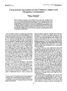
1 Introduction Two illuminated surfaces of different reflectance can appear to have their colors bleed into one another in regions where light reflected from one surface falls onto the other surface. This is a mutual reflection effect. Figure 1 shows two surfaces that form an edge, and the resulting interreflection effect. In this article we examine how the lights reflected separately from each surface combine to form RGB values in the mutual reflection region. Using vector models for the illumination spectral power distribution and for surface reflectance functions we show that by looking at the extra information coming from measurements of the interreflection RGB values--in addition to sensor measurements from each surface separately--it is possible to recover the surface reflectance properties of both surfaces. In this way we use mutual reflection to obtain "color constancy." The term color constancy refers to the ability of humans and some animals to perceive object colors as approximately constant, independent of changing illumination (see, e.g., Beck 1972). There is evidence that several simultaneous mechanisms contribute to color constancy in humans (Blackwell & Buchsbaum 1988).

Nevertheless, we have found in (Ho, et al., 1990), that it is the case that an algorithm can be built to recover reflectance from the color signal, in which illumination and surface characteristics are confounded, without regard to colored surrounds, selective adaptation, memory of colors, etc., provided that the complete color signal is known. Most recent attempts to accomplish this end have made use of finite dimensional linear models in which illumination and surface spectral reflectance are approximated by a weighted sum of a few basis functions of wavelength (Brainard et al. 1989; Brill & West 1986; Buchsbaum 1980; D'Zmura & Lennie 1986; Gershon et al. 1987; Maloney 1985; Maloney & Wandell 1986; Wandell 1987; Yuille 1987). In the innovative work of Maloney and Wandell 1985; 1986; 1987, several special conditions have to be true for reflectance to be recoverable from the color signal entering the camera. Some of these conditions are that the illumination must be constant over a given segment of the image, and that a sufficiency of different color information must be available over the image. More importantly, in this method the number of sensor classes (e.g., 3 for RGB sensors) must be at least as great as the number of basis functions modeling the surface spectral reflectance, plus 1. This means that for a usable

6

Funt, Drew and Ho

/ /

1

X

E tx~

E C~)

E (~)

I

(~.) A

S (i)(~) s" J

J ,s

J

s"

,t

f

S 121(;~) 2 Fig. 1. Isotropic illumination with spectral power distribution E(k) impinges on surfaces 1 and 2, which have surface reflectance functions S(])(k) and S{2)(k) respectively. Far from the edge, surface 1 reflects color signal I (1}(k) toward the camera; and, similarly, surface 2 reflects (2} l (k). Close to the edge, E(k) is augmented by light reflected from the other surface. The color signals reflected from the surfaces near

the edge are l~)(k) and l~)(k). dimensionality for the set of basis functions modeling reflectance, say 3 or better (Maloney 1986), one must somehow develop a "fourth sensor class" to provide enough information to allow a solution that disentangles illumination and surface spectral reflectance. Alternatively, one can continue using the usual 3 sensor classes, but at the expense of having only a dimensionality of 2 with which to model surface reflectance. Maloney and Wandell's method essentially involves writing down a set of equations relating the sensor values Ok, k = 1 . . . p , to the finite dimensional linear

model weights, Ei, i = 1 . . . m for illumination, and crj, j = 1 . . . n for surfaces, and then coupling the sets of equations at different pixels by using the assumption of constant illumination. Taking into account enough pixels, which must have sufficiently different sensor values, brings the number of equations equal to the overall number of unknowns, allowing a solution for e, and aj. In Ho et al. (1990) it was shown that the need for additional sensor values can essentially be fulfilled by requiring that a finer sampling of the color signal

Color Constancy from Mutual Reflection spectrum be introduced as additional input. In that work, it was shown that from detailed knowledge of the spectral power distribution of the color signal, a complete disambiguation of the reflectance and illumination from the color signal is possible, and in fact is possible independently at each pixel and without the need for constant illumination or any special requirement on the richness of color variation over image segments. This method (Ho et al. 1990) relies on a statistical determination of the finite dimensional model weights using a least-squares method, and has the sole requirement that a special mathematical relationship holds among the basis vectors, viz. that the set of functions generated by forming products of the basis functions for illumination and surface reflectance forms a linearly independent set. The main benefit of this method is that one can increase the dimensionality of the surface reflectance space without having to increase the number of Ok values beyond the 3 that correspond to the cones in the human visual system. In Funt & Ho (1989) and Gershon et al. (1986, 1987) it was shown that the required spectral information for the color signal is derivable from the chromatic aberration effect at edges between adjacent color regions. In fact, what is found via chromatic aberration is the difference between color signals from each side of the edge. Coupled with the method of Ho et al. (1990) and given this spectral information plus RGB sensor values from each side of the edge, the values of ei and oj can be determined and color constancy achieved. In this article, we take a different approach, although the basic motivation is the same--we seek more information than just the Pk values in order to circumvent the "fourth sensor problem." Here, we consider the mutual reflection at a 3-dimensional edge, and the resulting bleeding of colors at the 2-dimensional image edge, without regard to chromatic aberration. Such interreflections generally occur near the edges of objects and the boundaries where objects occlude one another (Horn 1986). We can take measurements of Pk values from pixels where mutual reflection effects are present and compare them to values where such effects must be absent or small. By using such measurements on each side of an image edge, relatively far from the edge and also relatively close to the edge, we capture sufficient information to determine ~i and 0rj separately on each side of the edge, and hence determine the true reflectance for each color patch. This is more than enough information to provide color constancy. In Gershon et

7

al. (1986) it was shown that mutual reflection can help to distinguish shadow boundaries from material changes. Here we show that mutual reflection has another positive aspect--it is an effect that can be exploited to achieve color constancy. As well, once constant color descriptors are found, the mutual reflection component can be effectively removed from the image. Such an image filter could be useful for shape-fromshading, etc. (Forsyth & Zisserman 1989, 1990). The only constraint on the formulation turns out to be that the numberp of sensor classes must be greater than or equal to (2n + m)/3, where m and n are the number of basis functions required to model illumination and surface spectral reflectance respectively. This constraint is satisfied by values p = m = n = 3 and hence we can keep to only 3 sensor classes while still allowing n = 3 for describing reflectances. These values of p, m, and n are shown to recover both surface spectral reflectance and illumination spectral curves well within acceptable errors. Here, we address only a small part of a large problem. We assume a preliminary edge-finding and segmentation algorithm that would identify those edges where mutual reflection might be present. Given such identification of appropriate sites our analysis concentrates on extracting any available reflectance information from mutual reflection effects. In section 2 we show how p, measurements on each side of a color edge, and inside the mutual reflection region, are related to the values of ei and aj for each side of the edge separately, assuming a finite dimensional linear model for describing natural lighting and reflectances. The resulting model is quite complex, but some reasonable assumptions reduce the equations to solvable form. We show that a reciprocity relation exists between the mutual reflection measurements on each side of an edge, so that only Pk values in the mutual reflection zone on a single side of the edge are required. In section 3 an algorithm is presented for solving for the reflectance weights aj on each side of the edge separately, as well as the illumination weights ei, which are assumed to not change across an edge. We develop a uniqueness proof that guarantees convergence of the algorithm. In section 4 we set out the geometrical significance of the mutual reflection configuration factor used in the analysis. In section 5 we examine the accuracy of the solution method by carrying out simulations. The results are

8

Funt, Drew and Ho

seen to be very good in most cases, with accuracies of the resulting reflectance spectra not degraded much from the accuracy of the underlying finite dimensional model.

2 Finite-dimensional Models Applied to Mutual Reflection 2.1 Mutual Reflection Equations We assume that illumination and surface spectral reflectance are each modeled to an acceptable degree of accuracy by finite dimensional linear models. Depending on the dimensionality of the set of basis functions, not all illumination spectra and surface reflectances will be well modeled; generally, the higher the dimensionality of the set of basis functions the better will be the approximation (see, e.g., Maloney 1986). However, we shall show below using simulations that whether or not the accuracy of the underlying finite dimensional model is good, the accuracy of the solution for color constancy from mutual reflection measurements is not greatly reduced. For reflectance basis functions we use those determined by Cohen via a statistical principal component analysis of 150 Munsell chips randomly selected from a total of 433 chips (Cohen 1964); see also Parkkinen et al. (1989). For illumination, a similar analysis was carried out by Judd et al. (1964) for 622 typical daylight samples. We demonstrate below that it is possible to use n = m = 3 basis functions for surfaces and illumination and still have only p = 3 sensor classes. Most naturally occurring daylights and many surface reflectances can be approximated reasonably well using these basis functions, so that by determining a good approximation of the weights ei and aj, we are in fact deriving an approximation of the entire illumination or reflectance spectrum. Hence what we require from a solution is actually more stringent than simply color constancy, in that we seek to recover more information than just chromaticity values. And, in fact, the measure of accuracy we shall use is the error sum of squares over the entire visible spectrum of an approximate reflectance spectrum compared with an actual one. Consider the situation depicted in figure 1. lsotropic illumination E(X), assumed constant across an edge, impinges on two surfaces, 1 and 2. Assume surface 1 has spectral reflectance function S0)(X) and surface 2

has reflectance S(2)(X), all surfaces being ideal diffuse (i.e., Lambertian) reflectors. Then depending on the geometry, interreflection may be present as shown in figure 1. In fact, the two surfaces need not meet at an edge for a mutual reflection effect to come into play; and we do not require the surfaces to be flat. We show ray geometry in figure 1 to clarify the interreflection process. However, ray geometry is actually unnecessary since perfect diffuse reflectors obliterate directional information: reflections are really in all directions into the hemisphere above each surface. We assume here that illumination is uniform on each surface and hence exclude shadow situations. Expanding the illumination function in terms of m basis functions, the spectral power distribution can be approximated by the sum

E(X)

= ~] eiEi(~,) i=1

with weights el. Similarly, for surface 1 the reflectance can be written

s(°(x) = ~] o}')s,(x) j=l

where reflectance is modeled by n basis functions with n weights o}t). Surface 2 has reflectance

S(2)(X)

~ (2)S0k) j=l

The color signal I(X) is the light reflected by the surface, and is given by the product of E and S. On the surface 1 side, at a point relatively far from the edge, the color signal is simply IO)(X) = E(X) SO)(X) Similarly, on the surface 2 side we have I~2)(X) = E(X) Sa)(X) Substituting the basis function decomposition, we have

i=lj=l

i=l j=l

Color Constancy from Mutual Reflection NOW consider the mutual reflection region in which part of l(1)(~k), the light reflected from surface 1, impinges onto surface 2. Similarly, part of I(2)(X) impinges onto surface 1. The amount of l(l)(~k) that is intercepted by surface 2 is dependent on both the configuration of the surfaces and on the shape of each surface, since not every reflected ray is intercepted (consider a small triangle of surface 1 forming an edge with a large plane of surface 2). In computer graphics diffuse interreflections are modeled using configuration factors that give the fraction of light from one surface that reaches another surface (Goral et al. 1984). We discuss these in section 4. Since there is no a priori reason to assume that one surface is more reflective than the other (although for clarity in figure 1 only a single interreflection is shown), we consider the fraction ~x~2of I(X) from 1 that strikes 2, and the similarly defined ~xz~. Denote by I ~ ) the color signal from a spot on surface 2 in the mutual reflection region, so that it includes a contribution from light reflected by surface 1. It consists of two parts. The first part is I(2)(X), the reflection of E(X) from surface 2. This we assume is the same as from a spot relatively far from the edge, outside the mutual reflection region. The second part is due to the light reflected from surface 1. Since the latter is presumed to come from a spot on surface 1 that is near the edge, the second part is a contribution from I~ ) (cf., Goral 1984). Hence the color signals coming from each side of the edge in the mutual reflection region are

9

2.2 Simplified Equations The above set of equations would be quite difficult to solve numerically. However, since both c~ and S(X) are less than 1, in most cases not much accuracy is lost by rewriting the equations to first order in a • S. This amounts to ignoring more than one bounce of the color signal between the surfaces. With typical values of S 0.01-0.3 and typical values of a of _ m + 2n + 1 holds. Therefore we cannot use p = m = n = 3 unless we impose a further constraint. Since we must only expect solutions to yield illumination and surface reflectance spectra up to a multiplicative constant, because the ei and oj occur in products in the color signal, we must make one further requirement on one of the ~i o r O'j; we choose to set el = 1. That is, for surfaces we determine reflectance but not brightness.

O'J1),

11

Now our condition reads p _> (m + 2n)/3 and we have a nonlinear set of equations for ci, o)1), o)2), and c¢ that is at least sufficient for a solution. Since the set of equations is also clearly independent, in that one cannot write any equation in terms of the others, we would be confident of having fulfilled necessary and sufficient conditions for a solution if the set of equations were linear; however, because they are nonlinear we must proceed with caution.

3 Implementation and Results We reduce the solution of the nonlienar set of equations (3), (4), and (5) to the solution of linear ones by breaking up the solution into a multi-stage algorithm. Starting with some reasonable initialization for el, we iteratively solve in turn for o)1), then o}2), and finally el. The condition ~l - 1 at each step of the iteration also forces a to converge. In detail, with respect to equations (3), (4), and (5), we use the following algorithm: Initialize e~ = ~2 = e3 = 1 Step 1: Use (3) to solve for o)l) in terms ofei, since (3) is linear in these unknowns Step 2: Use (5) to solve for a • a) 2) in terms of ei and o)j). Step 3: Use (4) to solve for ej + ~ in terms of O~ • O'J 2) .

S t e p 4 : Now setel =- 1: i.e., setel + c~ ~ 1/a. Therefore, set c~ *- 1/el and ei ~- ei/~l. Iterate until all values in the set {~i, a) 1), oj(2), a} change less than a prescribed tolerance, Since the equations are nonlinear, the order of the above steps is important. We found by trial and error that the steps in the order described lead in a stable fashion to the desired solution. The algorithm produced stable, unique results regardless of how the initial values for ei were chosen over a wide range. However, for the first initial value we imposed the constraint E1 -- 1 from the outset. We also found that when the underlying finite-dimensional model did an extremely poor job of describing both surfaces, the algorithm was slow to converge and did not do as well in recovering surface reflectance. We explore this situation in section 5 by looking at very noisy, poorly modeled surfaces. An important consideration is that the algorithm should obtain a unique solution. Uniqueness and speed of convergence can be established by converting the

12

Funt, Drew and Ho

problem to be solved into the form of a fixed-point problem (see, Burden et al. 1981). Choosing a particular algorithm corresponds to adopting a particular fixedpoint version of a problem. There are often several possible options, and not all of them converge. We can investigate the convergence properties of our algorithm by explicitly converting it to the fixed-point form to which it is equivalent. Then the well-known contraction mapping theorem can be used to test uniqueness as well as give rates of convergence. Following Steps 1, 2, and 3, we algebraically solve for functions o) = ~ (1)(~., ~ o))

(6)

(2) = ~ (:)(a, ~, ~(1), ~)

(7)

where

____~m(2)_ ~(2) and finally

---- e(o/, ~, p (1), ~, ~ (2))

(8)

where we denote by ~ the solution of equation (4) for ~'. Now since we set e~ - 1, we can solve the 6~ component of equation (8) for a, so that a is given in terms of 62, 63, and the camera RGB values ~, only. Substituting this value of t~ into the remaining equations for 62 and 63 gives a set of two equations in fixed-point form:

62 = e2(62, 63, RGB)

(9)

63 = e3(62, 63, RGB) where we have denoted the set of observed camera RGB values simply as RGB. To prove uniqueness we must show (a) that when the values of 62, 63 are allowed to range over a reasonable domain D, then the right-hand sides of equations (9) will also be confined to D; and (b) that the absolute values of all possible first partial derivatives of the two right-hand sides with respect to 62, 63 are bounded by a constant K/2 with K < 1. When conditions (a) and (b) are satisfied, the vector function [e2(62, 63, RBG), e3(62, 63, RGB)] is guaranteed to intersect with the vector function [e2, e3] -- [62, 63] at a single point. These conditions also prove convergence of the sequence provided by the algorithm, with the rate of convergence being controlled by the bound of the derivatives. What this uniqueness check amounts to is carrying out the first iteration of our algorithm over a large domain D of initial values of 62, 63 and examining the resulting solution values e2, e3 after a first pass. If the

values of e2, e3 are within the search space of initial values c2, 63 and if the partial derivatives of 62, e3 with respect to both 62 and 63 are everywhere sufficiently small, then the algorithm is guaranteed to converge to a unique solution. Since the first-pass estimates e2, e3 of 62, 63 are generated using the particular observed sensor values ~(l), ~, ~(2) corresponding to the pixels under examination, we cannot make a blanket statement of uniqueness for our algorithm. There may be cases in which one cannot prove the theorem guaranteeing unique convergence, even when such cases do in fact converge correctly. We implemented the uniqueness check as a preprocessing algorithm for the equation-solving algorithm. For a particular input set of sensor values, it is straightforward to search a wide domain of initial values of 62, 63 and take partial derivatives of the firstpass estimates 62, e 3. We found in our simulations (section 5) that uniqueness was guaranteed except in those cases where the finite dimensional model itself represented the surfaces very poorly. Thus the preprocessing step is a useful filter for screening out any pixels for which the algorithm may not converge, such pixels generally corresponding to surface reflectances poorly captured by the finite dimensional model. In the equation-solving algorithm itself, it is importaut to note the way in which a appears. Since it always appears in combination with another variable until the final normalizing step, the only place where the above algorithm's accuracy of solution for ~ and for all the variables is affected by the particular value of cz is in forming I~)(X) in equation (2). As a result, the accuracy of solutions depends only very weakly on the particular value of a. We found (see simulations in section 5) that a change of ct from 0.01 to 0.5 resulted in only a 6.7 % change in the accuracy of the solution for ~, with similar results for the other variables. So long as the mutual reflection effect is indeed present, the solution proceeds to find t~. No matter what the actual value of c~ the percent error in tx will be nearly constant for a particular illumination and set of reflectances for the two surfaces. As well, the accuracy of the reflectances recovered depends only weakly on the particular value of a dictated by geometry. Of course, this near-independence with respect to a is true mathematically but noise will break this situation down somewhat. We investigate below the effect of noise on the solution. As well, as c~ ~ 0 we expect the method to fail; this would correspond to the case of negligible interreflection.

Color Constancy from Mutual Reflection

13

In section 5 we apply the algorithm to several cases involving synthesized color signals composed from naturally occurring lights and reflectances. In the next section we investigate the geometrical significance of the factor o~.

4 Configuration Factors One may ask whether in general there will exist points on a surface where we can effectively say that no mutual reflection effect exists. We can answer this question by examining the structure of the parameters a12 and a21. The total irradiance onto surface B from surface A as a fraction of the total radiance emanating from surface B into the hemisphere above it is termed the form-factor in illumination engineering. Here we are interested instead in how much light reflected from one surface is intercepted at a particular spot on the second surface. A catalog of such configuration factors (total irradiance as a function of position on surface B incident from all points on surface A) has been assembled by Siegel and Howell (1981). In general, configuration factors can be calculated for any geometry and are independent of wavelength for ideal diffuse reflectors. For illustrative purposes, consider for simplicity a relatively long (effectively semi-infinite) planar edge (figure 2). Let the fraction of light from the small area AAI intercepted by the upper surface Az, divided by the total amount of light from AAI into the hemisphere above it, be F12. Calculation of the quantity Ft2 will effectively yield the fraction of light F2, from A2 intercepted by AA1 as well, because of the reciprocity relation for configuration factors (Siegel & Howell 1981).

A2F21 = AAIF12 If I(k) is measured in W/m 2 of unprojected area then the power in a wavelength interval received over A2 from light I

0.8

1000 -

__a 03

900 -

-0.6 .~x ©

(3

~.~

,--

(..)

E

800 -

C,O

0

-0.4 ~cD re"

700 0

(,3 600 .0

0.2

-4--

(3

.___

500

-

E 4 0 0 4 3 0 460 490 520 550 5 8 0 610 6 4 0

Wavelength

(nm)

Fig. 5. Typical case: color signal formed from product of surface spectral reflectance Krinov #54 and Dixon spectrum for Australian daylight. The color signal has been scaled up by a factor of 6.

in developing a principal-component analysis for Australian daylight, but here we truncate to the visible, 400 nm-650 nm. The spectrum for the mean vector for daylight in Bendigo, Australia, is shown in figure 5 along with Krinov reflectance curve #54 and the resulting color signal composed of the product of the two spectra. For the domain D of initial value c2, c~s to use in the uniqueness check preprocessing step we took the largest absolute values of e2 and e3 for all of Judd's curves and then doubled that region. We suppose for simplicity that the shape and geometry of the two surfaces leads to geometrical factors of ~21 (]{12 -- C¢ = 0.05 for mutual reflection. The algorithm of section 3 applied to the two color signals generated from this illumination spectrum and Krinov reflectances #53 and #54 can be tested by forming sensor values pit), piE), and p~. To develop these signals, we used sensitivity functions (see figure 6) corresponding to Kodak filters #25 (red), #58 (green), and #47B (blue). The algorithm results are quite good: the =

value of a found by the solution method is 0.0495, so that the ratio of the estimated t~ to the actual one is 0.990. As pointed out above, using the approximate model algorithm the accuracy for this ratio remains nearly constant no matter what the actual value of c~ is. To develop an error figure for the spectral reflectance function, it is important to recall that the algorithm gives a solution only up to an overall multiplicative constant. Therefore, the shape of the reflectance curve is derived, but not its absolute scale. To make a fair comparison, we scale by an appropriate factor and then calculate the error statistic. A best match of the derived curve and the actual one is found by solving for the multiplicative factor by minimizing the squared residuals after multiplying by the unknown factor. The normal equation for this minimization problem yields the factor. As shown in figure 7, the spectral curve for reflectance 2 is quite close to that for Krinov #54; the overall error for the curve found by our algorithm is 9.71%.

Color Constancy from Mutual

Reflection

17

10

Red 8

Green Blue

-t--

.> 6 r-

>

°~ -t,,,-

; I

4-

cJ

I

/\,

ct/ 2-

0

\

:

\/

ixxJ,,, t

i

I,

I

J"

t

t

r

t

400430 460 490 s20 550 sao 610 640

Wavelength (nm)

Fig, 6 Kodak filters #25 (red), #58 (green), and #47B (blue).

Since the error of the best fit using the underlying finite dimensional model is 8.11%, the ratio of our model error to the finite dimensional model error is only 1.197. The fit for surface 1, which has reflectance Krinov #53, is similar. We show in figure 8 the results of the algorithm in recovering the illumination compared to the actual spectrum. Again, the increase in error is quite small--we obtain an error of 4.10% as compared to the finite dimensional model error of 3.97%. In table 1, we show the results of running the algorithm on sensor values derived from the same reflectances as above for all five of Judd's standard daylights, corresponding to five different correlated color temperatures, as well as the Dixon spectrum. As can be seen, the results are similar for all illuminations.

As well, uniqueness was validated by the preprocessing step in these cases. A more stringent test is carried out by utilizing atypical reflectance curves that are not well modeled by the basis functions. For this test we use Krinov #162 ("grass, young, green") along with Krinov #54. A best fit using the finite dimensional model itself has an error of 26.65% for Krinov #162. The results for the algorithm are again reasonably good, as seen in table 2. To take into account noise, we add a random perturbation to each p-vector separately; each component independently receives additive noise equal to a percentage of the vector magnitude. For this test we use the Dixon spectrum coupled to reflectances Krinov #53 and Krinov #54. Running the algorithm repeatedly, we

18

Funt, Drew and Ho

0.20/

0.161

L..

¢0 E 0

0.12

"

"

"/ ~

i

•

~

'6

0.08

Actual

0.04

A..~.£~h..rnr.e..s r u~! Best fit

0.00

I

I

I

I

I

I

I

I

400430 460 490 520 550 580 610 640

Wavelength(nm)

Fig. 7. Comparison of the best fit given by dimension-3 finite dimensional model with surface spectral curve resulting from the algorithm. The best-fit error (here, the reflectance curve is Krinov #54) has error = 8.11%, whereas the algorithm result has error = 9.71%, a factor of 1,197 worse than the best fit. When the geometrical mutual reflection factor a is 0.05, the algorithm gives the value 0.04949, so that the ratio of the estimate to the actual a is 0.9898.

arrive at average results, shown in table 3. Here, the 0% noise case is shown for comparison and all other figures are averages. For a few very poorly fit noisy signals at the higher noise level, the algorithm is less stable and a greater tolerance must be used for halting iteration. For each of these cases the uniqueness check also showed that the results were unreliable. So for a large noise component the results are not good. Nevertheless, the results are reasonably good for low noise, and in that regime the stability of the algorithm is very good. The number of iterations through the algorithm was typically 6 to 8. If use is made in our model of broad-band sensor

functions such as those in the human visual system, instead of bandpass filters common in video and film, then the results of the algorithm are found to be somewhat more accurate since a broader sampling of more frequencies results in a better representation of the entire color signal spectrum in terms of the finite dimensional model weights.

5.2 Infinite-zone Edge In Drew and Funt (1990), we simulated the full physics (infinite-zone, infinite-bounce) of the interreflection at

Color Constancy from Mutual Reflection

19

1200

1100

i

~

.

1000 ._c 900

'

> ° ~

800 E

._o (3 E

E

700 600 Actual 500

Algorithm result Best fit

400

I i I J I I ] I 400430 460 490 520 550 580 610 640

Wavelength (nm)

Fig. 8. The original Dixon illumination spectrum for Australian daylight and results of the mutual reflection algorithm applied to the color signal of figure 5--error 4.10%.

an edge under diffuse illumination by employing the radiosity method (Goral et al. 1984). However, unlike the usual approach in computer graphics, we carried out the radiosity calculation separately on each wavelength instead of on the usual three color bands and therefore could not use standard computer graphics radiosity tools to synthesize test images. In generating a correct color distribution at the edge it is crucial that one apply the filter functions to generate RGB values only after calculating the entire color signal spectrum for each pixel. We used this method on the edge of figure 2, using Krinov spectra #54 and #248 and incident illumination D65. Figure 9 shows the variation in RGB on surface 2 that occurs with increasing distance from the edge. For comparison, the (constant) RGB values resulting

from S(2)(~)E(X) in the absence of interreflection are also plotted. The ratios R/B and G/B graphed in figure 10 show that not only the intensities, but the colors too change with distance from the edge. We can see from figure 10 that derivatives of ratios approach zero as one gets farther from the edge. Running our mutual reflection analysis algorithm on the calculated RGB image data, we find that reflectances on each side are recovered quite accurately. Except at pixels very close to the edge, the algorithm obtains a reflectance S(2)(X) that is virtually independent of position. The error with respect to the actual reflectance spectrum is 4.37%, which translates into a color difference AE of 3.54 units in CIELUV uniform color space (see Wyszecki and Stiles 1982). For surface 2, the best least-squares approximation using the finite

20

Funt, D r e w and H o

Table L Errors using typical reflectances: Krinov #53 and #54, t~ = 0.5, and Judd's North American daylights of five different correlated color temperatures as well as Dixon's Australian daylight. The finite dimensional model best curves have errors of 11.04% for Krinov #53 and 8.11% for Krinov #54. Columns show: (1) ct recovered by algorithm; (2) ratio of the recovered c~to the actual one; (3) error for illumination spectrum found by algorithm; (4) absolute error of reflectance curve found by algorithm for surface 1; (5) error of reflectance curve for surface 1 compared to error in underlying finite dimensional model; (6, 7) similarly for reflectance curve for surface 2. For the Dixon case, the finite dimensional model illumination modeling error is 3.97%, so that the ratio E(~,) Error / E(X) ErrorFD M is 1.032. Daylight

c~

neST

E(X)

R~I)(X)

R0~(X) Error

Rt2)(M

R~z/(~,) Error

aACT

Error (%)

Error (%)

R~I~(X) ErrOrFDM

Error (%)

R~2~(X) ErrorFoM

4800K

0,04971

0.9943

0.30

11,35

1.028

9.81

1,209

5500K

0.04971

0.9942

0.29

I 1.34

1.027

9.79

1.206

6500K

0.04973

0.9945

0.31

11.34

1.027

9.75

1.202

7500K

0.04972

0.9944

0.31

11.32

1.026

9.73

1_200

10000K

0.04972

0.9944

0.31

11.33

1,026

9.70

1.196

Dixon

0.04949

0.9898

4.10

11 3 4

1.027

9,71

1,197

Table 2. Poorly fit case: reflectances Krinov #162 and #54, c¢ = 0.05--errors for five Judd daylights and for Dixon daylight (best model fit has error 26,65% for Krinov #162 and 8.11% for Krinov #54); ~ recovered by algorithm; compared to correct oL; illumination spectrum error found by algorithm; reflectance curve 1 error; compared to error in underlying finite dimensional model; similarly for reflectance curve 2. For the Dixon case, the finite dimensional model illumination modeling error is 3.97%, so that the ratio E(X) Error / E(X) ErrorFD M is 1.428. Daylight

a

OteST

E(X)

R(I)(X)

R0)(),) Error

R(2)(X)

R(2)(X) Error

OtACT

Error (%)

Error (%)

R0)(~,) ErrOrFDM

Error (%)

R(2)(X) ErrorFoM

4800K

0.04988

0.9975

3_47

32.29

1.212

11,13

1.371

5500K

0,04987

0.9974

3.41

32. I 1

1.205

l 1.04

1.361

6500K

0.04988

0.9976

3.37

31.93

1.198

10.95

1.349

7500K

0,04987

0.9974

3.19

31.83

1.194

10.89

1.342

10000K

0,04987

0.9974

2.86

31.68

1.189

10.80

1.331

Dixon

0.04964

0.9929

5.66

31.95

1.199

10.90

1.343

Table 3. Noise: reflectances Krinov #53 and #54, Dixon spectrum, o¢ = 0.05--finite dimensional model best fits have E(X) ErrorFD M = 3,97%, R0)(K) ErrorFD M = 11.04%, and R(2)(),) ErrorFD M = 8. I 1%. Columns show: t~ recovered by algorithm; compared to correct c~; illumination spectrum error found by algorithm; reflectance curve 1 error; reflectance curve 2 error.

OtEST Noise (%)

ce

'

t~ACT

E0Q

R(I)(h)

R(2)(•)

Error (%)

Error (%)

Error (%)

0

0.04983

0.9967

4.13

11.33

9.75

5

0.04385

0.8771

17,13

16.80

15.05

10

0.03912

0.7823

38.50

29.030

28.34

Color Constancyfrom Mutual Reflection

21

0.23

_

m

m

13 E

Red 0.20

rn

Green Blue

C~

0.17

Distance from edge

Fig. 9. RGB variation on one side of an edge due to mutual reflection.

dimensional model with dimensionality 3 gives an error o f A E = 3.25; clearly, the mutual reflection method contributes only a small additional error. For illumination, the error of the recovered spectrum is virtually zero. The recovered values of t~ vary as shown in figure 11. Here we have scaled c~ to take into account the scaling of the illumination E that gives e~ = 1. For comparison we also show the theoretical configuration factor ~ as determined by equation (10). We display that factor offset so that it goes to zero and not to the small value it takes on at the pixel farthest from the edge. As one would expect since the recovered ~ maps the contributions from all bounces into a one-bounce factor, it is marginally larger than the theoretical ct generated using equation (10) that models an infinitezone, one-bounce situation.

6 Conclusions We have examined the effects of mutual reflection in color images. Since mutual reflection causes the spectrum of the light reflected from a surface to vary with location on the surface even though the surface reflectance is constant, it provides clues to the actual surface reflectance and to the geometry of the situation. Tests show that the algorithm is quite robust. The method has the potential for eliminating mutual reflection effects and in most cases recovers a good approximation of the complete spectral information. Thus the method yields more than enough information to supply color descriptors for the object surfaces that are independent of ambient illumination; therefore, color constancy is obtained. Sensor values from only three

22

Funt, Drew and Ho

0.885

0.863

I\ ,

c 0

0.861

X

R~ RIB

0 >

o o o

0.859 -

0.857 -

0.855

Distance from edge

Fig. 10. Color variation: ratios of R/B and G/B for figure 9.

pixels need to be measured to obtain a result and the method will work on surfaces that do not meet the surface complexity conditions needed to make Maloney and Wandell's algorithm work. The elimination of mutual reflection is a desirable feature in a vision system since it is an effect that introduces extra complexities; that is, it is known to create problems in shape-from-shading schemes (Forsyth & Zisserman 1989, 1990). Clearly, the interreflection model put forward here, that uses basis function decompositions for an accurate whole-spectrum model of reflection, can be extended to the modeling of multisurface enclosures for graphics applications (cf. Goral et al. 1984). Multiple interreflections could be incorporated at the expense of having a more difficult mathematical system to solve; for

enclosures, such multiple bounces may add a significant contribution. Ignoring multiple bounces for 3, 4, etc., surfaces results in a simple set of linear equations similar to the linear equations for Im(k) in section 2. The algorithm still works even if both surfaces have the same color, with the same or differing brightness. This case might correspond to a folded piece of uniform material. The recovery of c~ here gives shape information near the fold. The method works in this one-color case because the reflected light is a different color from the illumination, and the extra measurements of sensor values supply enough information to disentangle the two.

The results show that, in situations in which mutual reflection is present, measurements of the sensor values taken separately from the two different interreflecting

Color Constancy from M u t u a l Reflection

23

0.5

0.4

~3 L O (O [3

Theoretical factor, offset to zero 0.3

Recovered a, scaled

E O , m ~D L.

O3

° _

0.2

E O C)

0.1

0,0

Distance from edge

Fig. 1l. Variation of one-bounce, two-zone ~ factor, where the sensor RGB inputs are derived from a full multi-zone model. Theoretical onebounce, infinite-zone factor is shown for comparison. surfaces, as well as f r o m within the mutual reflection zone, can convey sufficient information to allow c o m plete recovery of the two surface spectral reflectance functions as well as of ambient illumination. We also recover the factor ~, w h i c h s u m m a r i z e s information about the relative g e o m e t r y of the two surfaces.

7 Acknowledgments M.S. D r e w is indebted to the C e n t r e for Science at S i m o n Fraser University for partial B.V. Funt thanks both the CSS and the Natural and E n g i n e e r i n g Research Council of C a n a d a support.

Systems support; Sciences for their

References Beck, J. 1972. Surface Color Perception, Cornell Univ. Press: Ithaca, N.Y. Blackwell, K.T., and Buchsbaum, G. 1988. Quantitative studies of color constancy. J. Opt. Soc. Amer. A., 5:1772-1780. Brainard, D.A., Wandell, B.A., and Cowan, W.B. 1989. Black light: How sensors filter spectral variation of the illuminant. IEEE Trans. Biomed. Eng. 36:140-149, 572. Brill, M.H., and West, G. 1986. Chromatic adaptation and color constancy: A possible dichotomy. Col. Res. Appl. 11:196-204. Buchsbaum, G. 1980. A spatial processor model for object colour perception. J. Franklin Inst. 310:1-26. Burden, R.L., Faires, J.D. and Reynolds, A.C. 1981. Numerical Analysis. Prindle, Weber & Schmidt: Boston. Cohen, J. 1964. Dependency of the spectral reflectance curves of the Munsell color chips. Psychon. Sci. Amer. A. 6:318-322.

24

Funt, D r e w a n d H o

Dixon, E.R. 1978. Spectral distribution of Australian daylight. J. Opt. Soc. Amer. 68:437-450. Drew, M.S., and Funt, B.V. 1990. Calculating surface reflectance using a single-bounce model of mutual reflection. Proc. Intern. Conf. Comput. Vision, Osaka, December 4-7. D'Zmura, M. and Lennie, E Mechanisms of color constancy. J. Opt. Soc. Amer. (10):1662-1672. Forsyth, D., and Zisserman, A. 1989. Mutual illumination. Proc. conf. Comput. Vision Patt. Recog., San Diego, pp. 466-473. Forsyth, D., and Zisserman, A. 1990. Shape from shading in the light of mutual illumination. Image Vision Comput. 8:42-49. Funt, B.V., and Ho, J. 1988. Color from black and white. Proc. 2nd Intern. Conf. Comput. Vision, pp. 2-8, Dec. 5-8, Tarpon Springs, FL. Funt, B.V., and Ho, J. 1989. Color from black and white. Intern. J. Comput. Vision 3(2). Gershon, R., Jepson, A.D, and Tsotsos, J.K. 1986. Ambient illumination and the determination of material changes. £ Opt. Soc. Amer 3: r/00-1707. Gershon, R., Jepson, A.D. and Tsotsos, J.K. 1987. From [R,G,B] to surface reflectance: Computing color constant descriptors in images. Proc. lOth IJCAI, Milan, pp. 755-758. Goral, C.M., Torrance, K.E., Greenberg, D.E and Battaile, B. 1984. Modeling the interaction of light between diffuse surfaces. Computer Graphics 18:213-222. Ho, J., Funt, B.V., and Drew, M S . 1990. Separating a color signal into illumination and surface reflectance components: Theory and applications. IEEE Trans. Patt. Anal. Mach. Intell. 12:966-977. Horn, B.K.E 197Z Understanding image intensities. Artificial Intelligence 8:201-231. Horn, B.K.E. 1986. Robot Vision. MIT Press: Cambridge, MA. Judd, D.B., MacAdam, D.L., and V~szecki, G. 1964. Spectral distribution of typical daylight as a function of correlated color temperature. J. Opt. Soc. Amer. 54:1031-1040, August.

Krinov, E.L. 1947. Spectral reflectance properties of natural formations. Technical Translation TT-439, National Research Council of Canada. Koenderink, J.J., and van Doom, A.J. 1983. Geometrical modes as a general method to treat diffuse interreflections in radiometry. J. Opt. Soc. Amer. 73:843-850. Maloney, L.T. 1985. Computational approaches to color constancy, Ph.D. dissertation, Stanford University, Applied Psychology Laboratory. Maloney, L.T. 1986. Evaluation of linear models of surface spectral reflectance with small numbers of parameters. J. Opt. Soc. Amer. A, 3:1673-1683. Maloney, L.T., and Wandell, B.A. 1986. Color constancy: a method for recovering surface spectral reflectance. J. Opt. Soc. Amer. A, 3:29-33. Nayar, S.K., Ikeuchi, K., and Kanade, T. 1990. Shape from interreflections. Proc. Intern. Conf. Comput. Vision, Osaka, December 4-7. Parkkinen, J.P.S., Hallikainen, J., and Jaaskelainen, T. 1989. Characteristic spectra of Munsell colors. J. Opt. Soc. Amer. A, 6:318-322. Siegel, R., and Howell, J.R. 1981. Thermal Radiation Heat Transfer. Hemisphere Publishing Corp: New York. Sparrow, E.M., and Cess, R.D. 1978. Thermal Radiation Heat Transfer. Hemisphere Publishing Corp.: New York. Wandell, B.A. 1987. The synthesis and analysis of color images. IEEE Trans. Patt. Anal. Mach. lntell. 9:2-13. Wyszecki, G_, and Stiles, W.S. 1982. Color Science: Concepts and Methods, Quantitative Data and Formulas. Wiley: New York. Yuille, A. 1987. A method for computing spectral reflectance. Biological Cybernetics 56:195-201.