to help choosing a color space and to generalize the correlation measures to color. .... arccos H1 if B ⤠G. 2Ï â arccos H1 otherwise. H1 = (RâG)+(RâB). 2â.
COLOR CORRELATION-BASED MATCHING S. Chambon∗ and A. Crouzil∗
Nine color spaces are evaluated and three methods are proposed: to compute the correlation with each color component and then to merge the results; to process a principal component analysis and then to compute the correlation with the first principal component; to compute the correlation directly with colors. Moreover, an evaluation protocol which enables to study the behavior of each method with each color space is required to highlight the best way to adapt correlation measures to color and the improvement of the efficiency of correlationbased matching. The paper is structured as follows. Firstly, the most used color spaces are presented. Secondly, gray level correlation-based matching is defined. Thirdly, color correlation-based matching is described. Fourthly, we show our evaluation protocol. Finally, the results are discussed and conclusions are drawn.
Abstract In the context of computer vision, stereo matching can be done using correlation measures. Few papers deal with color correlationbased matching so the underlying problem of this paper is about how it can be adapted to color images. The goals of this work are to help choosing a color space and to generalize the correlation measures to color. Nine color spaces and three different methods have been investigated to evaluate their suitability for stereo matching. The results show us to what extent stereo matching can be improved with color.
Key Words Color, correlation, matching.
2. Color spaces
1. Introduction
A color space is a mean by which color can be specified, created and visualized. The choice of color space is important and a lot of color spaces have been proposed [9, 10, 11]. Here, the color spaces that are most used are distinguished into four families [12] (table 1): • Primary systems: RGB, XY Z [12]; • Luminance-chrominance systems: L∗ u∗ v ∗ [11], L∗ a∗ b∗ [11], AC1 C2 [13] and Y C1 C2 [10]; • Perceptual system: HSI [7]; • Statistical independent component systems: I1 I2 I3 [14] and H1 H2 H3 [9]. The two next sections present gray level correlationbased matching and color correlation-based matching. We call gray level correlation measures, the “1D measures” and color correlation measures, the “3D measures”.
Matching is an important task in computer vision because the accuracy of the 3D reconstruction depends on the accuracy of the matching. A lot of matching algorithms have been proposed [1, 2]; the present paper focuses on matching using correlation measures [3] whose main hypothesis is based on the similarity of the neighborhoods of the corresponding pixels. Hence, in this context, we consider that a correlation measure evaluates the similarity between two pixel sets. In our previous work [4], the commonly used correlation measures are classified into five families and, as we are particularly concerned with the occlusion problems, new correlation measures that are robust near occlusions are proposed. This work was done with gray level images. Although the use of color images is more and more frequent in computer vision [5] and can improve the accuracy of stereo matching [6], few papers present correlation measures using color images [6, 7]. The most common approach is to compute the mean of the three color components [8]. In this paper, our purpose is also to take into account color in dense matching using correlation and to adapt our previous work [4]. Here, the main novelty is a generalization strategy that enables to choose a color space and to adapt the correlation measures from gray level to color.
3. Gray level correlation-based matching The three steps of the basic algorithm are, for each pixel, pi,j l , in the left image (fig. 1): 1. The search area, Ar , the region of the image where we expect to find the corresponding pixel, is determined in the right image; 2. For each pixel, ps,t r , in the search area, the correlation score is evaluated; 3. The pixel, ps,t r , giving the best score is the corresponding pixel.
∗ IRIT – TCI, Universit´ e Paul Sabatier, 118 route de Narbonne, 31062 Toulouse Cedex 4, France
1
Table 1 The nine color spaces investigated.
(a)
Left image
Right image Search area = Ar
Name XY Z
∗ ∗ ∗
L u v
Definition
pi,j l
0.607 0.174 0.200 R X Y = 0.299 0.587 0.114 G 0.000 0.066 1.116 B Z ( 1 116 (Y /Yw ) 3 − 16 if Y /Yw > 0.01 L∗ = 903.3 Y /Yw otherwise 4X u∗ = 13L∗ (u0 − u0w ) with u0 = X+15Y +3Z 9Y 0 v ∗ = 13L∗ (v 0 − vw ) with v 0 = X+15Y +3Z Xw , Yw , Zw : white reference components
j
fl
AC1 C2
Y C1 C2
fl
I=
R+G+B , (3 2
I1 I2 I3
H1 H2 H3
Ar
0 −1 4
1 −1 0
C
best score
SM
(c) fl fr1 Ar
.. .
2
1 3 −1 2 1 2
the
.. .
(see (c))
frM
1D measure
S1
.. . 1D measure
.. . SM
Figure 1. Gray level correlation-based matching (S = Score, C = Correspondent) – (a) Search area and correlation windows. (b) Search the corresponding pixel using a 1D measure. (c) Details for computing the scores using a 1D measure.
(R−G) +(R−B)(G−B) 1 3
Select
1D measure
S = 1 − 3 min(R,G,B) R+G+B
1 I1 3 I2 = 1 2 −1 I3 4 1 H1 H2 = 1 −1 H3 2
S1 Compute
using
arccos H1 if B ≤ G 2π − arccos H1 otherwise H1 = √ (R−G)+(R−B) 2
H=
HSI
s
Correlation windows fr
scores
a = 500(f (X/Xw ) − f (Y /Yw )) b∗ = ( 200(f (Y /Yw ) − f (Z/Zw )) x1/3 if x > 0.008856 f (x) = 16 7.787x + 116 otherwise 1 1 1 3 3 3 A R √ √ C1 = 3 − 3 0 G 2 2 −1 −1 C2 B 1 2 2 1 1 1 3 3 3 Y R −1 −1 C1 = G 1 2 2 √ √ 3 C2 B 0 − 3 2
ps,t r
t
(b)
∗
L∗ a∗ b∗
i
R G B 0 R 0 G −1 B 2
4. Color correlation-based matching In the sequel, we use coordinates x, y and z for the three components. We introduce the following notations: • ckv = (xkv yvk zvk )T , v = l, r, are the colors of the elements k in the correlation windows; • Matrices Fv , v = l, r, contain the colors of the pixels in the left and right correlation windows: Fv = (· · · ckv · · · )T , k ∈ [0; N − 1]. The three different methods for adapting gray level correlation-based matching to color are presented.
The left and right images are denoted by Iv , v = l, r, and the following notations are used: • The size of the correlation windows is (2n + 1) × (2m + 1) and N = (2n + 1)(2m + 1), n, m ∈ IN∗ . • The number of pixels in the search area, Ar , is M . • The gray level of the pixel in the image Iv at coordinates (i, j) is noted Ivi,j . • The vectors fv , v = l, r, contain the gray levels of the pixels in the left and right correlation windows: fv = (· · · Ivi+p,j+q · · · )T = (· · · fvk · · · )T , where fvk is the element k of vector fv , p ∈ [−n; n], q ∈ [−m; m], k ∈ [0; N − 1]. • The ordered values of vector f are noted (f )0:N −1 ≤ . . . ≤ (f )N −1:N −1 .
4.1 Fusion 4.1.1 Score fusion For method fusion-score (fig. 2), the correlation measures with each component are computed and 2
S11
merged: Mc (Fl , Fr ) = γ(Mg (xl , xr ), Mg (yl , yr ), Mg (zl , zr )) (1) γ ∈ {min, max, med, mean, belli}.
Fl
Mc is a color correlation and Mg a gray level correlation. The vectors xv , yv , zv , v = l, r, contain all the components of the colors in the correlation windows and the fusion of Belli [15] is defined by Mc (Fl , Fr ) =
Mg (xl ,xr )2 +Mg (yl ,yr )2 +Mg (zl ,zr )2 Mg (xl ,xr )+Mg (yl ,yr )+Mg (zl ,zr )
.
Ar
(2)
S11 Compute .. scores . using S1M 1D measure S21 Compute .. scores . using S2M 1D measure S31 Compute .. scores . using S3M 1D measure
Fl
Ar
Fusion
S1
.. .
the
C
Select
Select S2 the best score
the
C
best score
Select the S3 best score
S1
flpca
Compute
best
Select
scores
score Fusion
Select the S1 best score
Figure 3. Method fusion-map (S = Score, C = Correspondent) – Search the corresponding pixel using three components and fusion of the disparities (see fig. 1(c)).
Select .. .
Compute .. scores . using 1 S 1D measure M S21 Compute .. scores . using 2 S 1D measure M S31 Compute .. scores . using S3M 1D measure
using
SM
Apca r
Figure 2. Method fusion-score (S = Score, C = Correspondent) – Search the corresponding pixel using three components and fusion of the scores (see fig. 1(c)).
the
.. .
1D measure
C
best score
SM
Figure 4. Method pca-ima (S = Score, C = Correspondent, see fig. 1(c)). The terms flPCA and APCA are r obtained from the first principal component of a PCA.
4.1.2 Disparity map fusion
4.3 1D measure generalization
For method fusion-map (fig. 3), three disparity maps are computed (one for each component) and merged: • If at least two of the disparity maps give the same corresponding pixel, then this correspondent is kept. • If each map gives a different correspondent then the corresponding pixel which obtain the best score is kept.
The goal of method corr is to compute the correlation measure directly using colors. So, we have to transform the 1D measures into 3D measures. The four next sections give the different rules for this adaptation. 4.3.1 Generalization of the basic operators • LP norm with P ∈ IN∗ defined by
4.2 PCA The principle of method pca is to process a principal component analysis, PCA, like Cheng [16], and then to compute the correlation measure using the first principal component. The PCA can be done on the whole image (pca-ima, figure 4) or on the correlation windows (pcawin,figure 5) and in this latter: Mc (Fl , Fr ) = Mg (PCA(Fl ), PCA(Fr )).
kfv kP =
N −1 X
kFv kP =
N −1 X
P kckv kP
(3)
k=0
k=0
P =(xkv )
|fvk |P
! P1
kckv kP
P
P
becomes
! P1
(4) with P
+ (yvk ) + (zvk ) .
Euclidean and Frobenius norms are respectively noted kfv k = kfv k2 and kFv k = kFv k2 . 3
(a)
(a) S1
Fl
Select
scores using
Compute
best SM
3D measure
Ar
(see (b))
score
(b) Fl
PCA PCA
F1r
Ar
fl fr1
Fl
S1 1D measure
PCA
fl frM
SM
1D measure
Ar
Fl · Fr =
flk frk
N −1 X
(5) xkl xkr + ylk yrk + zlk zrk .
N −1 1 X k fv N
1 ( 1 · · · 1 )T N | {z } N columns
3D measure
SM
(8)
become
k=0
Fv =
.. .
The vector of distances between colors of the correlation �T windows is noted D(Fl , Fr ) = . . . d(cil , cir ) . . . and, if HSI is used, d is defined by equation (8) otherwise, it is defined by equation (7).
k=0
• Means noted fv =
.. .
this distance is commonly used [7]: q d(cl , cr ) = (Il − Ir )2 + Sl2 + Sr2 − 2Sl Sr cosθ ( |Hl − Hr | if |Hl − Hr | ≤ π θ= 2π − |Hl − Hr | otherwise.
becomes
k=0
S1
Figure 6. Method corr (S = Score, C = Correspondent) – (a) Search the corresponding pixel using the three components and a 3D measure. (b) Details for computing the scores using a 3D measure.
• Scalar product defined by N −1 X
score
.. .
FM r
Figure 5. Method pca-win (S = Score, C = Correspondent) – (a) Search the corresponding pixel using the PCA and a 1D measure. (b) Details for computing the scores using the PCA and a 1D measure.
fl · fr =
best
3D measure
F1r
.. .
PCA FM r
SM
C
(b)
.. .
.. .
the
.. .
using
1D measure (see (b))
Select
scores
C
the
.. .
PCA and Ar
S1
Fl
Compute
N −1 X k=0
xkv
N −1 X k=0
yvk
N −1 X k=0
zvk
!
4.3.3 Color rank
(6)
To sort a color vector, four possibilities are given: • Sort pca: to sort the first principal component of a PCA, like [16]; • Sort bit: to compute the bit mixing code for each pixel of the correlation window and to sort the pixels with these codes [17]; • Sort one: to sort only one of the components; • Sort lex: to use the lexicographic order:
.
4.3.2 Color distance To describe the difference of colors in a space, a distance is needed. The most common is the L2 norm [7], but here the LP norm is chosen with P ∈ IN∗ :
if (xkv > xiv ) or (xkv = xiv and yvk > yvi )
1
d(cl , cr ) = ((xl − xr )P + (yl − yr )P + (zl − zr )P ) P . (7) This norm is not suitable for HSI space with which
or (xkv = xiv and yvk = yvi and zvk > zvi ) then 4
ckv
>
civ
else
ckv
≤
civ .
(9)
Robust measures – These measures use robust statistics tools. The Smooth Median Powered Deviation [4]
4.3.4 3D measures In our previous work [4], the commonly used correlation measures were classified into five families : crosscorrelation-based measures, classical statistics-based measures, derivative-based measures, ordinal measures and robust measures. The way of adapting every measure into each family is illustrated by an example.
SMPDP (fl , fr ) =
h−1 X� i=0
|fl − fr − med(fl − fr )|
P
�
i:N −1
becomes, with D = D(Fl , Fr ), h−1 � X� P . |D − med(D)| SMPDP (Fl , Fr ) =
Cross correlation-based measures – The Zero mean Normalized Cross-Correlation noted
i=0
i:N −1
(14)
(fl − fl ) · (fr − fr ) becomes ZNCC(fl , fr ) = kfl − fl kkfr − fr k
(10)
(Fl − Fl ) · (Fr − Fr ) . ZNCC(Fl , Fr ) = kFl − Fl kkFr − Fr k
5. Evaluation protocol Ten pairs of color images with ground truth are used: a random-dot stereogram and nine real images proposed by Scharstein1 [1]. Six of these images are made up of piecewise planar objects and three images are complex scenes. Because of the lack of space, the results of only two pairs (fig. 7) are shown. For the evaluation, ten criteria are chosen: • Percentage of correct and false matches (co, fa). • Percentage of accepted matches (ac): if the distance between the calculated and the true correspondent is one pixel then the calculated correspondent is accepted. • Percentage of false positives and false negatives (FP, FN): the pixel is matched whereas it is not matched and vice versa. • Percentage of correct matched pixels in occluded areas: the morphological dilation of the set of pixels with no corresponding pixels in the other image of the pair is considered (di, black and gray pixels in 7(d) and 7(h)). The results in the set of pixels without correspondent (oc, black pixels in 7(d) and 7(h)) and in the set of pixels near the pixels without correspondent (no, gray pixels in 7(d) and 7(h)) are distinguished. • Execution time (T) and disparity maps. The size of the correlation window is 9 × 9 (the most suitable size for this kind of images found in [4]). The images are rectified so the search area is limited to the size 61 × 1 (121 × 1 with “teddy”): 30 (60 with “teddy”) pixels before and after the pixel of interest. Moreover, the symmetry constraint is added in order to try to locate the occluded pixels. The correlation is performed twice by reversing the roles of the two images. The matches for which the reverse correlation falls onto the initial point in the left image are considered as valid, otherwise the pixels are considered as occluded. The three methods and the nine color spaces2 are tested and compared with gray level correlation-based matching.
Classical statistics-based measures – The Zero mean Normalized Distances given by P
k(fl − fl ) − (fr − fr )kP become ZNDP (fl , fr ) = q P P kfl − fl kP kfr − fr kP P
kD(Fl − Fl , Fr − Fr )kP ZNDP (Fl , Fr ) = q . P P kFl − Fl kP kFr − Fr kP (11)
Derivative-based measures – These measures [3] use filters to compute the image derivatives. These filters are applied separately to the three channels. To compute the norm and the orientation of the gradient vector field, we use [18]. The Pratt measure PRATT(fl , fr ) = ZNCC(Rp (fl ), Rp (fr )) becomes PRATT(Fl , Fr ) = ZNCC(Rp (Fl ), Rp (Fr )).
(12)
The vectors Rp (fv ) and the matrices Rp (Fv ) are obtained after using the Pratt filter [19]. Ordinal measures – The original measures [20, 21, 22] use ordered gray levels of the pixels in the correlation window. For the color correlation measures, the rank of the colors is used (cf. section 4.3.3 ). The Increment Sign Correlation [21] (al · ar + (1 − al ) · (1 − ar )) becomes N −1 (bl · br + (1 − bl ) · (1 − br )) ISC(Fl , Fr ) = . N −1 (13)
ISC(fl , fr ) =
The vectors av and bv are obtained respectively after applying the Kaneko transform [21] to fv and Fv . This transform compares the pixels in the correlation window.
1 http://www.middlebury.edu/stereo/data.html 2 Here,
5
Xw = 250.155, Yw = 255 and Zw = 301.41.
(a)
(b)
(c)
(d)
(e)
(f)
(g)
(h)
when the color matching always gives the best results for each measure, the header of the corresponding column is written in bold letters. The results with all the images and particularly with “teddy” permit these remarks: • method fusion and method corr always have variants that give better results than the gray level method whereas method pca does not. • method fusion and method corr always have variants that improve the percentage of correct pixels and false negatives. • method fusion is better than method corr but method corr is less time expensive. • For method fusion: ◦ method fusion-score is better than method fusion-map. ◦ Best color space is often a primary system (60% of the cases). ◦ Best fusion operator is often the maximum (48% of the cases). • For method pca: ◦ Best color space is often H1 H2 H3 (57% of the cases). ◦ Best method is often pca-ima (65% of the cases). • For method corr: ◦ Best color space is often H1 H2 H3 (50% of the cases). ◦ Best results are obtained with sort lex. ◦ All the LP norms give equivalent results. The disparity maps obtained with color images are the clearest because they contain less false negative and the edges of the objets are more precise than the disparity maps obtained with gray level images (fig. 8 and 9).
Figure 7. (a)-(b) “Teddy” images. (c) Disparity map: the clearer the pixel, the larger the disparity and the closer the 3D point to the image plane. The black pixels are occluded pixels. (d) Occluded areas, black: pixels without correspondent, gray: region around the black pixels. (e)-(h) Ground truth for “head and lamp” images.
Table 2 Best results with each method for “teddy”. Mea
Met fusion Met pca Met corr Space Fus Space Var Space Var NCC H1 H2 H3 max H1 H2 H3 win H1 H2 H3 D1 XY Z max H1 H2 H3 win H1 H2 H3 L∞ PRATT XY Z max RGB ima H1 H2 H3 sort ISC XY Z belli H1 H2 H3 win L∗ u∗ v ∗ lex SMPD2 XY Z med H1 H2 H3 ima H1 H2 H3 L2
6. Experimental results In this section, these notations are used: met for method, mea for measure, fus for fusion, ima for image, var for variant, max for maximum, med for median, G for gray level and C for color. The results with “teddy” are shown in tables 2 and 3, for the most representative measure of each family. Table 2 gives the parameters to obtain the greatest results for each method – best results are obtained when cor and no are the best. The results of the best methods are noted in bold numbers. Table 3 presents the results for the best method for color matching and the results of gray level matching for each family. The best results are noted in bold numbers and
7. Conclusion This paper deals with color stereo matching using correlation and illustrates how to generalize gray level correlation-based matching to color. Nine color spaces are tested and three different methods are experimented. The results highlight that color always improve match6
Gray level
color
Table 3 Color versus gray level matching for “teddy”. Mea Ty NCC G C D1 G C PRA G TT C ISC G C SM G PD2 C
Co 52.3 55.2 49.5 51.6 29.1 45.2 44.9 52.6 49.9 56.5
Ac 23.9 24.1 22.6 21.9 8.2 17.3 19.2 22.3 23.2 25.3
Fa 30.6 30.4 29.8 29.3 30.7 28.4 28.2 28.6 30.5 30.1
FP 2.7 2.6 2.8 2.9 3.8 3.5 2.7 2.6 2.4 2.2
FN 14.4 11.8 17.8 16.2 36.4 22.9 24.3 16.3 17.3 11.2
Di 69.9 70.6 70.9 71.9 58.5 65 68.9 73.1 74.5 77.7
Gray level
Oc 76.1 77.1 75.3 74.3 66.8 69.8 76.5 77.5 79.7 80.7
no 65.7 66.1 67.9 70.2 52.8 61.8 63.8 70.1 71 75.6
T 52 141 63 140 86 225 126 245 569 2109
NCC
SAD
SM PD2
color
NCC
Figure 9. Disparity maps for “head and lamp”. References [1] D. Scharstein and R. Szeliski. A Taxomomy and Evaluation of Dense Two-Frame Stereo Correspondence Algorithms. International Journal of Computer Vision, 47(1):7–42, April 2002.
SAD
[2] M. Z. Brown, D. Burschka, and G. D. Hager. Advances in computational stereo. IEEE Transactions on Pattern Analysis and Machine Intelligence, 25(8):993–1008, August 2003. [3] P. Aschwanden and W. Guggenb¨ ul. Experimental results from a comparative study on correlation type registration algorithms. In F¨orstner and Ruwiedel, editors, Robust computer vision: Quality of Vision Algorithms, pages 268–282. Wichmann, Karlsruhe, Germany, March 1992.
SM PD2
Figure 8. Disparity maps for “teddy”.
[4] S. Chambon and A. Crouzil. Dense matching using correlation: new measures that are robust near occlusions. In British Machine Vision Conference, volume 1, pages 143–152, Norwich, Great Britain, September 2003.
ing even if the best color space and the best method are not easy to distinguished. In fact, the choice of the color space and the method depends on the measure. Nevertheless, there is an important result: we can conclude that method fusion with a primary system or method corr with H1 H2 H3 system are often the best (64% of the cases). An extension of this work would be to consider different areas in order to determine if color can be used, for example, like Koschan [23] who distinguishes chromatic and achromatic areas.
[5] R. Garcia, X. Cufi, and J. Batle. Detection of Matching in a Sequence of Underwater Images through Texture Analysis. In IEEE International Conference on Image Processing, volume 1, pages 361–364, Thessaloniki, Greece, October 2001. [6] M. Okutomi and G. Tomita. Color Stereo Matching and Its Application to 3-D Measurement of optic Nerve Head. In International Conference on 7
Pattern Recognition, volume 1, pages 509–513, The Hague, The Netherlands, September 1992.
[18] H.-C. Lee and D. R. Cok. Detecting Boundaries in a Vector Field. IEEE Transactions on Signal Processing, 39(5):1181–1194, May 1991.
[7] A. Koschan. Dense Stereo Correspondence Using Polychromatic Block Matching. In Computer Analysis of Images and Patterns, volume 719 of Lecture Notes in Computer Science, pages 538–542, Budapest, Hungary, September 1993.
[19] W. K. Pratt. Digital image processing, chapter 20, pages 666–667. Wiley-Interscience Publication, New-York, 1978. [20] D. N. Bhat and S. K. Nayar. Ordinal Measures for Image Correspondence. IEEE Transactions on Pattern Analysis and Machine Intelligence, 20(4):415– 423, April 1998.
[8] H. Mayer. Analysis of Means to Improve Cooperative Disparity Estimation. In ISPRS Conference on Photogrammetric Image Analysis, Technical university of Munich, Germany, September 2003.
[21] S. Kaneko, Y. Satoh, and S. Igarashi. Using selective correlation coefficient for robust image registration. Pattern Recognition, 36(5):1165–1173, May 2003.
[9] J. P. Braquelaire and L. Brun. Comparison and optimization of methods of color image quantization. IEEE Transactions on Image Processing, 6(7):1048–1052, July 1997.
[22] R. Zabih and J. Woodfill. Non-parametric Local Transforms for Computing Visual Correspondence. In European Conference on Computer Vision, pages 151–158, Stockholm, Sweden, 1994.
[10] P. Lambert and T. Carron. Symbolic fusion of luminance-hue-chroma features for region segmentation. Pattern Recognition, 32(11):1857–1872, November 1999.
[23] A. Koschan. Using perceptual attributes to obtain dense depth maps. In IEEE Southwest Symposium on Image Analysis and Interpretation, pages 155– 159, San Antonio, Texas, April 1996.
[11] G. Sharma and H. J. Trusell. Digital Color Imaging. IEEE Transactions on Image Processing, 6(7):901– 932, July 1997.
Sylvie Chambon is currently a Ph.D. student in IRIT (Institut de Recherche en Informatique de Toulouse) at Paul Sabatier University, in Toulouse. Her research interest concern dense correlationbased matching.
[12] N. Vandenbroucke, L. Macaire, and J.-G. Postaire. Color systems coding for color image processing. In International Conference on Color in Graphics and ´ Image Processing, pages 180–185, Saint-Etienne, France, October 2000. [13] M. J. Swain and D. H. Ballard. Color Indexing. International Journal of Computer Vision, 7(1):11– 32, November 1991.
Alain Crouzil received the Ph.D. degree in computer sciences at Paul Sabatier University, in Toulouse in 1997. He is currently an assistant professor and a member of the TCI group (Traitement et Compr´ehension d’Images) in IRIT (Institut de Recherche en Informatique de Toulouse). He is interested in stereovision, motion analysis and Shape From Shading.
[14] Y.-I. Ohta, T. Kanade, and T. Sakai. Color Information for Region Segmentation. Computer Graphics and Image Processing, 13(3):222–241, July 1980. [15] T. Belli, M. Cord, and S. Philipp-Foliguet. Colour contribution for stereo image matching. In International Conference on Color in Graphics and Image ´ Processing, pages 317–322, Saint-Etienne, France, October 2000. [16] S.-C. Cheng and S.-C. Hsia. Fast algorithms for color image processing by principal component analysis. Visual Communication and Image Representation, 14(2):184–203, June 2003. [17] J. Chanussot and P. Lambert. Bit mixing paradigm for multivalued morphological filters. In International Conference on Image Processing and its Applications, pages 804–808, Dublin, Ireland, July 1997. 8