COLOURED VISUALISATION FOR NUMERICAL MODELLING Rossella Cossu Istituto per le Applicazioni del Calcolo Consiglio Nazionale delle Ricerche, Viale del Policlinico 137 00161 Rome Italy e-mail
[email protected] http://www.iac.rm.cnr.it
ABSTRACT In this paper scalar and vector data are visualised by suited colour scales based on perceptive and uniform colour models. Using opportune colour scales, colour information is created from the two-dimensional scalar data computed at different time steps. Direction and magnitude of computed vector data are represented employing circular colour look-up tables (LKT). In a scientific computing environment focused on analysis and interpretation of physical phenomena, the coloured visualisation of data generated by numerical simulations represents a fundamental fashion of knowledge. The colour, in fact, can help the researcher to analyse and interpret information present in computed data in a fast and immediate way. The colour human perception is a complex process, which includes physiological, psychophysical, psychological and physical aspects. A colour model (colour space) is a way adopted to represent and describe a colour using three co-ordinates. We visualise the results obtained by a finite difference method applied to the solution of 2D shallow water equations for the simulation of water circulation in natural basin: the San Pablo Bay. We show solutions of the two-dimensional shallow water equations (SWEs), that is, solutions of quasi linear hyperbolic partial differential equations, governing the water circulation in a basin with spatial dimensions significantly greater than the water depth. Keywords: Colour, colour models, scientific visualisation, scalar data, vector data.
1. INTRODUCTION The integration of the visualisation techniques into the mathematical modelling helps the researcher to easier gain qualitative and quantitative precious information [McCor87] [Gross95]. Even if recently the realisation and application of advanced visual techniques have also concerned non-scientific data, e.g data bases, business data, however in the scientific computing the advanced and efficient tools and methodologies of visual modelling applied to numerical simulation data always offer an effective contribute to scientist to better interpret, correctly extract and measure information present in computed data [Gršll00]. In particular for mathematical researchers, computed data visualisation can be a fast and valuable tool to verify numerical procedure they adopted. In this paper we show the colour is proved to be a fundamental tool for both scalar and vector data visualisation. Our goal is to visualise computed scalar and vector data, generated from numerical simulation, in comprehensible way to the researcher by using direct and intelligible approach for the human
perception as the colour. In the data visualisation the main problem is to display legible images, taking account of the human perception faculties [Hesse94] [Ebert00]. The question is particularly relevant in the visualisation of vector data, that have higher complexity than scalar data and therefore representation problems which are more difficult to resolve [Telea99]. For example also in the case of two-dimensional vector visualisation the usual techniques of arrows or streamlines can produce cluttered images since the icons occupy several points of the screen. Colour used also for vector data can be powerful tool to enhance representation of numerical results and then, improves their visual meaning. We show the colour can be a unifying tool to visualise both scalar and vector data generated from numerical simulation. In visual modelling a colour scale is commonly used to visualise numerical information. A sequence of N distinct numerical values {y1, y 2 ,...., yN} can be respectively represented by the colours {x1, x2,...., xN}, that can be constituted as steps of an attribute or of a combination of attributes of the
colour. In colour scales generation, being observer the end user of the information to be transferred by the scale, large importance has to be given to the human perceptual faculties of the colour. Colour perception is a complex process that includes psychological, physiological and physical aspects. For this reason the colour, as visual measure, that involves the human perception emphasises computed information and facilitates the exploration and communication of knowledge for both scalar and vector data [Macdo99]. Colour models, that provide a simplified approximation of the colour theory, are threedimensional systems used to represent a colour using three co-ordinates. For this reason, they allow the colour scales more appropriate to a given application to be generated and adjusted following the approximate changes both in perception and in display-device characteristics [Levko97] [Fairc97] [Wisze82]. The data are computed by a finite difference method applied to the solution of 2D shallow water equations for the simulation of a tide phenomenon in natural basin: the San Pablo Bay. In particular, a multigrid semi-implicit finite difference method has been applied to solve two-dimensional shallow water equations, which describe the behaviour of basin water, under the influence of the Coriolis force, atmospheric pressure gradients and tides [Spita97b]. In particular an analysis of the tide phenomenon of the S. Pablo Bay, visualising the data of sea elevation and velocity obtained by numerical simulation is represented. Generally, a simple representation of scalar data can be obtained displaying a single variable or parameter on a image, while a more complex visualisation displaying two or more parameters over the same image. In our case we produced images showing the sea elevation changing in the time by colour scales increasing or decreasing values of one component of chosen colour model. In addition we combined opportune colour scales to visualise the sea elevation computed at two or three different time steps on the same images. This type of scalar data visualisation can be a precious and immediate tool to understand the history of the examined phenomenon and verify the solution of the adopted numerical model. As above mentioned, the used techniques for the vector representation as arrows or streamlines can produce clutter in the picture since being icons they cover several pixels on the screen. We have visualised the direction and magnitude of the sea velocity using specific colour scales in the colour wheel form [Johan95a]; the proposed visualisation assigns to each vector a colour value and produces an image, that, using colour scales opportunely designed, can underline particular features in the velocity magnitude and direction [Johan95b]. In this sense the colour can be a powerful visual tool that emphasises information of
displayed data and makes easier the analysis and interpretation of numerical results, also for vector data. In order to visualise scalar and vector data we generated colour scales in the perceptive and perceptually uniform spaces. In particular the uniform colour scales have been obtained by affine and projective transformations. The paper is structured as follows. First, colour background is inspected in section 2. In 3 some aspects of colour scales are given. The application is described in 4. Coloured visualisations for scalar and vector data are presented in section 5. Finally a conclusion is drawn. 2. COLOUR BACKGROUND ItÕs important to choose appropriate colours in order to enable the researcher to interpret correctly the meaning of the information displayed or, for instance, verify the correctness of the numerical method adopted. [Macdo99]. For this reason also the choice of the colour model has a fundamental importance. A colour model, or colour space, or colour order system, is a way to organise the set of possible human colour perceptions and identify the basic components used to determine specific colours [Rhein95a]. Components can be co-ordinates derived by primary colours, perceived qualities of the colour or proposed perceptual mechanism [Wisze82]. In the colour vision, three types of colour models can be distinguished: • Physiological models using 3 primaries, based on three types of colour receptors (cones) present in the human retina. Primary colours are colour stimuli by whose additive mixture, all other colour stimuli may be completely obtained. An example is Red Green Blue (RGB) model used in most colour monitors. In the colour monitors the colours are created by additive mixture of the three primaries R, G, B. An electronic gun and phosphor identify the colour for each primary; • Psychological and psychophysical models based on the appearance of colours by human observers as the Munsell and Ostwald colour models or the Hue- Saturation-Lightness (HSL) family of colour models. Other models, elements of this family are, Hue Saturation Value (HSV), Hue Saturation Brightness (HSB). In these models the colour is described by psychological attributes, using visual perceptual qualities. The hue corresponds to the colours related to the visible spectrum and to the purple line. Hue values are generally o o in the range [0 , 360 ] and describe angular distance starting from red. The quantity of light emitted by a colour defines the lightness, brightness, value or intensity of visual sensation. Saturation or chroma is the attribute, which specifies the purity of a colour regardless of its lightness. • Colorimetric models, based on physical measurement of spectral reflectance. CIE
(Commission Internationale dÕEclaraige) recommends two approximately uniform colour spaces, defined on the notion of perceptual colour difference expressed as Euclidean distance. They are the CIELUV (L*,u*,v*) space for additive light as in monitors and CIELAB (L*,a*,b*) space for reflected light. In these spaces the linear interpolation is more efficient than in the more common RGB and HSL spaces. CIELUV, CIELAB are examples of device independent, perceptually uniform colour models. CIELUV is the CIE (L*,u*,v*) space, that incorporates the uniform chromaticity diagram (u',v') which is a projective transformation of the CIE 1931 (x,y) chromaticity diagram. CIE perceptually uniform colour models are CIELUV, CIELAB: Y L* = 116 Yn
13
13
− 16
(
)
(
)
u* = 13 L* u' − u'n v* = 13 L* v' − v'n
where
Y L* = 116 − 16 Yn L X 1 3 Y 1 3 a* = 500 − Yn Xn Y 1 3 Z 1 3 b' = 500 − Zn Yn
X Y Z , , > 0.01for CIELAB. Xn Yn Zn
For CIELUV we have
Y > 0.01 Yn 4X 9Y u' = v' = X + 15Y + 3Z X + 15Y + 3Z 4 Xn 9Yn ' ' un = vn = Xn + 15Yn + 3Zn Xn + 15Yn + 3Zn where (uÕ,vÕ) are co-ordinates of the chromatic plane of CIELUV and (uÕn,vÕn) are the co-ordinates of the white reference in the same plane. If Xn Yn Zn are the tristimulus values of the reference white given by spectral power of one of the CIE standard illuminants, as D65 or A, reflected into the observer eye by the perfect diffuser, then Yn =100. CIELUV or CIELAB, which are uniform colour spaces, answer the need to make colour systems where equal displacements in the spaces correspond to the perceptually equal colour differences for the observer eye. Uniformity is the property of colour space where equal metric steps in the space correspond to equal perceptual steps. Even if the objective of the global uniformity of a colour space is impossible in strict sense, since it depends of various conditions,
anyway CIELAB and CIELUV represent a good approximation in this sense. 3. COLOUR SCALES In colour science a colour scale is a series of ordered numbers which represents observable gradations of an attribute or combination of attributes of colour perception. Different types of colour scales can be established in accordance with different operations that can be performed on numbers [Wisze82]. In the visualisation a colour scale is commonly used to represent numerical information. A sequence of N distinct numerical values {y 1, y 2 ,...., yN} can be respectively represented by the colours {x 1, x 2 ,...., xN}, which can be constituted as steps of an attribute or of a combination of attributes [Johan95]. The choice of appropriate colour scales is important for the scalar variables visualisation, since scales not adapted to the purpose of visualisation can accentuate unimportant details [Hall93]. We can briefly identify the following types of scales useful for investigation of vector data: Ordinal scale. In the ordinal scale the numerical values yi are assigned to the magnitude of the colour xi (or of an attribute of the colour) so that the order of the numerical values corresponds to the order of these colour magnitudes. Complementary scale. Scales designed in way that complementary colours xi are assigned to opposite data y i. Complementary colours are those colours that mixed in suitable proportions generate achromatic colours. Uniform scale. In the uniform scale, adjacent colour intervals ∆x i (distances) are assigned to the corresponding ∆y i distances of the numerical values. Equal distances between numerical values have to be represented by equal perceptual distances between colours. The projected colour scales are ordinal, uniform and uniform-complementary scales. They have been generated in HSL and CIELUV spaces. As above mentioned we have generated: • ordinal scales for scalar and vector data visualisation in HSL colour model. In the visualisation of a single scalar variable the numerical values of the variable yi are assigned to the change of only component of hue h i respect to a defined perceptive order; in vector data visualisation an ordinal scale is implemented to visualise magnitude and direction of the vector in r a circular table, where for any given vector v the direction θ is associated to hue and vector r magnitude v to the saturation s; • uniform scales for three parametric scalar visualisation, on the same image, computed in CIELUV and obtained combining three primary colours R,G,B; • uniform-complementary scales for two parametric scalar data visualisation on the same image where the complementary scales are computed
and combined in the CIELUV uniform colour model. We remember that in CIELUV equal displacements correspond to perceptually equal colour differences even if a global uniformity is not present in every point of the space. 4. APPLICATION We discuss the visual information obtained from data generated by a finite difference method applied to the solution of 2D shallow water equations for the simulation of water circulation in natural basin: the San Pablo Bay. The grids are constituted of 46*46 cells of equal sides corresponding to ∆x=∆y=500 m and solution values have been computed with time step ∆t=0.25 h. The computed solutions have confirmed the periodical nature of the tide phenomenon. We show solutions of the two-dimensional shallow water equations (SWEs), that is, solutions of quasi linear hyperbolic partial differential equations, governing the water circulation in a basin with spatial dimensions significantly greater than the water depth. In particular, a multigrid semi-implicit finite difference method has been applied to solve two-dimensional shallow water equations, which describe the behaviour of basin water, under the influence of the Coriolis force, atmospheric pressure gradients and tides [Spita97b]. The equations are:
∂u ∂u ∂u ∂z + u + v + g = −γ u + f v ∂t ∂x ∂y ∂x ∂v ∂v ∂v ∂z + u + v + g = −γ v − f u ∂t ∂x ∂y ∂y ∂ [( h + z ) u ] ∂ [( h + z ) v ] ∂z + =0 + ∂y ∂t ∂x
z(x,y,t)
H(x,y,t)
undisturbed water surface
h(x,y)
bottom
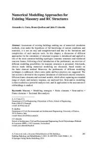
Water circulation and depth Figure 1 where u(x,y,t), v(x,y,t) are the velocity components, as shown in Fig.1 z(x,y,t) water elevation, h(x,y) the water depth, g gravitational constant acceleration, γ bottom friction coefficient,
f = 2ωsinφ coefficient of Coriolis force and H(x,y,t)=h(x,y)+z(x,y,t). 5. COLOURED VISUALISATION In this section we present a coloured analysis of the tide phenomenon of the S. Pablo Bay, visualising the data of sea elevation and velocity obtained by numerical simulation. In addition to show the behaviour of the phenomenon, this type of visualisation can be a precious and immediate tool to verify the solution of the adopted numerical model. To improve visual phenomenon knowledge we have realised colour scales, based on the HSL model and uniform colour model CIELUV. In scalar data representation, the simplest visualisation can be obtained displaying a single variable or parameter over a single image, but complex visualisations can be obtained displaying two or more parameters over a single spatial domain. The colour scales for single variable visualisation are ordinal and mainly formed by increasing (or decreasing) values of one component of a colour model. We have visualised the sea elevation computed at determined times t i i={1,..., 12} using the colour scales formed by increasing values of Hue component of the HSL model. Complementary-uniform colour scales used to visualise two parameters on a same image are computed in CIELUV model and generated in way that a variable y1 is mapped to lightness gradual steps of a colour c1(L*1,u*1v*1); while the value of the other variable y2 is mapped to lightness steps of the complementary colour c2(L*2,u*2v*2). As above mentioned, since complementary colours are colours which mixed in equal quantities give achromatic colours from black to white, the application of this type of scale leads to distinguish three main regions. The regions coloured in grey or achromatic colour denote equivalent values for the two variables. Areas coloured in dark grey correspond to low values of the variables, while zones of bright grey to high values. In the regions coloured by colours close to c1 the variable y1 is larger, while the zones where y2 prevails, are coloured by colours close to c2 [Levko97]. Analogous procedure has been realised to visualise three variables on the same image, but with the difference that the colour uniform scales computed in the CIELUV space and combined regard the primary colours R,G,B. Additive mixtures of equal quantities of primary colours R,G,B give achromatic colours from black to white. Also the vector data visualisation is a multiparametric visualisation since it involves representing data with multiple values at each sample point [Hesse94]. For the visualisation of two-dimensional vector data, techniques as arrows or streamlines can generate confused pictures
[Hall93] since these techniques typically consist in the projection of any icon onto screen, covering several pixels. In the case of arrows the direction is determined by the vector sum of the components and the length of the arrow is scaled by the maximum magnitude. The velocity can be visualised also by means of streamlines, which are lines everywhere tangential to the velocity. The latter visualisation offers a more global view of the flow, but the visual ambiguity and clutter remain. In Fig 2 and 3 we show the visualisation at time t=t1 of the velocity by means of arrows and streamlines. To avoid the drawback above mentioned, we used the colour tool also to visualise velocity data obtained by numerical simulation, implementing the circular look-up table of the colour wheel, as ordinal colour scale. This visualisation technique produces an image where the direction and/or magnitude of each vector is represented by colour [Johan95a] [Rhein95][Hall93].
Summing together the three colour components yields a colour that allows the values at three instants to be compared and analysed in qualitative and quantitative way. In Fig. 6 we have compared tide depths at t=t1 t=t 2 and t=t 3. Since the resulting colour in the combined image is mainly blue and cyan, that means tide elevations at times t=t2 and t=t3 are similar and both are higher than the elevation at time t=t1. The scales computed in CIELUV are generated in way that equal colour perceptual intervals ∆xi (distances) are assigned to the corresponding ∆yi distance of the numerical values. In the CIELUV scale computation there are projective transformations from every color ci (L*i, u*i,v*i) to tristimulus values X i,Yi,Zi and affine from Xi,Yi,Zi to R i,G i,B i that are the values to be addressed to the device. While in the perceptive scale generation of HSL space, the transformation of each colour from HSL co-ordinates to RGB coordinates is generally present in the hardware devices.
5. 1 SCALAR DATA VISUALISATION
5.2 VECTOR DATA VISUALISATION
As shown in Fig. 4, we show the behaviour of sea elevation at times t={t 1, ÉÉ, t12}. The scale is generated in HSL colour model varying the Hue component from blue to green and orange in order to describe the changes from low tide to high tide in the time. From t1 to t5 the tide elevation increases, from t6 to t10 the tide decreases and at time t11 and t12 starts to increase again. In Fig. 5 the changes of tide depth at times t= t1 and t =t4 are visualised on the same image. In this case we have generated uniform-complementary colour scale in CIELUV model using 3D Euclidean metric. The choice of uniform colour scale at perceptually uniform steps has been made for augmenting the quantitative information. The legend shows a final scale obtained combining the two uniform scales of the complementary colours of green and purple where the diagonal indicates a uniform grey scale from black and white corresponding equal contributes of complementary colours, while the sides denote the prevalence of the purple or green and their mixtures. The contribution of the colours of the two variables at each point are summed together to create the final representation. The final image is coloured by a colour scale that maps the variable at t=t 1 to purple colour component and the other at t=t 4 to green colour component. In the resulting image the prevalence of the purple colour shows the tide at time t=t1 is higher than that at time t=t 4 in the east side of the bay. The mapping of three scalar variables is realised colouring each scalar value with separated uniform scales of R,G,B, starting from black, computed in CIELUV.
The representation of velocity data requires to visualise together the variables of the direction and magnitude. We have utilised as ordinal colour scale, LHS colour wheel, that is a table of circular type with radial changes of colour. As shown in Fig 7, for each vector the colour wheel represents the direction by hue changing between [0o,360°] and the module by saturation changing between [0,100]. For example a pixel coloured by orange colour indicates the vector direction is from south-west to north-east in that point. The colour pictures of Fig. 8 a), b), c), d), e) and f) are obtained computing the solutions at time t=t 1, t=t 2, t=t 3, t=t 10, t=t11 and t=t12 respectively and show the periodic nature of the tide with T=12h. r The white colour represents velocity value v =0. In Fig 8 a), as it is indicated by the corresponding legend, the blue and cyan colours represent the magnitude and direction of sea velocities coming into the bay from east side; the orange and yellow colours describe the sea tide coming into the bay from south-west side; finally the green colour indicates the tide propagating towards north. Fig. 8 b), at t2 time shows the tide comes into the bay from only east side, and propagates towards south south-east. Fig 8 c), at t3 time, indicates, the sea tide comes into the bay from only east side and comes out to south-west side. In Fig 8 d) at time t=t10 the situation changes: the sea begins to come back from south-east side again. In Fig. 8 e), at t11 time, the tide comes into bay from south again. In Fig. 8 f) at time t=t12, we see the similar colours of the time t=t1 confirm the periodical nature of the phenomenon. The sea tide comes into the bay from east and south-west sides and diffuses towards north side.
The colour wheel of Fig. 9 uses an ordinal scale that emphasises the velocity directions from east side. We have only visualised the velocity directions which from the east side of the bay propagate to west, north-west and north sides at t=t1. The colour wheel of Fig. 10 uses a uniform scale, computed in CIELUV colour space at constant lightness. At t=t6 the image is depicted by hues representing the tide directions at constant lightness defining the velocity magnitude (lightness) included in the range [v1, v2]. The blue colour indicates the direction of the tide that starts from east side and has the magnitude in the predefined interval. The grey colour indicates velocity magnitude values are not included in the interval. In Fig. 11 we show two colour wheels using uniform and ordinal scales computed at two different levels of lightness. The dark scale represents the directions for values of the magnitude in the range [v1, v2] and light scale values in the range [v2, v3]. The grey colour indicates magnitude values not included in the intervals. The time instant is t=t4.
before. Our purpose is to obtain visualisation in steering phase, in which the modification of simulation parameters can be performed during the visualisation process. The software has been written in Mathematica 3. 0, but mainly C language in X windows environment under OS IRIX 6.2 on graphic workstation Silicon Graphics Octane /Si R10000 175 Mhz/ 128 Mb RAM. 7. REFERENCES [Coss97]
[Ebert00]
[Fairc97] [Gršll00]
6. CONCLUSION The results obtained by a finite difference method applied to the solution of 2D shallow water equations for the simulation of the real complex water circulation in the San Pablo Bay have been displayed by colour models. We have shown the colour can be a unifying tool to visualise both scalar and vector data generated from numerical simulation. In the representation of a single variable we have preferred to underline a qualitative reading of the sea elevation changes using perceptive colour space HSL. In the representation of two or more scalar variables on the same image, the use of uniform scales has emphasised equal values of the examined parameters, since perceptual distance between two colours corresponds to the Euclidean distance between their positions in the CIELUV space. In the velocity data representation we saw arrows or streamlines can render a confused image. For this reason we have utilised the colour wheel of the HSL model, that is a circular table taking into account the direction and magnitude have circular and radial nature respectively. Certain phenomenon features, such as periodic nature of the tide, can be easily identified with colour wheel. The use of the colour wheel permits to analyse the behaviour between flow directions in a time dependent simulation, as water circulation in the San Pablo natural basin. Visualisation has been performed in post-processing phase, when there is no direct interchange between the viewing and the simulation; the data have resulted from computer calculations done time
[Gross95] [Hall93] [Hesse94]
[Johan95a]
[Levko97]
[Macdo99]
[McCor87]
[Rhein95]
Cossu R. ÒVisual Exploration for Numerical Simulation DataÓ, Proceedings ESMÕ97, 11th European Simulation Multiconference, Istanbul, 84 Ð88, 1997. Ebert D. S.,Rohrer R. M., Shaw D. C., Pand P., Kukla J M., Roberts A. D., ÒProcedural Shape generation for multidimensional data visualisation , Data VisualisationÓ, Computer.& Graphics Vol. 24, pp 375-384, 2000. Fairchild M. D. ÒColor Appearance ModelsÓ, Addison Wesley Massachusetts Harlow 1997. Gršller E., Hauser Helwing, Ribarsky W., ÒData VisualisationÓ, Computer.& Graphics Vol. 24, pp 321-324, 2000. Gross M, Visual Computing, Computer.& Graphics Vol. 19, pp .34, 1995. Hall P. ÒVolume Rendering for Vector fieldsÓ, The Visual Computer 10 n. 3, 1993. Hesselink L., Post F. H.; van Wijk J.J.: ÒResearch Issues in Vector and Tensor Field Visualisation.Ó, IEEE Computer Graphics and Applications Vol. 14, n.2, pp 76-79.,1994. Johannsen A.and Moorhead R., ÒAGP: Ocean Model Flow Visualisation Ò , IEEE Computer Graphics and Applications Vol. 15 n. 7, July, 28-33, 1995. Levkowitz H., Color Theory and Modelling for Computer Graphics, Visualisation, and Multimedia Applications, Kluver Academic Publisher, Boston ,1997. MacDonald L. W ÒUsing Color Effectively in Computer GraphicsÓ, IEEE Computer Graphics and Applications Vol. 19, n.4, 2035,1999. McCormick B.H., De Fanti T.A., and Brown M.D., "Visualization in ScientificComputing," special issue, Computer Graphics, Vol. 21, No.6, Nov.1987. Rheingans P. and Landreth C.:Perceptual Principles for Effective
Visualizations. In Perceptual Issues in Visualisation, Georges Grinstein and Haim Levkowitz, eds. SpringerVerlag, 59-74, 1995 [Spita97a] Spitaleri R. M. Cossu R., Ò A Comparative Analysis of Reference Models for Visual and Computational Integrated EnvironmentsÓ, Computer & Graphics Vol 21 N. 5 1997 [Spita97b] Spitaleri R.M and Corinaldesi L., Ò A Multigrid Semi-Implicit Finite Difference Method for the TwoDimensional Shallow Water EquationsÓ, International Journal for Numerical Methods in Fluids V. 25, 112,1997 . [Telea99] Telea A., vanWijk J. J., ÒSimplified Representation of Vector FieldsÓ, Proceedings IEEE Visualisation 99. [Wisze82] Wiszecki G., and Stiles W.S.: Color Science: Concepts and Methods, Quantitative Data and Formulae, John Wiley & Sons, New York. 1982.
Sea elevation at times t1,É,t12 Figure 4
Sea elevation at times t1 and t4 Figure 5 Sea velocity at time t=t1 by arrows Figure 2
Sea velocity at time t=t1 by streamlines Figure 3
Sea elevation at times t 1 t2 t3 Figure 6
Colour wheel Figure 7 Selected direction of tide at t=t1 Figure 9
Sea direction at selected magnitude of velocity at t=t6 Figure 10
Sea velocity at time instants t1 t2 t3 t10 t11 t12 Figure 8 a) b) c) d) e) f) Sea directions at selected magnitudes of velocity at t=t4
Figure 11