combination of heterogeneous eeg feature ... - Semantic Scholar

Electronic version of an article published as [International Journal of Neural Systems, Volume 23, Issue 3, Year 2013, Pages 1350012 -20 pages] [DOI: 10.1142/S0129065713500123] © [copyright World Scientific Publishing Company] [http://www.worldscientific.com/worldscinet/ijns]

COMBINATION OF HETEROGENEOUS EEG FEATURE EXTRACTION METHODS AND STACKED SEQUENTIAL LEARNING FOR SLEEP STAGE CLASSIFICATION L.J. HERRERA1*, C.M. FERNANDES2,1, A.M. MORA1, D. MIGOTINA2, R. LARGO2, A. GUILLEN1, A.C. ROSA2 1

Computer Architecture and Technology Department, University of Granada, Spain * E-mail: [email protected] - Web: http://www.ugr.es/~jherrera 2 Laseeb, ISR-IST Technical University of Lisbon, Portugal This work proposes a methodology for sleep stage classification based on two main approaches: the combination of features extracted from electroencephalogram (EEG) signal by different extraction methods, and the use of stacked sequential learning to incorporate predicted information from nearby sleep stages in the final classifier. The feature extraction methods used in this work include three representative ways of extracting information from EEG signals: Hjorth features, wavelet transformation and symbolic representation. Feature selection was then used to evaluate the relevance of individual features from this set of methods. Stacked sequential learning uses a second-layer classifier to improve the classification by using previous and posterior first-layer predicted stages as additional features providing information to the model. Results show that both approaches enhance the sleep stage classification accuracy rate, thus leading to a closer approximation to the experts’ opinion. Keywords: Sleep Stage Classification, EEG, Feature Extraction, Feature Selection, Support Vector Machines.

automatic sleep classification is a hard computational problem that requires efficient solutions at different levels of the process, from feature extraction, passing through data analysis, to classifier design. Even though several attempts have been made in recent decades for automating the process, to our knowledge no method has been published that has proven its validity in a study including a sufficiently large number of controls and patients of all adult age ranges. The classification of sleep stages is frequently made under the Rechtschaffen and Kales36 (R&K) guidelines, which divide sleep into six stages: REM, NREM1, NREM2, NREM3 NREM4, and Awake (with REM meaning rapid eye movement, and NREM non-rapid eye movement). A recent classification proposal joins NREM3 and NREM4 in a single stage, reducing the number of stages to five21; other researchers, due to difficulties in differentiating light sleep stages (NREM1 and NREM2) and deep sleep stages (NREM3 and NREM4), use only four stages: light sleep, deep sleep, REM and Awake4,16. Most of the investigations that aim at automating sleep staging rely on polysomnography (PSG) 1,2,10, 14,15,17,22,29,39 , a multi-parametric test that monitors many

1. Introduction Sleep is a state of reduced and filtered sensory and motor activity, within which there are different stages, each one with a distinct set of associated physiological and neurological features. The correct identification of these stages is very important for the diagnosis and treatment of sleep disorders. However, sleep classification is not completely standardized and experts from different research centers may apply different criteria when deciding in which stage the patient is during a specific period of sleep. Even between expert co-workers there is usually less than 90% agreement in sleep classification32. Usually, sleep experts make the classification by means of visual methods, i.e., they analyze a set of signals that measure the patient’s body functions during sleep, and then, according to the signals’ patterns in a specific period, they decide in which stage the patient was in that precise period. This method is timeconsuming and prone to errors. Therefore, in biomedical sleep research it is very important to devise methods for extracting relevant information that may be later used for automatic classification of sleep stages. However, 1

2

L.J.Herrera, C. Fernandes, A.Mora et al.

body functions using electroencephalography (EEG), electromyography (EMG) and electrooculography (EOG) — although alternative procedures may be used4, they are not as reliable as PSG (or even EEG only). After extracting the relevant information from PSG signals, competent classification tools are required for a correct identification of the sleep stages. When available, EEG, EOG and EMG signals may be used, after a proper extraction of their features, as input for the classifier. However, PSG of the sleep is not always possible. Resource constraints restrict the access to complete sleep monitoring and there is a growing requirement for portable monitors that capture only the EEG signals from the patient and automatically classify the sleep stages. The EEG signal is similarly the most frequent source of information used in epilepsy studies3,5,13,49,50,53, Alzheimer’s disease54,58, and other brain-related diseases52. Automated sleep staging based on EEG signal analysis provides an important quantitative tool to assist neurologists and sleep specialists in the diagnosis and monitoring of sleep disorders, and the evaluation of treatment efficiency. In the literature, there is a wide range of different automatic methods developed for the purpose of supplying visual classification. These studies are normally focused either on the classification techniques or on novel feature extraction methods from PSG data. The evaluation of these systems typically use sleep data from a group of subjects, and then, either a random training-test subdivision of the selected dataset or a cross-validation approach, to quantify the classification accuracy rate. A different approach considers full patient hypnogram evaluation, by selecting training and test groups of patients or a patient-cross-validation approach. However, in general, we claim that the published results are hard to compare due to the heterogeneity of the data used and the variety in the experimentation design. This work first inspects the separate and joint use of heterogeneous feature extraction methods from EEG signals, using only this source of information for describing sleep. The three EEG feature extraction methods considered here are: the well-known Hjorth parameters19, an established method in sleep research; a wavelet transform feature extraction method proposed by Largo et al.27; and, finally, a recent method for new symbolic representation of sleep EEG proposed by Migotina31 that applies an optimal segmentation method

to each frequency band signal and segments the EEG signal29 for further symbolization. This work also presents the first complete and comparative results of this last method for sleep stage classification18. Before treatment, the available data is analyzed to check inter-class separability using Self Organizing Maps26. The relevance of each feature is then analyzed and a ranking is obtained through a well-known feature selection method called Normalized Mutual Information Feature Selection (NMIFS)12, which is based on the mutual information measure from Information Theory8. Support Vector Machines (SVM)37, a widely used highperformance classification paradigm, is the classification tool used in the experiments. SVM is also the basis to select features according to increasing performance in the classification. Finally this paper proposes a stacked sequential learning approach (SSL)7,47 to improve the classification results. This technique consists of a double-layer automatic classification framework, using the available set of features in an SVM classifier in the first layer, and using the predictions of this first classifier, for the epoch’s neighborhood, as additional features for a second-layer SVM classification process. Performance is in all cases evaluated using full patient hypnogram classification through patient-cross-validation. The convenience of the proposed approach is directly compared with classification systems based on a single EEG feature extraction method and with direct classification. Moreover, the SSL approach was compared with the known alternative for sleep stage classification using SVM classification to include context information, the SVM with posterior probability estimates approach16. Results show the superiority of the proposed methodology under the experimental setup presented. 2. Materials and Methods 2.1. Data In the proposed study, ten whole night PSG recordings (approx. 8 hours each) from healthy subjects of both genders (9 female, 1 male), aged 18-31 years old (mean: 23.7 ± 3.8), are used. The data was provided by Meditron Sleep Laboratory of the Neurology Department, State University of Sao Paulo, Botucatu, SP, Brazil18. Table 1 shows the number of distinct


epochs available from each subject’s recording. Each

3

sequential learning (section 2.6), performs a supervised

Fig. 1. Outline of the proposed sleep stage classification methodology.

epoch covers a non-overlapping period of 30 seconds. Table 1. Number of sleep epochs available for each of the 10 subjects. Subject #1 #2 #3 #4 #5 #6 #7 #8 #9 #10 Nº 812 901 762 842 749 788 839 666 813 859 epochs

All PSG recordings included EEG, EMG, EOG, ECG (electrocardiography) and respiration monitoring channels. EEG channels Fp1, Fp2, Fz, C3, C4, O1, O3 and Oz were recorded according to 10-20 international EEG system with reference to ears (M1 and M2). From each PSG recording, a single EEG channel (C3-M2) with a sampling frequency fs=128 Hz is used in the study. All EEG signals are cleared of high frequency noise (50-60Hz). Artifacts related to muscle/body movement and slow eye movement were removed by applying the automatic detection algorithm described in30, which is based on the application of a thresholding technique and histogram analysis of the EEG signal. Manual scoring of sleep stages according to Rechtschaffen & Kales criteria was performed by a very experienced sleep expert and provided for all subjects. 2.2. General Methodology Proposed Fig. 1 shows the proposed methodology outline for sleep stage classification from EEG signal data. First (section 2.3), EEG feature extraction methods are applied to extract the information from the signals, and these features are joined in a single feature vector per epoch. The supervised learning process makes use of the manually classified labels. Finally, stacked

classification learning process (based on SVMs in this paper, section 2.5) in two levels: a first one dedicated to initially estimate the sleep stage per epoch, and a second one that uses the same features plus the initially estimated stages in the nearby epochs to perform a final sleep stage classification for the current epoch. An intermediate feature analysis (section 2.4) identifies the most relevant features and the optimal subset of them to use in the classification (for both classifiers under the SSL approach). Unseen data classification would require the EEG extraction of the selected features by the feature selection algorithm, and the use of the double-layered SSL classification system to obtain the corresponding estimated hypnogram. Next sections present in detail each of the steps of the proposed sleep stage classification methodology. 2.3. Feature Extraction Methods 2.3.1. Segmentation of EEG signals Frequency Features Extraction At first, five most clinically relevant frequency bands 0 - 4 Hz (delta), 4 – 8 Hz (theta), 8 – 12 Hz (alpha), 12 – 16 Hz (sigma), and 16 – 20 Hz (beta) are extracted from each sleep EEG signal of a single channel C3-M2 by applying 8th order Butterworth FIR band-pass filter. The absolute value of each filtered EEG signal is then plotted, and in order to provide a smoother shape of the filtered signals, a linear interpolation method is applied between successive peak amplitude values on a wave-by-wave basis. This procedure has the effect of

4


smoothing the absolute valued signal in each band, so that it represents similar amplitude nearby waves as a single wave, whose shape is the linear interpolation of the their peak amplitudes. This step is essential for a later identification of these nearby similar amplitude waves as a single segment, according to the segmentation algorithm explained below. Details on this technique can be obtained from Migotina31. In the end, five frequency signals (delta, theta, alpha, sigma and beta) are obtained. Optimal Segmentation The optimal segmentation procedure29 is applied to each frequency signal obtained. The segmentation methodology is based on the calculation of optimal thresholds by maximum segments thresholding algorithm. Obtained threshold values are applied to the corresponding frequency signals for segmentation: all sample values exceeding the given threshold are considered as segments. This algorithm performs the analysis of segments density graphs29, and selects optimal thresholds in such way that it was possible to obtain maximum possible number of segments from each. The choice of the correct threshold is critical for the analysis, since it has direct impact in the output segmentation results. At the end, each frequency signal is described by the sequence of segments of the same type, i.e., delta frequency signal is represented by delta segments, theta frequency signal is represented by theta segments, and so forth. The proposed optimal segmentation algorithm is robust and allows overcoming the problem of signals’ normalization29. Combining Segments into Frequency Events The optimal segmentation algorithm provides five sequences of segments that correspond to different frequency signals. The next step is to combine segments from five sequences into a single sequence of frequency events. The combination procedure is based on an application of specified set of rules that takes into account information about duration of the segments and spaces between them. These rules were obtained heuristically and from the experts’ knowledge about sleep phasic events31. In total, thirty-one possible combinations of segments from the five bands (frequency events) are obtained for the whole EEG recording, and are finally quantified per 30-seconds epoch.

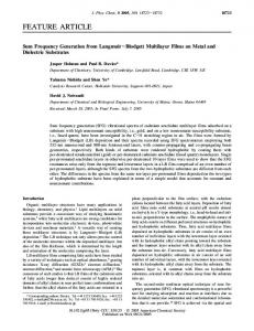
After the combination procedure a single sequence of frequency events that describes the sleep EEG signal is obtained. Each frequency event has two important parameters: the total number of events and their total duration (in seconds). In this work, only one parameter of frequency events, called duration, is used for the analyses. Please refer to Migotina31 for a detailed description of the segmentation and symbolic representation of the EEG. 2.3.2. Wavelets Wavelets are a class of functions used to localize a given function in both space and scaling. They are designed to have specific properties that make them useful for signal processing, and they have been applied to EEG processing in several fields of research, such as the identification of epileptic EEG signals49,51 and the diagnosis of Alzheimer’s disease54. In this work, using discrete Daubechies 6 (db6) wavelet, a multilevel wavelet packet transform28 was applied in order to obtain the single channel (C3-M2) EEG signal energy in the following five frequency bands27: beta=16-32Hz; sigma=12-16Hz; alpha=8-12Hz; theta=4-8Hz; delta=0.5-4Hz. Additionally the following four delta sub bands were calculated: slow-delta=0-0.5Hz; delta1=0.51Hz; delta2=1-2Hz; delta4=2-4Hz. In the next step, the mean powers of these bands in contiguous EEG 30s epochs were computed, using the coefficients from the wavelet packet transform. The resulting feature vector can be used to classify the sleep stage of each epoch and build the EEG sleep hypnogram (Fig. 2-a). The sleep EEG structure and the organization of frequency bands activity in each sleep state suggest the use of some other feature to increase stage discrimination36. We add to the feature vector some combinations of the original EEG bands: delta/(alpha+beta), alpha/(delta+theta), sigma/(alpha+beta), beta/delta and (slowdelta+alpha)/(delta+theta) (Fig. 2-b). Please refer to Largo et al. 27 for a detailed description of this feature extraction method. 2.3.3. Hjorth Parameters In 1970, Hjorth introduced a set of three parameters to describe the EEG signal in time domain19,41. These parameters are also called normalized slope descriptors because they can be defined by means of first and


second derivatives of the signal. As a reference method related to with higher order statistics of a signal, it represents a totally different nonlinear method from the two other methods proposed. The first parameter is a

(a)

5

where σa2 is the variance of the signal a, σd is the standard deviation (std.) of the first derivative of the signal, and σdd is the std. of its second derivative of. The dataset used in the experiment includes six additional features calculated from parameters activity and complexity. At first, Hjorth parameters are calculated through the whole EEG signal using a moving window with one second duration by applying discrete formulas (see Eqs. (1)-(3)). Two output signals corresponding to activity and complexity are then created. Mean, variance and std. of obtained signals are calculated for each 30 seconds epoch of analyzed sleep EEG signal. Thus, mean, variance and std. values of activity, complexity and mobility Hjorth parameters are used as features for sleep classification. 2.4. Feature Selection

(b) Fig. 2. Sleep hypnogram and wavelet parameters of one night sleep record. a) EEG bands power from the wavelet packed transform. b) Combined bands.

measure of the mean power representing the activity of the signal. The second parameter is an estimate of the mean frequency and is called mobility. The last parameter gives an estimate of the bandwidth of the signal. Since the computation of Hjorth parameters is based on variance, the computational cost of this method is considered low compared to other methods. Furthermore, the time domain orientation of Hjorth representation may be suitable for situations where ongoing EEG analysis is required. By definition, activity (m0), mobility (m2) and complexity (m4), are given by the following Eqs: 𝑚! = 𝜎! ! 𝑚! = 𝜎! 𝜎! 𝑚! = (𝜎!! 𝜎! )/ (𝜎! 𝜎! )

(1) (2) (3)

Feature selection is a key preprocess step in any classification problem11,34. It deals with the identification of the true relevancy of the factors (input features) with respect to the classification variable in a given problem. Its final objective is the selection of the smallest possible subset of features that provides the highest generalization capabilities to perform the classification. There is a wide literature on feature selection in machine learning research. One of the most widely used criterions to perform feature selection is the mutual information (MI) from Information Theory8, as it is able to identify nonlinear relationships between the features. Mutual information for two variables X and Y is calculated as: 𝐼 𝑋, 𝑌 =

𝑝 𝑥, 𝑦 log ! !

𝑝(𝑥, 𝑦) 𝑑𝑥𝑑𝑦 𝑝 𝑥 𝑝(𝑦)

(4)

In the case X or Y are discrete, the respective integrals are transformed into summations over the possible discrete values. The estimation of MI among features can be performed in several ways42: histograms, kernel density estimation, nearest neighbors, etc. This work uses the Fraser method12 that is based on the use of adaptive histograms for continuous features, and contingency tables for discrete features. The method has proven to behave robustly, independently of the type and values’ distribution of the variables involved12. From the Information Theory perspective, the objective of any feature selection algorithm is the reduction of the uncertainty (entropy) of the

6


classification variable with respect to the input features; or, similarly, the increase of the mutual information, by means of selecting the smallest and most relevant set of input features11. The requirement of relevancy directly relates to classifier higher performance; low dimensionality (avoiding unnecessary features) relates to higher generalization, faster model training and testing, and easier understandability of the model11. This tradeoff between relevancy and simplicity is a key issue in feature selection research. As stated above, there are several feature selection methods in the literature. Among them, we have chosen an enhanced method of the well-known minimumRedundancy Maximum-Relevancy (mRMR)35 algorithm, called Normalized Mutual Information Feature Selection (NMIFS)12, which uses the normalized MI measure by the maximum of the entropy of both sets of features: 𝐼(𝑋, 𝑌) (5) 𝑁𝐼 𝑋, 𝑌 = min {𝐻 𝑋 , 𝐻(𝑌)} The NMIFS method is an iterative methodology which returns a relevance ranking of the input features with respect to the classification variable, taking to account not only their importance, but also the redundancy among themselves. Thus, starting from an empty set of features S = {∅}, the NMIFS algorithm iteratively selects the input feature fi which maximizes: 𝐺 = 𝐼 𝐶, 𝑓! −

1 #𝑆

𝑁𝐼(𝑓! , 𝑓! )

(6)

!! ∈!

where #S is the cardinality of the current selected set S. The identification of the precise number of input features considered to perform the classification is normally performed by cross-validation evaluation of different classifiers (one per each possible number of input features considered). 2.5. SVM Classification Currently, SVM are probably the most frequently used classification paradigm in machine learning9,23,43,37. Binary SVM classification deals with the identification of the optimal largest margin classification hyper-plane in a dual space to separate the two classes involved. Multiclass classification in SVM is normally performed through the combination of a set of binary classifiers. The one-against-one approach constructs k(k-1)/2 classifiers, being k the number of classes, each one training a separating hyper-plane for two different

classes. Then, a voting scheme is used to identify the class to which each pattern belongs37. Among the kernel functions alternatives, Gaussian Radial Basis Function kernel has been chosen as it has proven to offer a good asymptotic behavior24. The estimation of the hyper-parameters of the SVM (C to control over-fitting, and γ to control the width of the Gaussian kernel) was done using grid search and crossvalidation37. Both hyper-parameters were logarithmically ranged between 2-15 and 25, in a 10x10 grid search. In the case of evaluating a large number of classifiers, however, this optimization technique can be computationally too costly. The Extreme Machine Learning approach points20 out that it is possible to obtain successful classification results by using reasonable values of hyper-parameters. Thus this last approach will be taken for the evaluations of the rankings returned by the feature selection algorithm, using as hyper-parameters values those returned by grid-search on a single execution on the complete dataset. The library LIBSVM6 for MATLAB® R2009a was used for the simulations. This library includes an implementation of the one-against-one approach for SVM multiclass classification, as well as efficient implementations of cross-validation and grid-search optimization techniques. 2.6. Stacked Sequential Learning One of the aims of this work is to evaluate the influence of nearby sleep stages information in the process of sleep stage classification. The hypothesis is that, in sleep stage classification, the present stage classification not only depends on the neuro-physiological signals of the current epoch, but also on the previous and posterior ones. That is, sleep experts not only take into account the EEG information (and other signals) of the current epoch to classify it, but also the previous (and following) behavior of the patient signals for identifying the precise stage. This context-based additional information can be considered in two ways: by including features from previous and posterior epochs in the classifiers, or, by including directly the previous and posterior estimated sleep stages to perform a subsequent, final classification. This second alternative is so-called Stacked Sequential Learning (SSL)7,47. It is a metalearning method in which the base classifier is


augmented by making it aware of the labels of nearby patterns for every input pattern. The proposed twolayered classification scheme can be seen in Fig. 3. As shown, the learning power of the classification system (in terms of classifier flexibility, information used for classification and potential accuracy) is ext

U

X

h1(X)

Y1

X

ext

h2(X )

Y2

Nb

Fig. 3. SSL scheme. The input features (X), and the labels (Y1) of a neighborhood (Nb) for each epoch, obtained in a first classification process h1(X), are considered as extended input data (Xext) for a second classification process h2(Xext), which obtains the definitive labels (Y2).

improved through the consideration of a neighborhood of initially estimated labels for every input pattern. In the problem we are dealing with, the neighboring labels are the previous and posterior firstly estimated stages (according to the patient’s first classifier h1(X) obtained hypnogram). Thus we are considering hypnogram context information that may be useful to improve the classification accuracy. This information should help avoiding isolated misclassified stages in the hypnogram; i.e. anomalous stage values with regard to its precedent and consequent stages. We have to recall that this behavior will be learned in a supervised manner and according to the experts’ knowledge, which previously scored the available data. Therefore, it is also to be noticed that it is not just a smoothing technique, as it would try to imitate the expert behavior. Then, if available data presents for instance isolated REM stages, they would be properly learned in the process and kept after SSL classification. This supervised learning process would help moreover, for instance using the performance estimation obtained by a crossvalidation process, to indicate the expectance that SSL improves the classification accuracy. In any case, it can be expected that an initial classification h1(x) providing accurate results will enhance the chances of success of the SSL approach.

7

3. Results This section describes the results attained in the set of experiments designed for this study. Four different tasks have been conducted. First, the available data is analyzed in order to assess the interclass distribution and separability. Then, the feature sets are joined and feature relevance is determined and evaluated. Classification performance is assessed, using SVMs, for the separate and joined feature sets, and for the relevance ranking of features. Finally, the classification results using context information through SSL are assessed. 3.1. Data analysis As mentioned above, patient-cross-validation (patientCV) is used here for performance evaluation of the different alternatives. In this approach, the available data from one patient Di is left aside as test data, while the information from the rest of patients is used to train the model; later the test data is evaluated using the learned model. This process is repeated for every available patient, and the expected performance of the evaluated methodology is the average performance over all the test executions. Standard deviations (std.) were also measured for each case. This patient-CV performance evaluation was strictly taken for all the simulations presented to assure an appropriate assessment of the different alternatives. Thus, for each fold, patient test data was always left aside in the application of the complete learning process of the different methods, and later tested. Comparison among different alternatives was assessed using a paired t-test (significance level α = 0.05) over the respective patientCV performances. Several preliminary complete simulations were done under other approaches to evaluate performance such as random training-test subdivisions of the complete dataset, random cross-validation under the complete dataset, and the use of a group of patients for training and other group for testing. However we detected a stronger data subdivision dependency under these performance evaluation frameworks, and it was decided to follow the patient-CV approach. We consider this performance measurement to be more robust and realistic in comparison with the other alternatives. Specifically, in comparison with random crossvalidation under the complete dataset, the alternative

8


taken considers the possible variable behavior in the hypnograms of different patients. Three subsets of features are available from three different feature extraction methods from EEG signals (see Section 2): EEG segmentation method, wavelets

pattern similarity (or, similarly, the overlapping among classes) was analyzed by means of Self-Organizing Maps (SOM). SOM26 is a feed-forward neural network that uses an unsupervised training algorithm and nonlinear regression techniques to learn or find

Fig.4. U-Matrix graph for all patterns and all features including the labels in the map cells (neurons). Intermediate cells plot the distances among the labeled ones, being close distances blue shades and far distances close to red tones. A detailed section with majority of cells labeled as classes NREM1-4 (numbered as 1-4 respectively, 5 is AWAKE and 6 REM) plotted separately. Looking at the figure it can be noticed that almost all the cells are blue, which means these cells are very close in the space, i.e. they (their codevectors) are quite similar. This reflects a great difficulty in correctly differentiating the patterns, and thus, in classifying them. Specifically and more clearly shown in the zoomed area, it is observed a strong proximity amongst classes NREM1 and NREM2 and class NREM3 with classes NREM2 and NREM4. This supports the convenience of joining classes NREM1 and NREM2 in LS and classes NREM3 and NREM4 in class DS in the study performed.

transformation method and Hjorth parameters. From them, respectively, the following continuous features are extracted (54 in total): 31 available features (named S1-S31) related to the duration of each frequency event group from the segmentation method; 14 features from the wavelet transform method (named W1-W14), corresponding to 5 bands and 4 sub-bands transforms, and 5 nonlinear transformations of the formers; 9 features corresponding to the mean, variance and std. of each of the three Hjorth parameters: activity (named H1-H3), complexity (named H4-H6) and mobility (named H7-H9). A preliminary analysis was performed in the data in order to evaluate the balance and overlapping among the different classes on the given dataset. The analysis shows that the number of samples in the classes is significantly unbalanced: classes NREM1, NREM3 and AWAKE showed to be less frequent than classes NREM2, NREM4 and REM. The expected inter-class

unknown relationships among the set of variables that describe a problem. The main property of the SOM is that it makes a nonlinear projection, based on pattern similarities, from a high-dimensional data space on a regular, low-dimensional (usually 2D) grid of neurons, called units. SOM uses a initialized 2D grid of neurons with random patterns within (called codevectors) and learns from the data by iteratively processing the input data and updating the nearest neuron codevectors (bestmatching units, BMU) in a similar-to clustering operation way (more details on the operation and parametrization of this technique can be found in26). This grid can be later processed to obtain the unified distance matrix (U-matrix)38 which helps detecting topological relations among neurons and inferring about the input data structure in a direct visual manner. U-matrix uses SOM yielded neurons’ codevectors (vectors of variables of the problem) as data source, and generates a matrix where each component is a distance


measure between two adjacent neurons. Then, these distances are codified as different color shades in a graph, and every neuron (cell in the graph) is labeled according the class of the majority of the input patterns whose BMU is the current neuron. Thus, high values (red-yellow shades in Fig. 4) in the U-matrix represent a frontier region between clusters, and low values (blue shades in Fig. 4) represent a high degree of similarities among neurons on that region, clusters. The SOM analysis was performed25 independently for each feature extraction method dataset and for the global set of features dataset. Fig. 4 plots the U-matrix graph for the global dataset, which clearly shows a strong overlapping between classes NREM1 and NREM2, as well as between classes NREM3 and both NREM2 and NREM4. This behavior was observed using any of the feature sets separately, so it was decided, in agreement with the sleep experts, and as done in previous works, to join classes NREM1 and NREM2 into class LIGHTSLEEP (LS)4,16 and classes NREM3 and NREM4 into class DEEPSLEEP (DS)21 to perform the classification. 3.2. Direct Classification Performance was evaluated both on the three groups of features separately, and in the joint set of features. This would assess the convenience of joining different and heterogeneous EEG-extracted feature sets to perform automatic sleep stage classification. Table 2 shows the patient-CV results obtained for the three separated feature sets, and for the joint feature set. Segmentation method features and wavelet transformation features showed similar performance, while the well-known Hjorth features showed a strong bias in patient-CV performance assessment. On the other hand, the joint feature set obtained the overall highest performance with a 75.86% of patient-CV accuracy. All performance differences were found to be significant by the paired ttest but the difference between the Segmentation Method and Wavelets Method. Table 3 shows the confusion matrix obtained for the patient-CV execution using the joint set of features dataset. It is observed a larger percentage overlap between classes AWAKE and LS, LS and DS and LS and REM. Class DS shows the highest classification performance while AWAKE stage shows the worst classification performance.

9

Feature selection was used to construct a relevance ranking of the variables on the joint dataset. These results are expected to provide information on the comparative importance of each of the three different feature sets. The feature selection NMIFS algorithm was tested in a double patient-CV scheme for the joint feature set data. This double cross-validation assessment system implies ten full 9-patient-CV runs of the feature selection method to select the optimal subset of features, leaving apart the left patient dataset as test. Due to this operation, the ranking obtained in each of the 10 runs may be different. Table 2. 10-patient-CV training and test accuracies for the three feature sets and joint feature set. Feature Extraction method Segmentation Wavelets Hjorth All features

10 patient-CV training accuracy (std.)

10 patient-CV test accuracy (std.)

74.82 (0.52) 76.36(0.51) 73.89(0.51) 80.85(0.60)

72.16(4.57) 72.27(7.59) 61.26(6.30) 75.86 (5.37)

Table 3. Confusion matrix for the joint set of features using patient-CV assessment. AWAKE

LIGHT DEEP REM TOTAL SLEEP(LS) SLEEP(DS)

%Acc

AWAKE

411

149

4

29

593

LIGHT SLEEP

69.30%

96

2867

348

432

3743 76.59%

DEEP SLEEP

18

427

1648

1

2094 78.70%

REM

30

381

6

1184 1601 73.95%

Fig.5. Mean results of a patient-CV execution of the NMIFS feature selection algorithm. For each optimal feature set size the mean cross-validation accuracy within the training dataset

10


of the ten executions is shown (blue line), as well as the crossvalidation test accuracy (red line).

Summarizing the results, Fig. 5 shows the average performance obtained in the variable selection approach for every possible optimal feature set; i.e., using the single best feature as feature set, the two most relevant features as feature set, the three most relevant features as feature set, and so forth, all according to the returned NMIFS ranking of features for each case. The figure shows the average training and test performance under the patient-CV approach, for each optimum combination of 1 to 54 possible features.

Table 4. Mean NMIFS feature ranking in the patient-CV execution: average highest to lowest relevant feature. Relevance rankings were averaged among the ten executions to obtain the average relative position. Std. is also provided for every feature. S1-S31 correspond to features from the segmentation method (with orange shading), W1-W14 to features from the Wavelets method (green shading) and H1H9 correspond to features from the Hjorth method (blue shading). It can be observed that features from the three methods appear in the highest relevancy ranking positions. Var S1 S2 H8 W11 S5 W13 S8 S26 S6 S4 S17 W9 S19 S7

𝑅𝑎𝑛𝑘(std) 2(1.1) 4.1(1.2) 4.3(2.1) 5.1(2.0) 6.5(5.7) 6.7(2.4) 7.3(2.8) 8.1(7.5) 8.8(1.5) 9.8(3.0) 9.8(3.2) 10.5(1.1) 11(2.3) 14.5(2.3)

Var H6 W14 W12 W7 H3 S3 H7 S16 W8 W6 W10 W1 W2 H1

𝑅𝑎𝑛𝑘(std) 14.7(6.9) 16.2(2.3) 16.4(1.1) 18.1(1.5) 19.5(1.3) 20.7(1.5) 20.7(1.4) 20.9(1.1) 23(0.7) 23.3(1.9) 25(0) 27(1.9) 27.3(1.3) 28(1.5)

Var H9 W4 H4 W3 H5 S13 S11 W5 S9 H2 S15 S10 S21 S31

𝑅𝑎𝑛𝑘(std) 28.8(0.6) 29.1(0.9) 30.8(0.4) 32(0) 32.7(6.6) 33.4(0.5) 35.2(2.1) 35.9(0.3) 36(1.4) 38(0) 38.8(0.6) 40(0) 41.2(0.4) 41.8(0.4)

Var S14 S23 S12 S29 S18 S28 S20 S27 S24 S22 S25 S30

𝑅𝑎𝑛𝑘(std) 43.7(0.9) 43.8(1.0) 44.9(0.7) 45.6(0.5) 47.2(0.2) 47.8(0.4) 49.5(0.5) 49.5(0.5) 51(0) 52.1(0.3) 52.9(0.3) 54(0)

the NMIFS algorithm under the patient-CV approach. For every variable, its average (and std.) ranking is shown. It can be seen from these results that the variable selection procedure is quite stable in the cross-validation execution (each possible group of nine patients), except for some features. The robustness is more noticeable as the relevancy of the variables diminishes (for instance, the least relevant, and the group of four least relevant features, coincide in all the executions). The mean optimum number of features selected by training CV evaluation is 37 (with std. of 5), being the mean training CV accuracy 81.27 and the

mean test CV accuracy 76.16, showing that there is a ratio of variables that introduce redundancy. 3.3. Stacked Sequential Learning Classification The use of SSL was evaluated according to the methodology presented in section 2.5, using a depth for SSL7 of 6. Optimal models obtained according to feature selection in section 3.2 were taken as first classifier h1(x) per each group of nine patients. Then, a second layer SVM classifier* receives as inputs the original features, plus a set of features indicating the initially estimated sleep stage for the current epoch and the 6 previous and posterior epochs (13 discrete + 54 continuous = 67 stages in total), using the optimal classifier obtained according to section 3.2. Second stage classifiers were again trained following the same patient-CV approach, using gridsearch and cross-validation for the obtaining of optimal hyper-parameters. It should be mentioned that, in principle, the starting and ending six epoch data of every hypnogram would be lost, as previous and posterior epoch sleep stage predictions are unavailable. However, as every original hypnogram starts and ends with AWAKE epochs, effective data size was kept, adding fake AWAKE estimated stages at the starting and end of every hypnogram. This SSL approach was applied to each of the feature extraction method dataset separately and on the joint feature dataset. Table 5 shows the patient-CV performances obtained with the proposed approach. An important increase in performance was observed for all cases, of about 4%-6%. Segmentation and Wavelets methods got higher performance results than Hjorth features, while the joint set of features got over 80% of accuracy. All performance differences among the alternatives in Table 5 were confirmed by the paired ttest, but again the difference between Segmentation method and Wavelets method in Table 5. Performance differences between the same methods with (Table 5) and without SSL (Table 4) were also statistically confirmed. Table 5. 10 patient-CV training and test accuracies, for the double-layered classification SSL approach for the three feature sets separately, and for the joint feature set.

*

For the SSL second layer classifier h2(xext), classes were encoded as {AWAKE = 1, LIGHT SLEEP = 2, DEEPSLEEP = 3, REM = 4}.


Feature Extraction 10-patient CV method training accuracy Segmentation method 78.13(0.47)

10 patient-CV test accuracy

Hjorth method All features

Table 6 shows the confusion matrix obtained for the patient-CV execution for the optimized classifier using the SSL approach for the joint set offeatures. It can be observed that the classification rate increases with this approach for all the sleep stages, in comparison with the direct classifier (see table 3). The LS stage got the highest classification accuracy (in contrast with the direct classification), and AWAKE remains getting the lowest classification accuracy. Table 6. Confusion matrix for the second stage SSL classifier. AWAKE

17.1(3.3)

H3

34(0.7)

S15 50.7(1.9)

76.41(5.18) 76.98 (7.93) 67.79(8.21) 80.07(6.02)

79.54(0.60) 74.95(0.82) 85.67(3.90)

Wavelets method

S26

11

LIGHT DEEP REM TOTAL %Acc SLEEP(LS) SLEEP(DS)

AWAKE

449

135

4

5

LIGHT SLEEP

593

75.71%

93

3075

297

278

3743 82.15%

DEEP SLEEP

18

427

1648

1

2094 79.13%

REM

29

299

1

1272 1601 79.45%

Table 7. Average highest to lowest relevant variables in the patient-CV execution for the second level SSL model. Ranking positions were averaged (including std.) to obtain a measure of relative relevancy. S1-S31 correspond to features from the segmentation method, W1-W14 to features from the Wavelets method, H1-H9 correspond to features from the Hjorth method and SS-6-SS+6 correspond to the first classifier outcome (SSL) features. In this case, SSL features are all selected first. Var 𝑅𝑎𝑛𝑘(std) Var 𝑅𝑎𝑛𝑘(std) Var 𝑅𝑎𝑛𝑘(std) Var 𝑅𝑎𝑛𝑘(std) SS0 1(0) S8 19.1(1.7) H7 34.8(0.6) H2 51.2(0.4) SS-3 2.1(0.3) S6 19.3(2) W8 36.1(0.6) S10 53.4(0.8) SS+1 3.6(0.8) S19 19.4(2.5) H9 36.4(7.9) S21 54.2(0.8) SS+6 4.1(1.2) W14 20.7(4.5) W6 36.8(0.4) S31 54.3(0.8) SS-1 4.2(0.4) S5 21.3(2.5) W10 38.2(0.4) S23 56.2(0.4) SS-2 6(0) S4 22.4(1.3) W2 39.4(1.4) S14 56.9(0.6) SS+2 7.1(0.3) S7 24.3(0.9) W1 40.6(1.8) S29 58.3(0.7) SS-4 7.9(0.3) W11 25.1(0.7) H1 41.4(1.7) S12 58.6(0.5) SS+3 9.2(0.4) W13 26.8(0.4) W4 42.5(0.8) S18 60.5(0.7) SS-5 9.8(0.4) W9 28.8(0.4) H4 44.5(0.8) S28 60.9(0.7) SS+4 11.2(0.4) S16 28.9(1.4) S13 45.7(2.2) S27 61.7(0.8) SS-6 11.8(0.4) S3 29.4(1.2) S9 46.6(2.6) S20 62.9(0.3) SS+5 13(0) H8 30.6(8.3) W3 46.6(0.5) S24 64(0) S2 15.4(1.3) H6 30.6(0.7) S11 48(2.8) S22 65.2(0.4) S1 15.7(0.9) W12 32(0.5) H5 48.5(0.5) S25 66(0.6) S17 16.2(2.3) W7 33(1.1) W5 49.8(0.8) S30 66.8(0.42)

Fig.6. Mean results of patient-CV execution of the NMIFS feature selection algorithm in the second-layer classifier in the SSL approach. For each optimal feature set size the mean cross-validation accuracy of the ten executions is shown (blue line), as well as the mean test accuracy (red line).

Variable selection was also applied to the second stage classifier, in order to assess the feature relevance of the SSL approach. In this case, there are four sets of features: segmentation method features, wavelet transformation features, Hjorth features, and previous and posterior epochs estimated stages features (those last labeled SS-6…SS0…SS+6, thus 67 in total). Fig. 6 shows the patient-CV training and test performances obtained, for each optimum combination of 1 to 67 possible features as mentioned. In this case, a larger variability on the results was observed with respect to the number of features chosen. The mean optimum number of features selected in this case by training CV evaluation was 46.5, with std. of 12.1, being the mean training CV accuracy 86.7% and the test CV accuracy 79.9% (similar to test CV accuracy using all features, also according to t-test). Table 7 shows the ranking average results, in which SSL features SS-/+𝜏 are selected as most relevant in all cases. Obviously feature indicating the sleep stage predicted by the first classifier h1(x) in the present epoch was chosen in all cases to be the most relevant one, obtaining a straightforward test accuracy of 76.16 (equal to performance of the optimal classifiers obtained as described in section 3.2). From the 14th feature, there is a higher variability in the ranking among the different cases, as well as in the difference between patient-CV training-test results.

12


4. Discussion There is an extensive literature on sleep stage classification techniques using PSG information. Most works propose new methods for extracting information from PSG signals, new algorithms for classifying the sleep stages, or frameworks that combine feature extraction methods and automatic classification tools. In general we can claim however that it is difficult to compare different approaches due to the different nature of the experiments performed, the existing difference among experts opinions32 which affect the information carried by data used in the supervised learning of the automatic classifiers, the use of different datasets for the comparisons, and the lack of specific and well-built benchmark datasets. In spite of this, an interesting brief survey on recent works for automatic sleep stage scoring can be found for instance in the work by Fraiwan et al.15. This work also presents a novel method using a continuous wavelet transform and linear discriminant analysis, using different mother wavelets to detect different waves embedded in the EEG signal, and improve the classification accuracy. The results attain an 84% on a cross-validation test over 32 subjects data. Figueroa Helland et al.14 also applied LDA in the problem of classification of sleep stages. They used additional information from ECG and respiratory channels in order to increase accuracy, and obtained results over a forward feature selection approach based on Wilk’s lambda as optimality criterion. The results are shown for a selected dataset on which a number of experts coincide in their manual scorings. Becq et al.45 compared the performance of five classifiers (linear and quadratic classifiers, k-nearest neighbors, Parzen kernels and Neural Networks) for automatic scoring of human sleep recordings. In order to evaluate the classifiers they used randomly drawn learning and testing sets of fixed size. Estimation of the misclassification percentage and its variability was obtained (optimistically and pessimistically). They also explored data transformations toward normal distribution as an approach to deal with extreme values. Classification accuracy ranged from 64% to 71% in the different classifiers on the transformed data, with the neural network getting the best classification accuracy on the validation set. Other recent works on new methods for feature extraction include the study by Rajendra et al.44. The

authors propose the use of higher order spectra to extract hidden information from the EEG signal. The authors show a promising classification accuracy using Gaussian mixture models of 88.7% over a dataset of 6198 sleep epochs. They also include a summary of results attained in previous works in the literature. An automated system for classification of human sleep stages based on hidden Markov models (HMM) was proposed by Doroshenkov et. al.10. The method obtains good results of automatic classification in agreement with the results of sleep stage identification performed by a sleep expert based on the R&K international system. HMM classification of stage 4 was 92% consistent with the R&K classification. The accuracy of classification of REM sleep was >86%. The worst accuracy of classification (