I would like to express my gratitude to my supervisors Ervin Gy®ri and Gá- bor Tardos for ..... After coloring it to a new color, delete it and do the same for the new ...
Combinatorial and computational problems about points in the plane By Balázs Keszegh
Submitted to Central European University Department of Mathematics and its Applications
In partial ful�lment of the requirements for the degree of Doctor of Philosophy (PhD) in Mathematics and its Applications
Supervisors: Ervin Gy®ri and Gábor Tardos
Budapest, Hungary January, 2009
Abstract We study three problems in combinatorial geometry. The problems investigated are con�ict-free colorings of point sets in the plane with few colors, polychromatic colorings of the vertices of rectangular partitions in the plane and in higher dimensions and polygonalizations of point sets with few re�ex points. These problems are problems of discrete point sets, the proofs are of combinatorial �avour with computational aspects and give e�cient algorithms. First we give a historical introduction to the topics and place our results in this context. We also investigate the similarities between the proving methods of the three topics. In the rest of the Thesis we present the results in all detail including proofs.
i
Acknowledgement I would like to express my gratitude to my supervisors Ervin Gy®ri and Gábor Tardos for shaping my areas of interest by discussing problems in extremal combinatorics and combinatorial geometry.
Their observations also improved
signi�cantly the presentation of this Thesis. I feel indepted for their and Gyula O.H. Katona's constant support to my research career, which was an essential help during my studies. I would also like to thank my co-authors for the many interesting discussions, �rst of all Eyal Ackerman, Dömötör Pálvölgyi and Géza Tóth, with whom I worked the most and further Oswin Aichholzer, Dániel Gerbner, Nathan Lemons, János Pach, Cory Palmer and Balázs Patkós. The mathematics Ph.D. program is a joint endeavor between the Rényi Institute of Mathematics and Central European University. I am grateful to both institutions. I would also like to thank the School of Computing Science at Simon Fraser University for having me as a guest in Vancouver during the Fall 2006 semester and also the Theoretical Computer Science Workgroup of Freie Universität and the Discrete Mathematics Workgroup of Technische Universität for having me as a guest in Berlin during the Fall 2007 semester.
ii
Contents 1 Introduction
1
1.1
Weak con�ict-free colorings
. . . . . . . . . . . . . . . . . . . . .
1.2
Re�exivity of point sets in the plane
1.3
Polychromatic colorings of rectangular partitions
. . . . . . . . . . . . . . . . . . . . . . . . .
2 Weak con�ict-free colorings 2.1
2.2
Bottomless rectangles
1 9 13
21
. . . . . . . . . . . . . . . . . . . . . . . .
21
2.1.1
Coloring points . . . . . . . . . . . . . . . . . . . . . . . .
21
2.1.2
Coloring bottomless rectangles
. . . . . . . . . . . . . . .
24
. . . . . . . . . . . . . . . . . . . . . . . . . . . . . .
31
2.2.1
Coloring points . . . . . . . . . . . . . . . . . . . . . . . .
31
2.2.2
Coloring half-planes
35
Half-planes
. . . . . . . . . . . . . . . . . . . . .
3 Re�exivity of point sets
40
3.1
Modi�ed Re�exivity and Iterative Subdivision . . . . . . . . . . .
40
3.2
A New Upper Bound . . . . . . . . . . . . . . . . . . . . . . . . .
43
3.3
Improving the Constant
. . . . . . . . . . . . . . . . . . . . . . .
44
3.4
An Algorithm . . . . . . . . . . . . . . . . . . . . . . . . . . . . .
46
3.5
Discussion and Open Problems
50
. . . . . . . . . . . . . . . . . . .
4 Polychromatic colorings of rectangular partitions 4.1
Polychromatic colorings of planar rectangular partitions
4.2
Polychromatic colorings of
n-dimensional
54 . . . . .
guillotine-partitions
. .
54 64
5 Concluding remarks
73
Appendix
75
Bibliography
80
iii
1 Introduction In this thesis we study several problems in
combinatorial geometry.
The
problems investigated are con�ict-free colorings of point sets in the plane with few colors, polychromatic colorings of the vertices of rectangular partitions in the plane and in higher dimensions and polygonalizations of point sets with few re�ex points. The connections between these problems might not be obvious at �rst sight as the historical relation between them is not very strong.
Instead,
many similarities between the proving methods can be observed. All problems are
problems of discrete point sets,
and are problems in
the proofs are of combinatorial �avour
computational geometry with algorithmic proofs.
First
we overview the topics and the results appearing in the Thesis. Finally, we give a more detailed overview of the methods appearing in the proofs.
1.1 Weak con�ict-free colorings The following problem is the meeting point of two areas of combinatorial geometry.
The �rst and older of these two is the problem of
decomposability of
multiple coverings (and the closely related problem of multiple packings which we do not discuss here), the other one is
con�ict-free coloring
of points and
regions. We start with the introduction of the �rst one. Multiple coverings (and packings) were introduced independently by Davenport and László Fejes Tóth. Given a system
k -fold F
of subsets of an underlying set
covering if every point of
P
k = k(F)
such that any
P,
belongs to at least
of regions in the plane is called
integer
F
F
we say that they form a
k
cover-decomposable
k -fold
members of
F.
A family
if there exists a positive
covering of the plane with members from
can be decomposed into two coverings (i.e. into two
1-fold
coverings). In an
unpublished manuscript, P. Mani-Levitska and Pach [35] showed that every
1
33-
fold covering of the plane with congruent open disks splits into two coverings, thus the set of the translates of an open disc is cover-decomposable. Pach [37] also showed that the set of the translates of any open centrally symmetric convex polygon is cover-decomposable. Tardos and Tóth [47] extended this result to any open triangle. Recently Pálvölgyi and Tóth [43] extended this result further to any open convex polygon. Pach et al. [40] proved several negative results, among others they proved that the set of translates of any concave quadrilateral is not cover-decomposable. One important observation is that to prove cover-decomposability, it is enough to solve a �nite problem, as for open bounded sets it implies the cover-decomposability. This
�nite-cover-decomposability
means that having an arbitrary �nite subset of
the given set of regions we need a two-coloring of these regions such that any
k -fold
covered point is covered by regions of both colors. For example the set of translates of an arbitrary open convex polygon is �nite-cover-decomposable as well [43]. Recently Pálvölgyi [42] showed that the set of translates of any general (having no parallel edges) concave polygon is not �nite-cover-decomposabe. He also characterizes which non-general concave polygons are �nite-cover-decomposable and which are not thus answering the �nite question for every open polygon. The other important observation used throughout these proofs is that it is possible to consider the following dual problem. Distinguish an arbitrary point in a center (if system
S.
S
S
S
as
is centrally symmetric let it be its real center) and then for a given
of translates of
Clearly,
S
forms a
S,
let
k -fold
C(S)
denote the set of centers of all members of
covering of the plane if and only if every translate
of
−S
S
to its center, thus for centrally symmetric
contains at least
k
elements of
C(S)
(where
S
−S
denotes the re�ection of
we have
−S = S ).
I.e.
cover-
decomposability is equivalent to the existence of a bipartition (two-coloring) of these points such that every translate of both parts (colors).
2
−S
contains at least one element from
The dual of the �nite-cover-decomposability problem is that having a �nite set of points we need a two-coloring of the points such that any translate of at least
k
−S
covering
of these points covers points of both colors. This �nite dual version can
be phrased for any set of regions, not just for the set of translates, in this case the two versions are not equivalent (for example for all discs of the plane it does not hold). Given a family of regions and a �nite subfamily of Smorodinsky [46] one can de�ne the base set is the set of regions there is a hyperedge
rp
F
F
of it, following the notation
geometric hypergraph
and for any point
p
induced by
covered by at least
containing the regions covering
p.
k
F.
The
regions
A proper coloring of
a hypergraph is a coloring of the points such that there are no monochromatic edges. Clearly, determining whether there is a proper two-coloring for any �nite subfamily
F
is equivalent to the �nite-cover-decomposability de�ned above. The
dual problem can be phrased similarly as a hypergraph-coloring problem. Then it is natural to ask what is the minimal number of colors for which a proper coloring exists. This is where we arrive to the notion of weak con�ict-free colorings but before de�ning it in whole generality we have to talk about the other area it relates to, the area of
con�ict-free colorings, which serves as the main
motivation to investigate these questions. Motivated by a frequency assignment problem in cellular telephone networks, Even, Lotker, Ron and Smorodinsky [23] studied the following problem. lular networks facilitate communication between �xed
clients.
base stations
Cel-
and moving
Fixed frequencies are assigned to base-stations to enable links to clients.
Each client continuously scans frequencies in search of a base-station within its range with good reception. The fundamental problem of frequency assignment in cellular networks is to assign frequencies to base-stations such that every client is served by some base-station, i.e. it can communicate with a station such that the frequency of that station is not assigned to any other station it could also
3
communicate with (to avoid interference). Given a �xed set of base-stations we want to minimize the number of assigned frequencies.
First we assume that the ranges are determined by the clients, i.e. if a basestation is in the range of some client, then they can communicate. Let
F
set of base-stations and some family
F
P
the family of all possible ranges of any client. Given
of planar regions and a �nite set of points
P
we de�ne
cf (F, P )
as the smallest number of colors which are enough to color the points of that in every region of
F
be the
P
such
containing at least one point, there is a point whose
color is unique among the points in that region. The maximum over all point sets of size
n
is the so called
denoted by
cf (F, n)
cf -colorings
con�ict-free coloring number (cf-coloring in short),
(for a summary of the de�nitions of the di�erent versions of
see De�nition 1.1). Determining the cf-coloring number for di�erent
types of regions
F
is the main aim in this topic. Regions for which the problems
has been studied include discs ([23], [46], etc.) and axis-parallel rectangles ([16], [41], [7], etc), we give a more detailed overview after introducing the de�nitions needed. It is natural to de�ne a dual version for con�ict-free colorings as well. It is natural to assume that the ranges are determined by the base-stations, i.e. if a client is in the range of some base-station, then they can communicate. For a of planar regions
F
we de�ne
cf (F)
enough for coloring the regions of
F
�nite
family
as the smallest number of colors which is such that for every point in
∪F
there is a
region whose color is unique among the colors of the regions covering it. For a (not necessarily �nite) family
F
of planar regions let
cf (F, n),
the
con�ict-free
region-coloring number of F be the maximum of cf (F 0 ) for F 0 ⊆ F , |F 0 | = n. Smorodinsky [45] and then Har-Peled et al. [27] de�ned generalized versions of these notions. A
F
of
F
cfk -coloring of a point set is a coloring such that for each region
containing at least one point, there is a color which is assigned to at most
4
k
points covered by
F.
Note that a
cf -coloring
is actually a
cf1 -coloring.
The
region-coloring version is de�ned similarly.
De�nition 1.1.
Given a family F of planar regions and a �nite set of points P ,
• cfk (F, P ) = min c: ∃ c-coloring f of P s.t. ∀F ∈ F ∃x s.t. 1 ≤ |{p : p ∈ F, f (p) = x}| ≤ k • cfk (F, n) = max|P |=n cfk (F, P ); cf (F, n) = cf1 (F, n) • if F is �nite, cfk (F) = min c: ∃ c-coloring f of F s.t. ∀p ∈ ∪F ∃x s.t. 1 ≤ |{F, p ∈ F, f (F ) = x}| ≤ k • cfk (F, n) = max|F 0 |=n,F 0 ⊂F cfk (F 0 ); cf (F, n) = cf1 (F, n) Now we arrived to the point where we can introduce the notion of
con�ict-free colorings. di�erent versions of
For a summary of the forthcoming de�nitions of the
wcf -colorings
of a con�ict-free coloring,
P,
it covers
The maximum over all
2 n
see De�nition 1.5.
wcf (F, P )
needed to color the points of points of
weak
P
Modifying the de�nition
equals to the minimum number of colors
such that whenever a region covers at least
of di�erent colors (the region is element point set of size
n
is the
2
not monochromatic).
weak con�ict-free
coloring number (wcf-coloring in short), denoted by wcf (F, n). Observation 1.2.
cf (F, n) ≥ wcf (F, n).
Generalizing our de�nition we can de�ne of colors needed to color the points of least
k
points of
P,
then it covers
2
P
wcfk (F, P ) as the minimum number
such that whenever a region covers at
points of di�erent colors.
of this value over all point sets of size
n
is denoted by
The maximum
wcfk (F, n).
Note that
wcf (F, n) = wcf2 (F, n).
Observation 1.3.
wcfk (F, n) ≤ wcfl (F, n) if k ≥ l.
Even et al. [23] presented a general algorithmic framework on con�ict-free colorings, re�ned version of this approach appeared in [27] (and later in [46]) where
5
they summarized it in a lemma showing essentially that the weak con�ict-free coloring number gives a good upper bound to the con�ict-free coloring number (they do not use the notation
wcf -coloring
and they deal only with the case
k = 2).
The algorithm giving a con�ict-free coloring from weak con�ict-free colorings is the following. In each step take a biggest color class in a weak con�ict-free coloring of the point set. After coloring it to a new color, delete it and do the same for the new (smaller) point set.
This framework also works for
wcfk -coloring
easy to see that taking in each step a color class of a
cfk−1 -coloring.
Lemma 1.4.
k > 2
as it is
we get a
The generalized version of the lemma stated in [27] is as follows.
For any �xed k ≥ 2
(i) if wcfk (F, n) ≤ c for some constant c, then cfk−1 (F, n) ≤
log n log(c/(c−1))
=
O(log n),
(ii) if wcfk (F, n) = O(n� ) for some � > 0, then cfk−1 (F, n) = O(n� ). Observation 1.2 and Lemma 1.4 show that each other. Often the best known bound for
cf
wcf
and
cf
are usually close to
is obtained from Lemma 1.4. This
is the main motivation why we want to determine the weak con�ict-free coloring number for di�erent types of regions. As this lemma gives bound for
wcfk ,
it motivates the investigation of
wcfk -colorings
Again we can de�ne the dual version. For a �nite
for
F , wcf (F) equals to the smallest
F
is the
F
F
such that
2 regions in F , there are two di�erently colored
regions among the regions covering it (the point is necessarily �nite
using
k > 2.
number of colors which are enough to assign colors to the regions in for every point covered by at least
cfk−1
not monochromatic).
the maximum of this value over all
n
For a not
element subfamilies of
weak con�ict-free region-coloring number, denoted by wcf (F, n).
Finally, we can again de�ne covered by at least
k
wcfk (F, n) by restricting the condition only for points
regions in
F.
The dual version of Lemma 1.4 holds as well.
Let us recall the geometric hypergraph de�ned earlier. Given a �nite family of
6
regions
F,
any point
p
covered by at least
regions covering
p.
k
regions there is a hyperedge
for which
rp
and for
containing the
We were interested in determining its chromatic number,
which is clearly equivalent to determining
k
F
the base set of the hypergraph is the family of regions
wcfk (F) = 2
wcfk (F).
Further, the existence of a
is equivalent to the statement that
F
decomposable. Indeed, a good weak con�ict-free region-coloring of
is �nite-cover-
F
gives a good
partition and vice versa. In the dual version such equivalence holds as well. For most regions we study, the weak con�ict-free coloring number can always be bounded from above by a constant not depending on de�ne
wcfk (F) = maxn wcfk (F, n)
if they exist.
and similarly
n.
Thus, for in�nite
F
we
wcfk (F) = maxn wcfk (F, n)
Our main aim is to determine these numbers and give coloring
algorithms using this minimal number of colors. Before doing so, let us collect here the de�nitions of the di�erent versions of
De�nition 1.5.
wcf -colorings.
Given a family F of planar regions and a �nite set of points P ,
• wcfk (F, P ) = min c: ∃ c-coloring f of P s.t. ∀F ∈ F if |{p : p ∈ F }| ≥ k
then ∃p, q ∈ P, p 6= q : p, q ∈ F and f (p) 6= f (q) • wcfk (F, n) = max|P |=n wcfk (F, P ); wcf (F, n) = wcf2 (F, n) • if F is in�nite, wcfk (F) = maxn wcfk (F, n), if it exists • if F is �nite, wcfk (F) = min c: ∃ c-coloring f of F s.t. ∀p ∈ ∪F if |{F : p ∈ F }| ≥ k then ∃F, G ∈ F, F 6= G : p ∈ F, G and f (F ) 6= f (G) • wcfk (F, n) = max|F 0 |=n,F 0 ⊂F wcfk (F 0 ); wcf (F, n) = wcf2 (F, n) • if F is in�nite, wcfk (F) = maxn wcfk (F, n), if it exists Slightly modifying the notation of [27] we call a family of regions if for any �nite
P, F ∈ F
then there exists
F0 ∈ F
and
l
positive integer if
covering exactly
7
l
F
points of
F
covers at least
P,
l
monotone points of
all covered by
F
F
as well.
Observation 1.6.
For monotone families of regions in the de�nition of wcf-
coloring it is enough to restrict our condition to regions covering exactly 2 points of the point set. Similarly, for the de�nition of wcfk it is enough to restrict the condition to regions covering exactly k points. Note that monotonicity could be de�ned in the dual version as well, but none of the types of regions we study are monotone in that dual sense. Let us now summarize the results known about axis-parallel rectangles and discs (the two most widely examined region types) and pose open problems regarding the unsolved cases. The general case of axis-parallel rectangles (denoted by still far from being solved, the best bounds are
R) is
n wcf (R, n) = Ω( (loglog ) by Chen log n)2
˜ .382+� ) wcf (R, n) = O(n q log n wcf (R, n) = O( n log log n ) by Pach
et al. [16] from below and recently by Ajwani et al. [7] from above, improving the previous bound
et al. [41]. So probably one of the most interesting problems is still to give better bounds for
n
wcf (R, n),
i.e. the lowest number of colors needed to color any set of
points, such that if an axis-parallel rectangle covers at least two of them then
not all of those covered by it have the same color. For the dual case of coloring axis-parallel rectangles the proof of the upper bound
cf (R, n) = O(log2 n) wcf (R, n) = O(log n).
([27]) can be modi�ed easily to give the upper bound There is a matching lower bound
by Pach et al. [39]. This implies the same lower bound for
wcf (R, n) = Ω(log n) cf (R, n),
thus in this
case there is still a slight gap between the lower and upper bounds. The case of discs (denoted by
D)
in the plane is only partially solved.
It is
easy to see that a proper coloring of the Delaunay-triangulation of a point set gives a weak con�ict-free coloring. From the four-color theorem we conclude that
wcf2 (D) = 4.
Further, Pach et al. [40] showed that
Problem 1.7.
wcfk (D) > 2
for any
k.
Is it true for some k that wcfk (D) = 3? If yes, �nd the smallest
such k . Answering the question if
wcfk (D) exists for some k
8
Smorodinsky [46] showed
k
2
3
≥4
wcfk (B)
3
3
2
wcfk (B)
3
2
2
wcfk (H)
4
2
2
wcfk (H)
3
2 or 3
2
Table 1: table of results about B and H that
wcf2 (D) = 4.
Problem 1.8.
Give better bounds for wcfk (D) when k > 2.
Now we can summarize the new results presented in Chapter 2. In Section 2.1 we solve all cases for rectangles. A
x < b, y < c by
B.
bottomless rectangles,
bottomless rectangle
for some
a, b
and
c.
a special case of axis-parallel
is the set of points
(x, y)
such that
a
2.
12
point construction on Figure 4(a) cannot be colored with
any bottomless rectangle covering at least
3
For that we show that the
2
colors such that
points covers two di�erently colored
points. Suppose on the contrary that there is such a coloring. Denote the points ordered by their points
p4 , p 5 , p 6
is red. If
p4
and
x-coordinate
from left to right by
p1 , p2 , . . . , p12 .
there are two with the same color, wlog. assume that this color
p5
are red, then all of
rectangle covering only
p4 , p 5
p1 , p 2 , p 3
are blue as there is a bottomless
and any one of these
3
points. This is a contradic-
tion as there is a bottomless rectangle covering only these
p4
and
p6
are red then similar argument for the points
are red then similar argument for the points
(ii)
Among the
p7 , p 8 , p 9
3
points, all blue. If
p10 , p11 , p12 ,
if
p5
and
p6
yields to a contradiction.
We want to color the points red and blue such that any bottomless rect-
angle covering at least
4
points covers two di�erently colored points.
First we color the lowest point of
P
red then we consider the points in upwards
22
p7
p3
p8 p2 p9
p1 p5
p10 p11 p12 p6
p4
(a) Theorem 2.1(i)
(b) Theorem 2.2(i)
Figure 4: Lower bound constructions for bottomless rectangles order.
We do not color every vertex as soon as it is considered.
that in the
x-coordinate
We maintain
order of the points considered so far there are no two
consecutive uncolored points and the colored points alternate in color. When a new point is considered we keep it uncolored unless it has an uncolored left or right neighbor (note that it cannot have both) in the
x-coordinate
order. In that
case we color the new point and its uncolored neighbor in a way that keeps the alternation. At the end we arbitrarily color the remaining points in
P.
Now we
only need to prove that this coloring is good. Consider a bottomless rectangle covering at least considered
B ∩P
4
points. Let
p
be the highest point covered by
B.
When
p
B is
is an interval in the left to right order of the points considered so
far. By the properties maintained any such interval of at least
4 vertices contains
both red and blue points as needed.
(iii) We need to prove that the algorithms presented in the proof of Claim 2.1 and Theorem 2.1 points takes
(ii) run in time O(n log n).
O(n log n)
each computable in
Computing the upwards order of the
time, the rest of the algorithm has
O(log n) time,
n
steps in both cases,
in the latter algorithm there is a �nal coloring
step that takes at most linear time, so the whole algorithm runs in time in both case.
23
O(n log n)
2.1.2
Coloring bottomless rectangles
In [46] a very similar version is considered, namely, weak con�ict-free coloring of axis-parallel rectangles intersecting a common base-line. The proof of their result with a slight modi�cation gives
wcf k (B)
for every
k,
wcf2 (B) ≤ 4.
The following theorem determines
also improving this bound to
3
colors, which is optimal.
From now on we assume that there are no two bottomless rectangles with overlapping sides. It is easy to show that if this is not the case, then coloring the rectangles after perturbing them such that afterwards there are no overlappings, gives a needed coloring for the original family of rectangles as well.
Theorem 2.2. (i) wcf2 (B) = 3 i.e. any family of bottomless rectangles can be colored with 3 colors such that any point covered by at least 2 of them is not monochromatic. (ii) wcf3 (B) = 2 i.e. any family of bottomless rectangles can be colored with 2 colors such that any point covered by at least 3 of them is not monochromatic. (iii) Such colorings can be found in O(n2 ) time. Proof. (i)
For the lower bound, the arrangement of
shows that
3
3
rectangles on Figure 4(b)
colors are sometimes needed. For the upper bound, given a fam-
ily of rectangles with a common base line we want to color the rectangles red, blue and green such that any point covered by at least
2
rectangles is covered by
two di�erently colored rectangles. We color the rectangles in downwards order according to their top edge's
y -coordinate.
We start with the empty family and
reinsert the rectangles in this order. We color the �rst, i.e. the highest rectangle blue. After each step we have a proper coloring and we preserve the following additional assumption. If a point on the base-line is covered by exactly
1
rectan-
gle, then it is not red. In each step we insert the next rectangle
B
in downwards order, so its top edge
is below the top edge of all the rectangles already inserted. We color
24
B
red. We
2. red-green 1. blue-green
B s
q
base-line
blue interval
Figure 5: The color switches of the `divide and color' method in Theorem 2.2(i). claim that this is again a proper coloring. Indeed, the condition for points not in
B
already holds. For any point covered by
B
the base-line point with the same
x-coordinate is covered by the same rectangles as B
is the lowest rectangle. Thus,
it is enough to check the condition for base-line points in by at least
2
covered by
B,
rectangles besides
B
B.
If a point is covered
then it is good by induction. Otherwise it is
which is red and exactly one more rectangle, which is not red by
the assumption. If there is no base-line point covered by only holds too.
If
q
B,
then the additional assumption
is such a point then we need to do something else to maintain
the validity of our assumption. If a base-line point is covered by only
1
rectangle
then we say that the color of this point is the color of the rectangle covering it. It is easy to see that if there is such a point
p and we switch the other two colors on
the rectangles completely to the left (or to the right) to
p,
the coloring remains
good. With only such `divide and color' steps we will change the coloring such that there will be no point on the base-line covered by exactly
1
green rectangle.
Finally we will switch the colors green and red on all the rectangles to have a good coloring satisfying the assumption.
For an illustration of the rest of the
proof see Figure 5. In the current coloring all green base-line points are left or right to
25
B
as
B
is red.
B2
B2
B2
B1
B1
B1
q
Figure 6: The division of the `divide and color' method in Theorem 2.2(ii). We will deal with the left side �rst, changing the colors only of rectangles strictly left from
q
and making a good coloring satisfying the condition for any base-line
point left to
q.
On the right side we proceed analogously, changing the colors
only of rectangles strictly right from
q
and making a good coloring satisfying the
condition for any base-line point right to
q.
This way we get a good coloring
satisfying the assumption for all base-line points. On the base-line to the left of
B
there are some intervals of single colored points,
all of them green or blue. If there is no green one then we are done. Otherwise, we can suppose that the closest such interval to
B
blue and green on the rectangles strictly left from
is blue, otherwise switch colors
q,
still having a good coloring.
Now switch colors red and green on the rectangles strictly left from any point
s of
this blue interval, this way we got rid of all green points, making the assumption true for all points left to
(ii)
B.
This concludes the proof.
Given a family of rectangles with a common base line we want to color
them red and blue such that any point covered by at least
3 rectangles is covered
by two di�erently colored rectangles. Moreover, the coloring we got will always satisfy the following additional assumption. Any point on the base-line covered
by exactly
2
rectangles is covered by a red and a blue rectangle.
Now we need a di�erent version of the `divide and color' method. We will proceed by induction on the number of rectangles. A single rectangle is colored red. In a general step �rst assume that there is a point
q
on the base-line not covered by
any rectangle and there are some rectangles strictly left and strictly right from
26
that point too. Color the rectangles to the left of
q
and the ones to the right of
separately by induction, putting these together this is clearly a good coloring.
Now assume that there is a point
B
q
q on the base-line covered by exactly 1 rectangle
and there are some rectangles strictly left and strictly right from that point
q
too. Color �rst the rectangles to the left of
B.
to the right together with
B
together with
then the rectangles
As there were some rectangles on both sides, this
can be done by induction. By a possible switching of the colors in the left and right parts,
B
is red in both colorings. Putting together the two half-colorings
we get a good coloring. The next case is when we have a point two rectangles,
B1
and
B2
q
on the base-line covered by exactly
(see Figure 6 for an illustration)and there is at least
q.
one rectangle both to the right and to the left of induction the rectangles strictly left from Using the assumption on
q
we see that
q
B1
In this case color �rst by
together with these two rectangles.
and
B2
have di�erent colors, after a
possible switch of the two colors we can assume that
B1
is red and
The same way we color the rectangles strictly right from
q
B2
is blue.
together with these
two rectangles. This way the two rectangles are colored with the same colors in both colorings and so we can put together these two half-colorings (if none of them is empty) to have a coloring of the whole family of rectangles. This coloring is good by induction. In the remaining case for any base-line point covered by exactly
1 or 2 rectangles,
there is no rectangle strictly to the left or to the right to that point. The left and right sides of the rectangles divide the base-line into
2
half-lines and
2n − 1
intervals. It is easy to see that in this case the only base-line points covered by exactly
1
rectangle are the points of the leftmost
L1
and rightmost
and the 2-covered points are the points of the second leftmost rightmost
R2
L2
R1
interval
and second
interval. Consider rectangle
B,
the one with the lowest top edge.
1-
or
2-covered
It is easy to see that if it does not cover
27
base-line points then we
can color the rest of the rectangles by induction and then color
B
with arbitrary
color not ruining the coloring and the additional assumption. Otherwise
covers
L1 , L2 , R1 , R2 .
some intervals from If it covers some of
L1
and
L2
other rectangle covering
L2 ,
R1
and does not cover
B
rest of the rectangles by induction and then color
and
R2
then color the
to a di�erent color from the
this way we obtain a good coloring satisfying our
additional assumption. If it covers some of
L2
B
R1
and
R2
and does not cover
L1
and
then a symmetrical argument gives a good coloring.
It remains to deal with the case when the rectangle
covers
L2
and
R2
as well. Consider now
with the second lowest top edge. First assume that
L1 , L2 , R1 , R2 .
cover any of
B)
B2
B
B2
does not
In this case color the rest of the rectangles (including
B2
by induction and then color
with the same color as
B.
coloring is good. Any point ruining the condition must be in contrary that there is a point
p
covered by at least
3
We claim that this
B2 .
Assume on the
rectangles all having the
same color. If
p
is covered by
3
rectangles besides
B2
then by induction there are di�erently
colored rectangles among these, a contradiction. If
p
is covered by exactly
having the same
2
rectangles besides
x-coordinate.
B2
then take the base-line point
If it is covered by the same rectangles as
p,
p0
then
by the additional assumption it is covered by two di�erently colored rectangles besides
B2 .
This holds for
same rectangles as is lower then
B2 ).
p
p,
p0
is not covered by the
p, the only possibility is that it is covered by B
too (as only
B2 .
As
B
has the same color as
B2 ,
the same holds
a contradiction.
The additional assumption holds as well as it is enough to check the points of and
B
By induction this point was covered by red and blue rectangles
as well without considering for
as well, a contradiction. If
R2
L2
and here the coloring is good by induction.
By dealing with the case when
B2
covers some of
28
L2 , R2
we exhaust all possibili-
B2
ties. By symmetry we can assume that
B
�nal case delete both
and
B2
and
color
B
B2
If
p
3
B
(and maybe
R2
too). In this
R2
is covered by some rectangle besides
di�erently from the color of this rectangle.
arbitrarily. Finally, color
condition must be in at least
B
then color
L2
and color the rest of the rectangles by induction.
Now put back these two rectangles. If
B
covers
B2 .
or
B2
di�erently from
B.
Otherwise
Any point ruining the
Again, suppose there is such a point
p
covered by
rectangles all having the same color.
is covered by both
B
and
B2
then its a contradiction as they are di�erently
colored. If it is covered by at least
3
rectangles besides
B
and
B2
then again its
a contradiction by induction. If
p
is covered by one of
line point
p0
B
and
with the same
in the coloring without
B
the assumption. As
B
and only two other rectangles then the base-
x-coordinate
and
and
B2
B2 .
B2
was covered by exactly two rectangles
Thus, these rectangles have di�erent colors by
are the lowest rectangles, the point
p
is covered
by these di�erently colored rectangles as well, a contradiction.
The additional
assumption holds as well as it is enough to check the points of
L2
and
R2
and
here the coloring is clearly good.
(iii)
Finding the upwards order of the rectangles takes
O(n log n)
time. In each
step we maintain an array of the intervals of the base line. If an interval is covered only by one rectangle, we keep its color as well. In the algorithm of
(i)
in each step we search for some colored interval constant
times and recolor some rectangles with a given property (left from a given interval, etc.) constant times. This takes step. We have
n
such steps and
For the algorithm of
(ii)
k≤n
c·k
time if we have
k
rectangles at that
always, so the running time is
O(n2 ).
we will prove by induction on the number of bottom-
less rectangles that
c0 · n2
color any family of
n
is an upper bound on the number of steps needed to
bottomless rectangles for some
c0
large enough.
Except
the last case we always do the `divide and color' step by cutting the family into
29
two nontrivial parts and color separately. Finding whether there is such a cut, doing the cut (and maintaining the upwards order in the two parts) and the possible recolorings after the recursional colorings take
c1 · n
time for
n
rectan-
gles. By induction, this and the two recursional algorithms together take at most
c0 · a2 + c0 · b2 + c1 · n time where a + b ≤ n + 2. deleting and
B2
B
in
or
B2
c2 · n
need at most
When we do a recursional step by
or both we can decide which kind of step is needed and color
steps, and we can do the recursion in
c0 · (n − 1)2 + c2 n
c0 · (n − 1)2
B
steps. Thus we
time in this case. It is easy to see that in both of
these cases the time can be bounded from above by to be large enough (depending on
c1
c0 · n2
if
c0
have been chosen
c2 ).
and
Consider now the case of axis-parallel rectangles intersecting a common baseline (denoted by
wcfk (B 0 ).
B 0 ).
We start with the case of region coloring, that is, estimating
For this the best upper bound is due to [46], proving
for the case of
k>2
we can separately color the upper and lower parts (divided
by the base-line) of the rectangles with a rectangle colored by ordered pair
(a, b)
wcf2 (B 0 ) ≤ 8, and
a
2
colors by Theorem 2.2
in the upper part and
b
(ii)
in the lower part, we give the
as a color. It is easy to see that this is a good
of the rectangles, thus proving
and then for
wcf3 -coloring
wcf3 (B 0 ) ≤ 4.
The case of coloring points seems less natural for axis-parallel rectangles intersecting a common base-line, still it can be considered. Coloring the points in the lower and upper parts with di�erent colors ensures that any rectangle covering one from both sides is not monochromatic. The two sides can be colored by Claim 2.1 with
3-3
colors, thus proving
from both sides or covers at least implies
wcf3 (B 0 ) ≤ 3.
wcf2 (B 0 ) ≤ 6 2
(a rectangle either covers points
points on one side). Further, the same claim
Indeed, color both sides with the same
to Claim 2.1, then any rectangle covering at least
3
3
colors according
points covers
side, thus covering two di�erently colored ones as well. Finally,
2
point on one
wcf7 (B 0 ) = 2
if we color both sides with the same two colors according to Theorem 2.1
30
as
(ii),
2
k
wcfk (B 0 ) ≥3, ≤6 wcfk (B 0 )
≥4, ≤8
3. . . 6
≥7
3
2
≤4
≤4
Table 4: table of results about B0 then any rectangle covering at least
7
points covers
4
point on one side, thus
covering a red and blue one as well. The lower bounds for bottomless rectangles trivially hold for the case of
wcf2 (B 0 ) ≥ 4.
B0
as well, further a simple construction shows that
Summarizing, the best known results are collected in Table 4.
Problem 2.2.
Give better bounds for wcfk (B0 , n) and wcfk (B0 , n).
2.2 Half-planes The family of all half-planes is denoted by and almost exact bounds for
H.
We prove exact bounds for
wcfk (H)
wcfk (H).
From now on we assume that there are no
3 points on one line.
It is easy to show
that if this is not the case, then coloring the point set after a small perturbation gives a needed coloring for the original point set as well. This way the vertices of the convex hull of a point set
P
are exactly the points of
P
being on the boundary
of this convex hull.
2.2.1
Coloring points
The following lemma follows easily from the de�nition of the convex hull.
Lemma 2.3.
Any half-plane H covering at least one point of P covers some
vertex of the convex hull of P too. Moreover, the vertices of the convex hull of P covered by H are consecutive on the hull.
Theorem 2.3. 31
q1 H
p S2
q0
(a) The exceptional case of Theo-
q2
(b) The proof of Theorem 2.3(ii)
rem 2.3(ii)
Figure 7: Theorem 2.3(ii) (i) wcf2 (H) = 4 i.e. any set of points can be colored with 4 colors such that any half-plane covering at least 2 of them is not monochromatic, and 4 colors might be needed. (ii) wcf2 (H, P ) ≤ 3, except when P has 4 points, with one of them inside the triangle determined by the other 3 points (see Figure 7(a)), in which case wcf2 (H, P ) = 4.
(iii) wcf3 (H) = 2 i.e. any set of points can be colored with 2 colors such that any half-plane covering at least 3 of them is not monochromatic. (iv) Such colorings can be found in O(n log n) time. Proof. (i)
This follows from
(ii),
yet we give a short proof for the upper bound.
Color the vertices of the convex hull of
2
P
with
3
colors such that there are no
vertices next to each other on the hull with the same color. Color all the re-
maining points with the
4th
color. This coloring is good as by Lemma 2.3 any
half-plane covering at least two points covers two neighboring vertices on the hull or one vertex on the hull and one point inside.
(ii)
Clearly, in the case mentioned in the lemma we need four colors to have a
good coloring as any two points can be covered by some half-plane not covering
32
the rest of the points. As
H
is monotone, by Observation 1.6 it is enough to consider half-planes cover-
ing exactly
2
points of
P.
3
We color the vertices of the convex hull with
colors
as in (i). At this time the assumption already holds for every half-plane covering two vertices of the convex hull as by Lemma 2.3 they cover two neighboring ones which don't have the same color, as needed. Now we color the points inside the hull in a more clever way then in (i). Take an arbitrary point
p
inside the hull.
The only case when the color of this inside point can ruin the coloring, is when there is a half-plane covering only this point and one vertex of the convex hull. If this can happen only with two vertices of the hull, then coloring these, the coloring will be good for all half-planes covering
p.
p
di�erent from
Doing the same for
every inside point we get a good coloring. Denote the vertices of the convex hull by are mod
k ).
there are no that if then
p
qi
q0 , ..., qk−1
It is enough to prove that except the case mentioned in the lemma,
3
such vertices on the hull corresponding to some
and
p
is inside
qi−1 qqi+1 ∆.
with any of these
3 such triangles having a common inner point.
3 vertices
triangles. For each vertex
3
vertices and
qi ,
qi
and
p
can be covered
P
partitioning the triangle into
denote the union of the two triangles having it as
Thus, we have three quadrilaterals, all of which must be empty.
Indeed, for example by assumption there is some half-plane not covering any other point of
S2
p
3
For the
by some half-plane not covering any other point of
then regard the lines going through some
Si .
For this, notice
It is easy to see that if the hull has more then
rest of the proof see Figure 7(b). If the hull has
a vertex by
p.
can be covered by a half-plane not covering any other point,
vertices, then there are no
6
in clockwise order (indexes
P.
H
covering
p
and
q2
This half-plane always covers the quadrilateral
and so it must be empty. The same argument for the other two quadrilaterals
shows that all of them are empty and so
p is the only point in the triangle,
is the excluded case.
33
which
(iii)
As
H
points of
is monotone, it is enough to consider half-planes covering exactly
P.
We color the points with colors red and blue. The points inside the
convex hull of by
3
P
q0 , . . . , qk−1
are colored blue. The vertices of the convex hull of
in clockwise order. For each
indexes are modulo
k.
Ti
If
If there are no nonempty
qi
we assign
has some point of
Ti 's
P
P
are denoted
Ti = qi−1 qi qi+1 ∆,
inside it, then color
qi
where
red.
then color the vertices of the convex hull with
alternating colors, if its size is odd, then with the exception of two neighboring red points.
If there is at least one nonempty
Ti
then these red points cut the
boundary of the convex hull into chains. For each chain color its vertices with alternating colors, a chain with size one is colored blue. Now we need to prove that this coloring is good. First observe that there are no
2 consecutive blue vertices on the convex hull. H
covering exactly
3
of the convex hull of
Take again an arbitrary half-plane
points. By Lemma 2.3 it covers some consecutive vertices
P.
If it covers at least two consecutive vertices on the hull
then it covers at least one red point. If it covers at least one point inside the hull, then it covers at least one blue point. If it covers three vertices of the convex hull but no points inside then it is easy to see that the triangle corresponding to the middle point in the ordering must be empty. So it belongs to some alternatingly colored chain.
If any of its neighbors corresponds to the same chain, then
covers a red and a blue point too, if this point is a chain of size
1
then it is blue
and its neighbors are red, again good. The only case remaining when one vertex of the convex hull,
qi
and two points of
latter points are blue and they must be in
(iv)
The algorithm in
(i)
clearly works in
Ti ,
P
that is
H
H
covers
inside the convex hull. The
qi
O(n log n),
is red, as needed.
the same as building the
convex hull. For the other two algorithm we need the dynamic convex hull algorithm presented in [13]. For the algorithm in
(iii)
we �rst compute a convex hull in
O(n log n)
amortized
time and then we take its points one by one and do the following. Delete tem-
34
porarily the convex hull vertex
p,
compute the new convex hull temporarily, if it
has some new vertices on it, then the triangle corresponding to
p
is not empty.
As any inner point has been added and deleted from the set of vertices of the hull at most two times and the convex hull algorithm makes a step in amortized time, we could decide in
O(log n)
O(n log n) time which vertices of the hull have
empty triangles. After that the coloring of the vertices of the hull and the inside points takes
O(n)
time,
For the algorithm in
O(n log n)
(ii)
altogether.
we do the same just when we temporarily delete
assign to any additional convex hull vertex the point out by a half-plane together with
p.
p,
p
we
as this vertex can be cut
After these we simply color the vertices of
the convex hull as needed and all the inner points with a color di�erent from the color of the at most two convex hull vertices assigned to it. again
O(n log n)
Altogether this is
time.
Observation 2.4.
The algorithm in the proof of Theorem 2.3 (iii) gives a col-
oring which additionally guarantees that there are no half-planes covering exactly two points, both of them blue. 2.2.2
Coloring half-planes
Theorem 2.4. (i) wcf2 (H) = 3 i.e. any family of half-planes can be colored with 3 colors such that any point covered by at least 2 of them is not monochromatic. (ii) wcf4 (H) = 2 i.e. any family of half-planes can be colored with 2 colors such that any point covered by at least 4 of them is not monochromatic. (iii) Such colorings can be found in O(n log n) time for (ii) and in O(n2 ) time for (i).
Proof.
We can assume that there are no half-planes with vertical boundary line.
We dualize the half-planes and points of the plane
35
S
with the points (with an
hf
he eq
ep
fp
fq
(a) Construction for Theorem 2.4(i)
(b) Proof of Theorem 2.4(i)
Figure 8: Theorem 2.4(i) additional orientation) and lines of plane
S0,
then we color the set of directed
points corresponding to the half-planes which will give a good coloring of the original family of half-planes.
H
The dualization is as follows.
with a boundary line given by the equality
dual point
h
has coordinates
orientation north, with coordinates
starting in
h
H
the corresponding line
contains
h
has
For an arbitrary point
is given by
y = −cx + d.
p
Now it
p on the primal plane if and only if the vertical ray
see each other or h is looking at P ).
if and only if
P
south.
and going into its orientation meets line
both hold if and only if
the corresponding
If this line is a lower boundary, then
otherwise it has orientation
(c, d)
is easy to see that
(a, b).
y = ax + b
For a half-plane
P
(we say that
h
and
P
Indeed, for a half-plane with lower boundary
d > ac + b, for a plane with an upper boundary both hold
d < ac + b.
From this it follows that the
wcfk -coloring of half-planes
is equivalent to a coloring of the dual set of oriented points such that any line with at least
k
points looking at it, there are at least two with di�erent colors
among these points. All the proofs give colorings for directed points and from now on we assume that there are no
3
directed points on one line. It is easy to show that if this is not
the case, then coloring the set of directed points after a small perturbation gives a needed coloring for the original set of directed points as well.
(i)
For a construction proving that
3
colors might be needed, see Figure 8(a).
36
For the upper bound given a set of directed points we will color them with colors such that for any line seeing at least
2
3
points, not all of these points have
the same color. Take the lower boundary of the convex hull of the set of north-directed points and denote the vertices of it by
p1 , p 2 , . . . , p k
ordered by their
x-coordinate.
Take
the upper boundary of the convex hull of the set of south-directed points and denote the vertices of it by of the points we call
inner
q1 , q 2 , . . . , q l points.
qj
The rest
Similarly to Lemma 2.3 any line seeing at
least one north-directed point sees one south-directed point sees one
x-coordinate.
ordered by their
pi
as well and any line seeing at least one
as well and the
consecutive. First we give a coloring of the
pi 's
and
qi 's
seen by a line are
pi 's and qj 's with 3 colors such that no
two consecutive points have the same color and if for some
pi
and
qj
there is a line
which sees exactly these two points, then these points have di�erent colors. As a line seeing at least two points which does not see inner points sees either exactly one
pi
and
qj
or at least two consecutive ones of the same type, the coloring will
be good for all such lines. We de�ne a graph on the points forming a path of
p's
pi
qj .
and
and a path of
q 's.
The consecutive points are connected Moreover,
pi
and
qj
are connected if
there is a line which sees exactly these two points. Clearly, we need a proper
3-
coloring of this graph. For algorithmic reasons we take a graph with more edges and prove that it can be
3-colored
as well. In this graph
if there is a line which sees no other points of the that drawing the
p-path
and the
q -path
pi
p-path
and
and
qj
are connected
q -path.
We claim
on two parallel straight lines, the
q -path
being on the higher line and in reverse order, and drawing all the edges with straight lines, we have a graph without intersecting edges.
In other words the
graph is a caterpillar-tree between two paths. Such a graph is outer-planar and thus three-colorable. So it is enough to prove that there are no intersecting edges.
37
Without loss of
e
and
f
x-coordinates exp < fpx
and
exq < fqx
generality such two edges with
p-path eq
and
and the points with index is denoted by
he ,
q
would correspond to points
ep , eq , fp
(the points with index
are from the
the line seeing only
fp
q -path). and
fq
p
and
fq
are from the
The line seeing only
is denoted by
hf .
ep
These
two lines divide the plane into four parts, which can be de�ned as the north, south, west and east part. Clearly from and one in the east part. part. This means that so
eq
By
he
and
exp < fpx , ep
fp
one must be in the west part
is in the west and
fp
is in the east
must be the line above the east and south parts and
must be in the east part and
exq < fqx
ep
fq
in the west, a contradiction together with
(see Figure 8(b)).
Now we �nish the coloring such that the condition will hold also for lines seeing inner points. As in Theorem 2.3 are two points bigger
pi+1
pi
and
x-coordinate
pi+1
then
for any other north-directed point
(the unique ones for which
p)
as well. Then coloring
seeing
(ii)
pi
such that whenever a line
has smaller and
h
sees
p di�erently from these points,
p sees two di�erently colored points.
p
p
there
pi+1
then it sees
has
pi
or
guarantees that any
h
Doing the same for the south-directed
points we �nished the coloring such that whenever a line sees some point which is not a
(ii)
pi
or
qj
then it sees points with both colors.
Given a set of directed points we will color them with
any line seeing at least
4
2
colors such that for
points, not all of these points have the same color. We
color the north-directed points with the same algorithm as in Theorem 2.3
(iii).
We color the south-directed points with the same algorithm as in Theorem 2.3
(iii) 3
just with inverted colors. This guarantees that any line which sees at least
north-directed points, sees red and blue points as well. If a line sees exactly
points of each kind, then sees red and blue points as well of one kind or sees north-directed points and
2
2
2 red
blue south-directed points by Observation 2.4, again
seeing points with both colors. There are no more cases for a line seeing at least
4
points, so the proof is complete.
38
(iii)
The algorithm in
(ii)
(iv).
The algorithm in
(i)
clearly runs in time
O(n log n)
using Theorem 2.3
can be made similarly to work in this time, only the
building of the caterpillar tree might need
O(n2 )
steps. Indeed, we just need to
prove that deciding whether there is an edge between some
pi
and
qj
can be done
in constant time. For that we just need to check whether the linear equations for a line assuring that it goes above above
pi
qj−1 , qj+1
and below
qj ,
below
pi−1 , pi+1
and
have a solution.
Problem 2.5.
Determine the value of wcf3 (H), i.e. the lowest number of colors
needed to color any �nite family of half-planes such that if a point of the plane is covered by at least 3 of them then not all of the covering half-planes have the same color. Note that
wcf3 (H)
is either
2
or
3.
39
3 Re�exivity of point sets 3.1 Modi�ed Re�exivity and Iterative Subdivision Let us recall the theorems which we would like to prove in this chapter. First we will prove that:
Theorem 3.1.
ρ(n) ≤ 3b n−2 7 c + 2.
And then improve this to:
Theorem 3.2.
ρ(n) ≤ 5b n−2 12 c + 4.
Recall that the convex hull of a �nite set
S
of points,
the boundary and the interior of a convex polygon. A
CH (S),
is composed of
boundary edge
CH (S)
of
is an edge of that polygon. To prove a stronger variant of Theorem 3.1 we �rst introduce some notation. Let of
CH (S).
We denote by
polygonalization
P
maximum value of and let
ρ¯(n)
de�nition of
of
S,
ρe (S)
S
ρe (S)
be a set of points and let
be a boundary edge
the minimum number of re�ex vertices in any
such that
e
is an edge of
taken over all the edges
be the maximum value of
ρ¯(·)
e
ρ¯(S)
P. e
Similarly, let
ρ¯(S)
of the boundary of
taken over all sets
S
of size
be the
CH (S), n.
The
is perhaps a bit counter-intuitive (one might expect to take the
minimum over all edges), however, it is crucial for our purposes. Obviously
ρ(n) ≤ ρ¯(n),
so our goal is to derive good upper bounds for
ρ¯(n).
To this end we �rst provide a central lemma, which allows us to subdivide a point set in a way that we can consider the polygonalizations of the subsets rather independently.
Lemma 3.3.
Given an integer k > 2, a set S of n > k points, and two points
p, q ∈ S , such that pq is a boundary edge of CH (S), then there exists a point t ∈ S \ {p, q} and two sets L, R ⊂ S such that:
1. L ∪ R = S , L ∩ R = {t}, q ∈ R, and p ∈ L;
40
2. The triangle 4pqt contains no other points from S ; 3. CH (R) ∩ CH (L) = {t}; and 4. |R| = k . Proof.
Let us �rst give a sketch of the proof.
|R1 | ≤ k .
satisfying properties (1)�(3) of the lemma and step by step pairs of sets
|Ri | ≤ k .
|Rj | = k ,
have
|Ri |
Further,
and
Ri
for
i≥1
and
Rj
R1
and
Then, we will de�ne
all satisfying properties (1)�(3) and
will strictly increase in each step until for some
Lj
thus
Li
L1
We will de�ne sets
j
we will
will be a pair of sets satisfying all properties of
the lemma, as needed. Assume, w.l.o.g., that
p and q lie on the x-axis, such that p is to the left of q and all
the remaining points are above the angle
∠t1 pq
is the smallest. Let
e1
be the closed half-plane to right of in
H1 .
If
|S1 | ≤ k
∠r1 t1 q ,
let
f1 = e1 .
e1 .
Let
S
be the point of
q
such that the
and t1 , and let
H1
S1 be the subset of points of S contained
R1 ,
and
L1
f1
the line through
t1
R1 = {q, t1 } ∪ {p0 ∈ S1 | p0
Set
L1 = (S \ R1 ) ∪ {t1 }.
Note that
r1 ,
if de�ned, is in
and
r1 .
Otherwise,
is to the right of
L1 .
f1 }
We claim that
t1 ,
satisfy properties (1)�(3) of the lemma: (1) This property holds by
R1
the de�nition of
and
(3) All the points in the points in
r1
t1
be the line determined by
and denote by
and
and
Let
|S1 | > k , then de�ne r1 ∈ S1 \{q, t1 } to be the point creating the (k−1)st
smallest angle if
x-axis.
L1
R1
L1 ;
are to the right of
are to the left of
cannot both lie on
r1
by the choice of
(2) By the choice of
f1 .
If
or because
f1 ,
f1 ,
|S1 | = k ,
t1
4pqt1
the triangle
except for
except for
|S1 | ≥ k ,
t1
t1
is empty;
q.
and possibly
and possibly
then we also have that
r1 .
All
However
|R1 | = k
q
(either
see Figure 9(a) for an illustration of the
former case). Suppose now that recursively. Let in
Li−1 \ {ti−1 }
ti
|S1 | < k .
We de�ne
ti , ei ,
and
Si
be the point that minimizes the angle
for
i>1
∠ti pq
(note that this set of points is not empty since
show below that
S1 ⊂ · · · ⊂ Si−1 ).
Let
ei
41
be the line through
and
|Si−1 | < k
among the points
|Si−1 | < k q
and
ti ,
and we
let
Hi
be
e1
S1
f1
ei−1 = fi−1
ei = fi
r1
ti−1
ti
t1 q
p
q
p
(a) More than k = 8 points on or to
(b) Less than k points on or to the right of
the right of e1 . The points in R1 and
ei . The points in Ri and Li are marked by
L1 are marked by crosses and circles,
crosses and circles, respectively.
respectively.
Figure 9: Illustrations for the proof of Lemma 3.3 the closed half-plane to the right of
Hi .
in
Next, we de�ne
the point creating the through
p0
ti
and
ri .
|Si | < k .
(k − 1)st
Otherwise, if
is to the right of
where
ri , fi , Ri ,
fi }
and
ei ,
and
Si
and let
Li .
If
|Si | > k
smallest angle
|Si | ≤ k
set
t
de�ne
∠ri ti q ,
fi = ei .
Li = (S \ Ri ) ∪ {ti }.
The existence of a point
be the set of points contained
ri ∈ Si \ {q, ti }
and denote by
Set
fi
to be
the line
Ri = {q, ti } ∪ {p0 ∈ Si |
See Figure 9(b) for an example
and sets
R, L ⊂ S
as required, will
follow from the next claim.
Proposition 3.4.
Set S0 = ∅. Then, for every i ≥ 1 such that |Si−1 | < k , ti ,
Ri , and Li satisfy properties (1)�(3) of Lemma 3.3, and Si−1 ( Si .
Proof.
By induction on
Assume that
Li .
if
For
i = 1
i > 1 and |Si−1 | < k .
The triangle
and therefore
ti .
i.
4ti pq
4ti pq
the claim holds by the discussion above.
is empty since:
4ti−1 pq
is empty;
does not contain any point from
ti
Ri−1 ;
Thus, Property (2) holds. Property (3) clearly holds if
ri
is de�ned, denote by
Ci
Ri
and
is to the left of
fi−1
Property (1) holds by the de�nition of
the cone whose apex is at
42
p
and by the choice of
fi = ei .
Otherwise,
and is bounded by the
line through points in
Ci
line through
fi
p
and
are in
ti−1
Si−1 .
p and ti .
is tangent to both
point
ti .
and the line through
|Si−1 | < k
Since
Recall that
CH (Ri )
ri
and
p
and
Since
However
ti ∈ Si \ Si−1 ,
is to the right of
CH (Li )
|Si | > |Si−1 |
thus,
there is an integer
By the choice of
it follows that
ei ,
ri
ti
all the
is to the left of the
since
ri ∈ S i .
Therefore,
and separates them, except for the
Thus, Property (3) holds. Finally, since
Si−1 ⊆ Si .
ti .
ti
is to the left of
ei−1
we have
Si−1 ( Si . j
such that
follows from Proposition 3.4 and the de�nition of
Rj
|Sj−1 | < k that
and
tj , R j ,
|Sj | ≥ k .
and
Lj
It
satisfy
the required properties.
Note that Lemma 3.3 implies that is a boundary edge of
CH (R),
pt
is a boundary edge of
respectively.
CH (L)
and
tq
Using this fact we will apply the
suggested subdivision in the next section in order to obtain our �rst main result.
3.2 A New Upper Bound Figure 10 illustrates the subdivision obtained in the previous section. The idea to prove an upper bound on
ρ¯(n) is
to iteratively split a set into subsets of constant
size, to obtain good polygonalizations for these sets, and then to combine them based on Lemma 3.3. The base case is covered by the following result.
L
t
R
q
p
Figure 10: The subdivision of S guaranteed by Lemma 3.3
43
Lemma 3.5. Proof. of
Let S be a set of at most 8 points in the plane. Then ρ¯(S) ≤ 2.
The claim is clearly true for
CH (S)
n ≤ 5
since any vertex on the boundary
is a convex vertex of any polygonalization of
S.
For
6 ≤ n ≤ 8
we
S;
see
prove the statement by a case-analysis over the size of the convex layers of
Appendix A for details. The correctness of the statement was also veri�ed using a computer by checking all possible con�gurations of at most
8
points in general
position.
We are now ready for the �rst upper bound on
Theorem 3.6. Proof.
ρ¯(n).
ρ¯(n) ≤ 3b n−2 7 c + 2.
We prove the claim by induction on
n.
For
n ≤ 8
we directly get the
result from Lemma 3.5. For
pq R.
n > 8
we apply Lemma 3.3 on the set
of the boundary of
CH (S),
S
with
and obtain the point
t
k = 8
and some edge
and the subsets
R
Now according to Lemma 3.5 there is a polygonalization of
the edge
CH (R)).
qt
with at most two re�ex vertices (note that
By induction,
a boundary edge of
qt
t
containing
is a boundary edge of
L has a polygonalization containing the edge pt (which is
qt from the �rst polygonalization and the edge pt from the
second, the remaining polygonal chains, along with the edge
(note that
and
n−2 CH (L)) with at most 3b n−9 7 c + 2 = 3b 7 c − 1 re�ex vertices.
By removing the edge
polygonalization of
L
S
with at most
pq ,
form a proper
n−2 2 + 3b n−2 7 c − 1 + 1 = 3b 7 c + 2 re�ex vertices
may be a re�ex vertex in the resulting polygon).
3.3 Improving the Constant Generalizing the approach used to prove Theorem 3.6 to arbitrary
k≥2
we get
Corollary 3.7. If for some k ≥ 2 we have ρ¯(k) ≤ l, then ρ(n) ≤ (l+1)b n−2 k−1 c+k ≤ l+1 k−1 n+k .
If, additionally, for any k 0 ≤ k we have ρ¯(k 0 ) ≤ l, then ρ(n) ≤
44
l+1 k−1 n+l.
ρ¯(n)
n
thus yield a better
bound on the re�exivity of arbitrarily large sets of points.
From Lemma 3.5
Improved bounds for
for small, constant values of
together with an extension to base [5] we observe that
n = 9, 10
ρ¯(n) = ρ(n)
for
goal is to determine good bounds on
by using the point set order type data
n ≤ 10,
ρ¯(n)
for
see Table 2. Therefore our next
n ≥ 11.
To this end, we use the
following observation which is implied by Lemma 3.3 and the discussion in the previous section.
Observation 3.8.
For any integers 2 < k < n, we have ρ¯(n) ≤ ρ¯(n − k + 1) +
ρ¯(k) + 1. Moreover, for every set of n points, S , there is a subset L ⊂ S , such
that |L| = n − k + 1 and ρ¯(S) ≤ ρ¯(L) + ρ¯(k) + 1. Using the values of Table 2 for
k=3
and
k=8
we get
ρ¯(n) ≤ ρ¯(n − 2) + 1
(1)
ρ¯(n) ≤ ρ¯(n − 7) + 3 Applying these two relations we obtain the upper bounds on with an exception for
ρ¯(n) shown in Table 5
n = 13.
n
11
12
13
ρ(n)
3
3..4 3..4 4..5 4..5 4..6
ρ¯(n)
4
4
4
14
15
16
4..5 4..5 4..6
Table 5: ρ(n) and ρ¯(n) for n = 11 . . . 15 By using the point set order type data base for that
ρ(11) = 3
whereas
ρ¯(11) = 4.
n = 11
Interestingly, only for
existing order types, the best polygonalization required
36 4
points it turned out of the
2 334 512 907
re�ex vertices. In all
these sets the boundary of the convex hull was a triangle, and only for one (out of three) convex hull edge
e
we obtained
to the worst case examples for
ρ(S)
ρe (S) = 4.
This has to be seen in contrast
obtained in [9], which are so-called double
45
circles.
There half of the vertices are on the convex hull, and the remaining
vertices form a second onion layer, each point lying close to the middle of one edge of the convex hull. We have extended examples providing
ρ¯(11) = 4 to verify that 4 re�ex vertices
are necessary for polygonalizing certain point sets of size listed in Table 5. Thus, for
n = 12,
So we will have to look for values of Thus we aim to show that
together with Equation 1 we have
S , |S| = 13,
points with
with
ρ¯(L) = 4.
as is
ρ¯(12) = 4.
k > 12 in order to bene�t from Corollary 3.7.
ρ¯(13) = 4.
From Equation 1 we already know that a set
n = 12, . . . , 16,
ρ¯(S) = 5.
ρ¯(13) ≤ 5.
By Observation 3.8
So assume that there exists
S
contains a subset
L
of
11
We now apply abstract order type extension, which is a
tool that can be used to generate all (abstract) point sets containing a given class of sets of smaller cardinality, see [6] for details. Applying this method to the sets of
n = 11
4
points which require
which might require
5
re�ex vertices, we obtain all sets for
36
n = 13
re�ex vertices. Our computations show that all obtained
sets contain a polygonalization with at most assumption, and we conclude that
4
re�ex vertices, contradicting our
ρ¯(13) = 4.
By Corollary 3.7 we therefore get
Corollary 3.9.
ρ¯(n) ≤ 5b n−2 12 c + 4
which implies Theorem 3.2.
Obviously determining
ρ¯(n)
for
n ≥ 14
could
further improve the constant of Corollary 3.9, and we leave this for future research.
3.4 An Algorithm After establishing the existence of a polygonalization with few re�ex vertices we describe an e�cient way to �nd one.
Theorem 3.10.
Given a set of n points S and two points p, q ∈ S such that pq
is a boundary edge of CH (S), a polygonalization P of S such that pq is an edge
46
R2′ t′K
L′K
t′2
t′1 R1′ q = t′0
p
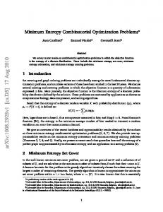
Figure 11: The subdivision of the point set into constant-size subsets of P and ρ(P ) ≤ 5b n−2 12 c + 4 can be found in O(n log n) time. Proof.
The proof of Theorem 3.6 and the discussion in Section 3.3 yield an algo-
rithm for computing a polygonalization with at most based on the subdivision of the set size
13
R
and
L,
and the edge
De�ne
t0l , Rl0 ,
and
re�ex vertices,
into (not necessarily disjoint) subsets of
(apart from one subset of size at most
M = b(n − 2)/12c. sets
S
5b n−2 12 c + 4
L0l ,
13).
Set
t00 = q , L00 = S ,
recursively, to be the point
pt0l−1 , 1 ≤ l ≤ M .
Once the points
stated number of re�ex vertices: For each time) a polygonalization
t0l
Pl
Rl0 ,
of
1≤l≤M
such that
Pl
and the sets
Rl0
we get a polygonal chain
L0M = {p, t0M }, P
P
starting at
have been
S
time a polygonalization
pt0M
PM +1
four re�ex vertices (note that
and
of
L0M
pq .
with the
and has
from every polygon
and ending at
t0M .
If
Pl ,
|L0M | = 2, S
by con-
Otherwise, one can compute in constant
containing the edge
|L0M | ≤ 13).
and concatenating the resulting chain to
S
t0l t0l−1
t0l t0l−1
then we obtain the desired polygonalization of
the edges
polygonalization of
t00 = q
L0l−1
we computed (in constant
contains the edge
at most four re�ex vertices. By removing the edge
catenating to
and the
respectively, guaranteed by applying Lemma 3.3 on the set
computed it is easy to compute in linear time the polygonalization of
that is
t
and
P
pt0M
and having at most
By removing the edge and the edge
pq
pt0M
from
PM +1
we obtain the desired
(see Figure 11 for an illustration).
Therefore, it remains to depict the details of the subdivision described in
47
Lemma 3.3. Algorithm 3.4 describes the implementation of this subdivision.
It
uses the dynamic planar convex hull of Brodal and Jacob [13]. This data structure, denoted by
DCH,
maintains the convex hull of a set of points and supports,
among other things, the following operations:
• DCH.INSERT(v ):
insert a new point
• DCH.DELETE(v ):
remove the point
• DCH.CCW(v ): point
v,
v;
v;
and
get the counter-clockwise neighbor in the convex hull of the
where
v
is a vertex of the convex hull;
Insertions and deletions are performed in
O(log n)
O(log n)
counter-clockwise neighbor query takes
amortized time, while the
worst-case time.
Next, we explain Algorithm 3.4, using the notation of Lemma 3.3. The algorithm begins by removing the vertex
q
we remove CCW(t1 ) repeatedly at most
k−2
(lines 15�23). If
Otherwise, by deleting
∠t2 pq
Now, CCW(p) is
t1 .
Then,
times while it is to the right of
e1
k − 2 times CCW(t1 ) was to the right of e1 , then all those points
that were removed along with
est angle
(line 5).
t1
t1
constitute the set
R,
with
(line 5), CCW(p) is the point
among the points to the left of
e1 .
t2
t = t1
(lines 24�27).
that forms the small-
The algorithm proceeds by
re-inserting all the points that were deleted in the previous iteration and are to the left of the line determined by
p
and
t2
(lines 9�12). This step is performed
since it is possible that these points will not be among the set of points creating the
(k − 2)nd
smallest angles
right of the line through
p
and
t2
p 0 ti q
(whereas the points that are to the
must be in this set, and thus, remain in
Next, we remove CCW(t2 ) repeatedly (as long as it is to the right of time
k − 1 − |R|
to the right of
times (lines 15�23). As before, if
e2 ,
p0 ∈ S 2
k − 1 − |R|
e2 ),
R). this
times CCW(t2 ) was
then we are done. Otherwise, we proceed to the next point
For the same arguments used to claim that Lemma 3.3 it follows that the size of
R
|Si | > |Si−1 |
t3 .
in the proof of
at, say, line 24 grows along the iterations
48
A set of n points S ; DCH(S ); p, q ∈ S s.t. pq is a boundary edge of CH (S); an integer k > 2 Ensure: The set R and the point t as described in Lemma 3.3. R ← ∅; i ← 0; ti ← q ;
Require:
|R| < k do DCH.DELETE(ti ); R ← R ∪ {ti }; i ← i + 1; ti ← DCH.CCW(p); for all {r ∈ R : r is to the left of the line through p and ti } R ← R \ {r}; DCH.INSERT(r);
while
do
end for
ei ← the line through q and ti ; m ← (k − 1 − |R|); /* The number of points missing in R */ for j = 1 to m do s ← DCH.CCW(ti ); if s is to the right of ei then DCH.DELETE(s); R ← R ∪ {s}; else
quit the for-loop; end if end for if
s is to the right of ei then R ← R ∪ {ti }; /* |R| = k */ t ← ti ;
end if end while
Algorithm 1: Generating the subdivision of Lemma 3.3
49
of the main loop (lines 4�28). Therefore, the main loop is executed
O(k)
and thus, the run-time of the procedure described in Algorithm 3.4 is amortized time. The number of times this procedure is executed is the overall run-time, including the initialization of case
k = 13,
the run-time is
DCH,
is
times,
O(k 2 log n)
O(n/k).
O(nk log n).
Thus,
As in our
O(n log n).
3.5 Discussion and Open Problems We showed that for every set is a polygonalization of
S
S
of
n
points in general position in the plane there
with at most
polygonalization can be found in
5b n−2 12 c + 4
O(n log n)
time.
re�ex vertices, and such a
The basic idea of the proof
is that by Lemma 3.3 we can subdivide
S
a stronger result on each of these parts.
It would be interesting to �nd other
into some �xed-size parts and use
applications of the subdivision suggested in Lemma 3.3. Recently Günter Rote informed us that this kind of subdivision was utilized in papers about straight line embeddings of outerplanar graphs (see [25], [14], [10]). Moreover, for achieving the same subdivision they use a simpler algorithm which - using the structure - works in amortized time
DCH
data
O(k log n), whereas ours works in O(k 2 log n)
amortized time. Yet, in our application
k
is a small constant, thus utilizing their
algorithm only simpli�es things, does not improve the result signi�cantly. Conjecture 3.4 in [9] states that
ρ(n) = b n4 c.
Introduction, considering the values for
As already mentioned in the
ρ(n) in Tables 2 and 5 the conjecture has
to be modi�ed to
Conjecture 3.11.
b n4 c ≤ ρ(n) ≤ d n4 e.
It is a challenging open problem to determine the structure of sets maximizing the re�exivity for �xed cardinality. On the one hand we have the sets used in [9] to provide the bound of
ρ(n) ≥ b n4 c,
boundary of the convex hull.
which have half of their vertices on the
This so-called double circle con�guration is also
50
conjectured to minimize the number of triangulations [4], and therefore seems to be a promising extremal example, supporting Conjecture 3.11. On the other hand all maximizing examples for be that for larger cardinality than
ρ(n),
ρ¯(11) have a triangular convex hull, so it could
ρ¯(n)
is more than a constant additive factor larger
contradicting Conjecture 3.12.
It would be interesting to bound
Conjecture 3.12.
ρ¯(n)
in terms of
ρ(n).
There is a constant c0 such that ρ¯(n) ≤ ρ(n) + c0 . ρ¯(S) ≤ ρ(S) + O(1) for any set S
Note that the stronger statement that
might
also hold. Conjecture 3.12, if true, would mean that it is possible (although not necessarily practical) to get arbitrarily close to the best possible linear upper bound by checking only �nitely many small cases. jecture holds and there is
k = k(�)
c
is a constant such that
such that if we verify that
ρ(n) ≤ (c + �)n + O(1).
Indeed,
k
In other words, suppose the con-
ρ(n) ≤ cn. ρ(k) ≤ ck ,
Then, for any
then for
large enough such that
n>k
ck+c0 +1 k−1
� > 0
we have
≤ (c + �)
holds, would do. Moreover, the discussion above is still valid if we replace Conjecture 3.12 by some function
f (n)
such that
Following the notation of [9], a
be added to
S
in
f (n) ∈ o(n).
Conjecture 3.12 is true when we consider re�exivity in the presence of
points.
c0
Steiner point
is a point
q∈ / S
Steiner
that may
in order to improve some structure. For example, we de�ne the
Steiner re�exivity of S , ρ0 (S), to be the minimum number of re�ex vertices of any simple polygon with vertex set
V ⊇ S.
Similarly,
ρ0 (n) = max|S|=n ρ0 (S).
The
(stronger statement) of Conjecture 3.12 can be easily proved if we allow Steiner points.
Lemma 3.13.
Let S be a set of n points and let pq be a boundary edge of CH (S).
Then, there are points p0 , q 0 (inside CH (S)) such that S ∪ {p0 , q 0 } has a polygonalization containing the edge pq and having at most ρ(S) + 1 re�ex vertices.
51
q2
q2
p1
p1 q1
q1 p
p
′
q′
p
q
q
(a)
(b)
Figure 12: An illustration for the proof of Lemma 3.13 Proof.
and the remaining points be a polygonalization of that
P
S \ {p, q}
S,
such that
P
p1
pq
and
q1 q q2
P0
of a set
and
pq .
V ⊃S
q,
is left to
q.
P
Let
We show
such that
P0
ρ(P 0 ) ≤ ρ(P ) + 1.
counter-clockwise and clockwise neighbors of
the chain
p
does not contain the edge
be the counter-clockwise neighbor of
to the right and above
p
is horizontal,
are above the line through
can be modi�ed into a polygonalization
contains the edge Let
pq
We assume, w.l.o.g., that the �xed edge
p, and q 0
with the chain
q
p
in
in
P,
P,
and let
and the edge
one obtains the desired polygonalization
P0
and
respectively. Fix
slightly to the left and above
q1 q 0 q2 ,
q1
p p1
q.
q2 p0
be the
slightly
Now by replacing
with the chain
p q p0 p1 ,
(see Figure 12 for an illustration).
Note that the only re�ex vertex that might be introduced in these steps is
p0 .
As before, this implies that we can get arbitrarily close to any linear upper bound on
ρ0 (n) by checking only �nitely many small cases.
Note that it is impor-
tant here that the Steiner points we add lie inside the convex hull of the original set of points. Adding a (Steiner) point to a set of points might result in a set of points whose re�exivity is smaller than this of the original set (see [9] for examples). However, we are con�dent, although we were not able to prove, that for every set of points one can add some point that will not reduce the re�exivity. This would imply
Conjecture 3.14.
ρ(n + 1) ≥ ρ(n)
52
A similar statement should hold for restricted re�exivity.
Conjecture 3.15.
ρ¯(n + 1) ≥ ρ¯(n)
If this conjecture is true, then the last inequality of Corollary 3.7 always holds.
53
4 Polychromatic colorings of rectangular partitions First we regard the problem of polychromatic colorings and rectangle-respecting colorings for rectangular partitions, and then for guillotine-partitions in higher dimensions.
4.1 Polychromatic colorings of planar rectangular partitions Polychromatic
4-colorings
We start with the de�nition of [44] about
4-graphs,
of rectangular partitions
r-graphs,
then state the conjecture of Seymour
which was proved recently by Guenin [26]. Note that this
theorem implies the four-color theorem. An
r-graph is an r-regular (multi)-graph
G on an even number of vertices with the property that every edge-cut separating V (G)
into two sets of odd cardinality has size at least
Theorem 4.1 (Guenin).
r.
Every planar 4-graph is 4-edge-colorable.
In the rest of this section we will prove that this theorem implies the following.
Theorem 4.2.
There is a strong rectangle-respecting 4-coloring of any rectangu-
lar partition. Proof.
Take an arbitrary rectangular partition. We will give a strong rectangle-
respecting
4-coloring
of it.
First, if it has an even number of rectangles then
add one rectangle to the left side of the partition for example. Coloring this new partition (which has an odd number of rectangles) also gives a coloring of the original one. Now we contruct the planar graph on which we can apply Theorem 4.1. First put a point in the center of all the rectangles. Connect two such points with an edge whenever the corresponding rectangles have a common corner. Draw
54
p
p
P (W ′ )
(a) The graph constructed from the rect-
(b) The edges of the edge-cut guaranteed
angular partition
by the proof
Figure 13: Example for the proof of Theorem 4.2 this edge in the plane by two segments, one going from the center point of the �rst rectangle to the common corner and the second going from here to the center point of the other. This way we clearly built a planar graph on an odd number of points. Further, add a point
c
p
outside the partitioned rectangle. For each corner
of the partitioned rectangle take the rectangle
a corner. Then connect
p
to the center
r
of
R,
R
in the partition that has
c
as
with a polygon going through
c
as well. This can easily be done for all four corners of the partitioned rectangle in a way that the �nal graph is still a plane graph. Now our graph has an even number of points. The new point
p
corresponding to a rectangle has
4
each of its corners.
4-regular.
has
4
outgoing edges and an arbitrary point
outgoing edges as well, one going through
Thus, this graph
G
has an even number of points and is
For an example see Figure 13(a). Note that the resulting graph can be
a multigraph and that we needed that no
4
rectangles meet at a common corner.
To be able to apply Theorem 4.1 we only need to prove that every edge-cut separating
V (G)
into two sets of odd cardinality has size at least
arbitrary cut of this kind. The two point sets of the cut are
p
is in
V \W.
Take a maximal connected component
55
W0
of
W W.
and
r.
Take an
V \W
where
If two points are
1
1
3
2
4
3
2
4
4
1
3
4
1
3
(a)
(b)
Figure 14: The partition T and two di�erent colorings connected in the graph then the corresponding rectangles have a common segment on their borders, thus the rectangles corresponding to whose every edge is horizontal or vertical.
Thus,
W0
W0
form a polygon
P (W 0 )
has at least four convex
corners. It is enough to prove that the edge corresponding to such a corner
c
is
part of the edge-cut. Indeed one end of such an edge is the point corresponding to the rectangle in
P (W 0 ) (and so it is in W ) whose corner is c and the other end
is a point corresponding to a rectangle outside
W0 G
this cannot be in
W.
P (W 0 )
and by the maximality of
For an example see Figure 13(b), where the
corresponding to the convex corners of
Now, applying Theorem 4.1 we get a
P (W 0 )
5
edges of
are solid, the rest are dotted.
4-coloring of the edges.
Give the same colors
for the corresponding corners of the partition, this is clearly a strong rectanglerespecting
4-coloring
Polychromatic
as we needed.
4-colorings
of general rectangular partitions
In the rest of this section we deal with general rectangular partitions, and so for simplicity, in the remainder of this section we will use the terms partition and general partition interchangeably. The previous theorem does not hold for general rectangular partitions as it was mentioned in the Introduction. that even a polychromatic
Now we prove
4-coloring does not always exist for general partitions.
56
G1
G2
G3
G4
Figure 15: The partition Q and subpartitions G1 , G2 , G3 , G4 4-coloring
We want to �nd a
of a given partition such that for any rectangle all
four colors appear on the vertices on the boundary of that rectangle. Denote by
G
the
3×3
grid (i.e. four squares) and by
T
the partition obtained from a
3×3
grid by merging the upper two squares (see Figure 14). When referring to a of the partition
G
or
T
side
we mean the set of vertices on the corresponding vertical
or horizontal boundary of the partition (e.g. left, right, upper, lower). We begin with some simple observations.
Observation 4.3.
If a weak rectangle-respecting 4-coloring of the 3 × 3 grid G
assigns three colors to some side of G , then the same three colors appear on the opposite side of G .
Observation 4.4.
A weak rectangle-respecting 4-coloring of a 3×3 grid G cannot
simultaneously assign three colors to the left (or right) and lower (or upper) sides.
Observation 4.5.
A weak rectangle-respecting 4-coloring of T assigns three col-
ors to the left side or right side of T . Let us de�ne a new partition
Q
(See Figure 14.)
as follows: start with a
7×7
grid, �rst merge
the four central squares, then for each side of this new center square merge the two smaller squares adjacent to that side. In this way we obtain a partition that contains four copies of
G
and four rotations of
57
T.
See Figure 15 for an illustration
Figure 16: Proof of Theorem 1.14, C , the counterexample of
Q.
Claim 4.6.
Let G1 (resp. G2 ) be the 3 × 3 grid in the upper-left (resp. upper-
right) corner of Q. A weak rectangle-respecting 4-coloring of the partition Q must assign three colors to either the upper side of G1 or the upper side of G2 . Proof.
G3
Let
corner of
Q
G1
G4 )
be the
3×3
grid in the lower-left (resp. lower-right)
(see Figure 15). Assume that neither the upper side of
upper side of side of
(resp.
G2
G1
nor the
are assigned three colors. By Observation 4.3 neither the lower
nor the lower side of
the upper sides of
G3
and
vation 4.4 the right side of
G2
are assigned three colors. By Observation 4.5
G4
are each assigned three colors. Finally, by Obser-
G3
has exactly two colors and the left side of
G4
has
exactly two color. However, now we have colored the right and left sides of the partition
T
on the bottom of
Q
in a way that contradicts Observation 4.5.
Note that a similar claim holds for each side of
Q
as we can simply rotate
and follow the proof of Claim 4.6. Let us de�ne a new partition with a
C
Q
as follows: start
3 × 3 grid and embed a 7 × 7 grid in the upper-right square, a copy of Q in
the upper-left square and a copy of
Q in the lower-right square.
an illustration. We will show that partition
58
C
See Figure 16 for
has no weak rectangle-respecting
4-coloring
thus proving Theorem 1.14.
Proof of Theorem 1.14. lower-right copy of
Q.
rotation of
Q1
Q1
be the upper-left copy of
By applying Claim 4.6 to
on the lower side of the
−90o
Let
7×7
we �nd
Q2
we �nd
Q
and let
Q2
be the
3 consecutive vertices
grid with three colors. By applying Claim 4.6 to a
3
consecutive vertices on the right side of the
7×7
grid with three colors. By application of Observation 4.3 it is easy to see that we can �nd a
3 × 3 grid
in the
7 × 7 grid
that has three colors on both the lower side
and right side. This contradicts Observation 4.4.
The elements of this construction are the main building parts to prove that it is
N P -complete to decide if a general rectangular partition admits a polychromatic 4-coloring. respecting
We know several smaller partitions that have no weak rectangle-
4-coloring,
the smallest known construction has
the counterexample presented here has
Weak rectangle-respecting
3-
124
and
65
vertices (whereas
vertices).
5-colorings
of general rectangu-
lar partitions
In this part we want to prove that any partition admits a weak rectangle-respecting
3-
and
5-coloring.
Consider a partition in the coordinate plane. smallest to largest
x
Let us arrange vertices from
coordinate then from largest to smallest
y
coordinate i.e.
from left to right then top to bottom. We refer to this ordering as the
order
upper-left
of the vertices. Two vertices are neighbors if there is a segment between
them containing no other vertex.
Proposition 4.7.
Every general partition admits a weak rectangle-respecting 3-
coloring (i.e. a polychromatic 3-coloring). Proof. any
v
Let
R be a partition.
We will greedily
3-color the vertices of R.
Note that
vertex has at most one neighbor above it and at most one left to it (the
59
neighbor with smaller
x-coordinate
and the neighbor with larger
y -coordinate).
We will always maintain a coloring such that any vertex has a di�erent color from these at most
2
neighbors of it.
R
Next, consider the vertices of
arranged in upper-left order.
rectangle we will ensure that it has at least
3
For a given
colors on its boundary in the step
when we consider its lower right corner. Let
v
be the pending vertex to be colored. If
colored neighbor
w
then color
v
previously-colored neighbors, say of a common rectangle and If
x
and
y
v
v
has exactly one previously-
with a color di�erent from
x
and
y,
then
v, x
and
r
If
v
has two
are on the boundary
is the bottom-right corner of this rectangle.
are colored with di�erent colors then color
Thus, the rectangle
y
w.
containing
v, x
and
y
will have
3
v
with the third color.
di�erent colors on its
boundary as we wanted. If
y
and
x
are colored with the same color then we will color
di�erent from that used on already colored neighbor neighbor of
x
and
y,
x
and
y.
w.
These two points must have at least one
By induction
w
with the color unused by
x
in which case it is the top left corner of
Thus, rectangle
with a color
w on the boundary of rectangle r (this may be a common
x
has di�erent color from the color of and
v
r
will have
In this way every rectangle of
3
R
and
y.
Color
v
r).
di�erent colors on its boundary as needed.
will include three di�erent colors among the
vertices on its boundary.
Proposition 4.8.
Every general partition admits a weak rectangle-respecting 5-
coloring. Proof. any
v
Let
R be a partition.
We will greedily
5-color the vertices of R.
Note that
vertex has at most one neighbor above it and at most one left to it (the
neighbor with smaller
x-coordinate
and the neighbor with larger
y -coordinate).
Again, we will always maintain a coloring such that any vertex has a di�erent
60
1
2
3
2 u
1
3
4 v
2
A 4
B
1 w
Figure 17: w cannot be colored to 1, 2, 3 because of A, neither to 4 because of v in B color from these at most
2
neighbors of it.
Next, consider the vertices of
B
R arranged in upper-left order.
we will ensure that it has at least
we consider the vertex so we color
v
v
2
colors on its boundary in the step when
right to its top left vertex
di�erently from
u).
u (v
We will ensure that
u
below
ensure that
u
(we color it di�erently from
B
has at least
its lower right corner of
B,
we color
x
x
4
u
and
u's
and
B
its boundary in the step when we consider the vertex of
For a given rectangle
u
are neighbors and
has at least
w
3
colors on
which is the neighbor
right neighbor
v ).
We will
colors on its boundary in the step when we consider
(in case there are only
3
colors present on the boundary
di�erently from these).
Following these rules we will get a needed coloring. Thus, it is enough to prove that when coloring a vertex there are at most
5
4 colors we need to avoid, thus using
colors we can color greedily all the vertices. If a vertex does not need to ensure
a third or fourth color on some rectangle, then we need to color it di�erently only from its left and upper neighbor, that is we need to avoid at most a vertex
w
ensures a third color on some
B
2
colors. If
(but it does not need to ensure a
fourth color on any of the rectangles) then when coloring it we need to avoid the color of its left neighbor (if it exists), its upper neighbor of
u,
thus at most
rectangle
A,
3
u and the right neighbor
colors. If a vertex needs to ensure a fourth color on some
then we need to avoid at most
61
3
colors (including the colors of its
left and upper neighbor). If at the same time this vertex ensures a third color on some rectangle
B,
then one more color needs to be avoided (the color of the
right neighbor of its upper neighbor). Together this is again at most
4
colors to
be avoided (see Figure 17 for an illustration of this worst case).
Strong rectangle-respecting
2-
and
6-colorings
of general rectan-
gular partitions
In this section we either want to �nd the minimal number number that
k≥4
or the maximal
k < 4 of colors such that every partition can be colored with k colors such
min{k, 4}
colors appear on the
4
corners of every rectangle of the partition.
First we show the existence of a strong rectangle-respecting
Proposition 4.9.
2-coloring.
Every general partition admits a strong rectangle-respecting
2-coloring.
Proof.
For a given partition
exactly two colors.
Let
above and to the left of
v
v v
R
let us color the vertices in upper-left order with
be the pending vertex to be colored.
Only vertices
are already colored. Thus, only the rectangle that has
in its lower right corner may have three previously colored corners. If the three
previously colored corners have the same color, then choose the other color for Otherwise choose any color for
v.
v.
After coloring all vertices in this way clearly
no rectangle will have a single color among its four corners.
A simple greedy algorithm similar to those used for weak rectangle-respecting
5-colorings shows that for a partition there is always a strong rectangle-respecting 7-coloring. respecting
We present a proof that every partition has a strong rectangle-
6-coloring.
Proposition 4.10.
Every general partition admits a strong rectangle-respecting
6-coloring.
62
y x
Figure 18: orientation of edge xy Proof. xy
For a given partition
is an edge of
G
R, let G be the graph with the vertex set of R, where
if and only if
x
and
y
are corners of the same rectangle in
Clearly, the proposition is proved if we can �nd a proper
6-coloring
of
G.
R.
First
we will color the vertices where four rectangles meet. We use a greedy algorithm with the vertices in upper-left order. Every vertex has at most four previously colored neighbors, hence six colors are (more than) enough to properly color such vertices. Denote by
W
the set of all so-far uncolored vertices of
R.
A vertex in
W
is
the corner of at most two rectangles, thus has degree at most six in the graph
G.
Let
W0 ⊂ W
be the set of vertices of degree
6.
A vertex
x ∈ W0
must be the
corner of exactly two rectangles that do not share a second corner. Hence two neighbors lying on a common line segment starting from Denote the closer one of these two neighbors by
y.
in
G
from
vertices in
x
W0
to
y.
W0
vertex with indegree zero. The vertex
with indegree zero.
from
must be the
direct the edge
y
to
x.
Thus all
W 0.
Let
x ∈ W0
be a
x has outdegree one, so x has an uncolored
neighbor, thus there is an available color for
x
y
have outdegree exactly one.
Let us �rst color the vertices of
remove
x and y
Note that this procedure will never direct
has
(see Figure 18).
Observe that
corner of exactly two rectangles. Now for every such pair
xy
x
x
x.
Color
x with an available color and
Repeat this step until no vertex with indegree zero remains
63
in
W 0.
Now every vertex in
the remaining vertices of on a directed cycle in
W0
W0
W0
has outdegree and indegree equal to
1.
Therefore
can be partitioned into directed cycles. The vertices
have at most
4
previously colored neighbors, so each
vertex has a list of at least two available colors. If we examine these cycles in
R it is clear that the edges must alternate between
vertical and horizontal orientation. Thus these directed cycles are of even length. The list-chromatic number of an even cycle is properly. Now all vertices in in
G
are the vertices of
W0
W − W 0.
2,
hence each cycle can be colored
are colored. The remaining uncolored vertices These vertices have degree at most
5
and thus
all have an available color.
4.2 Polychromatic colorings of n-dimensional guillotinepartitions In this section our aim is to prove the following theorem.
Theorem 4.11.
There is a strong hyperbox-respecting coloring of any n-dimen-
sional guillotine-partition. Note that the theorem is about partitions where no more than are allowed to meet at a common corner.
2
hyperboxes
First we start with some de�nitions
to be able to phrase the theorem we will actually prove, implying Theorem 4.11. We begin by introducing some notations.
y, z, a, b, c, d,
etc. always refer to some
two such vectors (denoted simply by mod
e1 .
2. A
The
face
(0, 0, . . . , 0)
From now on
n-long
0-1 vector. We de�ne the sum of
+) as summing independently all coordinates
vector is denoted by
is always an (n
x = (x1 , x2 , . . . , xn ),
0
− 1)-dimensional
and the vector
(1, 0, 0, . . . , 0)
face of a hyperbox.
by
Fix now the
unit hyperbox, the 0-1 vectors being its corners. First we de�ne the forthcoming notions only for this hyperbox. For some �xed
x 6= 0
being the function on the set of corners for which
64
we de�ne the
Rx (y) = x + y
re�ection Rx
for all
y.
It is
indeed a re�ection on an of
1's
x.
in
Observe that
(n − k)-dimensional Rx (Rx (y)) = y
hyper-plane where
for any
is the number
y.
We say that a coloring of the corners of the hyperbox is an two corners
k
Rx -coloring (x 6= 0) if
y and z have the same colors if and only if Rx (y) = z (or equivalently
Rx (z) = y).
Observe that such a coloring will have
2n−1 di�erent colors appearing
on the corners of the hyperbox, each occuring twice. Further, we say that the coloring of the corners is an that for any
x,
R0 -coloring if all corners are colored di�erently.
permuting the colors of an
Rx -coloring gives another Rx -coloring.
Given now an arbitrary axis-parallel hyperbox
B,
the unit hypercube can be
uniquely scaled (with positive coe�cients) and translated into transformation by
C
(depends on
B ).
The function
C
the corners of the unit hypercube) onto the corners of of
B
are the set of
corners).
C(y)'s (B
By this bijection an
and
y
Note
given,
Rx -coloring
C(y)
B.
Denote this
maps the 0-1 vectors (i.e.
B,
thus the set of corners
uniquely denotes one of
B 's
can be analogously de�ned on this
hyperbox, thus on an arbitrary hyperbox. From now on we will always restrict ourselves to these kinds of colorings. Further, when we speak about a coloring of some partitioned hyperbox then it will be always a hyperbox-respecting coloring.
If any pair of such colorings could be
put together along any axes to form another such coloring then it would already imply a recursive proof for the main theorem. As this is not the case we have to be more precise about our freedom of how to color a partition, making necessary to de�ne sets of such colorings. For any
x 6= 0 Sx
product of for all
x
and
y ∈ Sx
which is an
y
mod
2). S0
Ry 's for which x · y = 1 (the scalar
is the one element set of
R0 .
If for some
x 6= 0
the hyperbox partition has a strong hyperbox-respecting coloring
Ry -coloring
be colored by the which is an
is de�ned as the union of all
on its corners, we say that the hyperbox partition can
color-range Sx .
R0 -coloring
If it has a strong hyperbox-respecting coloring
on its corners, we say that the hyperbox partiton can be
65
colored by the (one element)
color-range S0 .
We will prove the following theorem, which implies Theorem 4.11.
Theorem 4.12.
Any n-dimensional guillotine-partition can be colored by some
color-range. Proof.
We proceed by induction on the number of guillotine-cuts of the partiton.
The corners of a hyperbox containing only one basic hyperbox (i.e. the partition has 0 cuts) can be colored trivially with all di�erent colors, thus colorable by color-range
S0 .
into two hyperboxes
B1
and
B2
We need to prove that there exists a
be colored by
Sz .
splitting it
with smaller number of cuts in them. Thus, by
induction they can be colored by some color-ranges
y.
B
In the general step we take a cut of the hyperbox
z
Sx
and
Sy
for some
x
and
for which our hyperbox partition can
First we prove this for the case when the cut is orthogonal
to the �rst axis. Finally, we will prove that as the de�nition of
R's
and
S 's
is
symmetrical on every pair of axes, the claim follows for any kind of cut. We regard the �rst axis (the one which corresponds to the �rst coordinate of points) as the usual perbox etc.) is
left
x-axis,
and so we can say that an object (corner, face, hy-
from another if its �rst coordinates are smaller or equal than
the other's (B1 is left from
B2
for example). Similarly we can say
right
when its
coordinates are bigger or equal than the other's. We always do the following. Take an ing of an
B1
which is an
Rb -coloring
Ra -coloring
R a ∈ Sx
and
Rb ∈ Sy
and take a color-
on its corners and a coloring of
B2
which is
on its corners by induction such that the colors of the corners
which should �t together (the right face of
B1
and the left face of
B2 )
have the
same colors at the corners which will be identi�ed. This is not always possible but when it is, it gives a coloring of on the right face of
B2
B
(the corners on the left face of
are the corners of
B ).
B1
and
Note that we can permute the
colors on the two hyperboxes in order to achieve such a �t of the colors. Clearly, the resulting coloring of
B
is a hyperbox-respecting coloring by induction.
66
If
4
2
4
5
3
2
5
3
6
4
1 6
4
3
2
5
3
2 1
6
4
3
1
6
4
1
5
3
Figure 19: Example to Lemma 4.13(c): R010 · R010 →R010 the resulting coloring can be an write
Ra · Rb →Rc .
de�nition of
→
Rc -coloring
on the corners for some
c
then we
See Figure 19 and 20 for examples for 3 dimensions.
The
is good as the existence of such a �t depends only on the color
of the corners. Observe that this operation is not commutative by de�nition and can hold for more than one
c
and has the hidden parameter that we put them
together along the �rst axis (i.e. the two partitions are put together by the face which is orthogonal to the �rst axis). As we remarked earlier, if for any there would be a
c
with
Ra · Rb →Rc
a
and
b
then it would be enough to prove the main
theorem by induction without de�ning color-ranges. As this is not the case we need to deal with color-ranges and de�ne the function We write
Sx · Sy →Sz
if
∀Rc ∈ Sz ∃Ra ∈ Sx
and
R b ∈ Sy
Clearly, we need to prove that there exists such a that
Sx · Sy →Sz .
→
z
on them as well. such that
Ra · Rb →Rc .
for any choice of
x
and
y
Lemma 4.14 states this. For the proof of this lemma we will
�rst need to prove Lemma 4.13 about the behaviour of
→
for
R's.
Finally, we need to prove that we can put together color-ranges along any axis. One can argue that we can obviously do that as the de�nition of color-ranges is symmetrical on any pair of coordinates and because of that analogs of Lemma 4.13 and Lemma 4.14 are true for an arbitrary axis. For a more rigorous argument see Lemma 5.7 and its proof in the Appendix.
Lemma 4.13 (�tting together colorings).
For a, b, c 6= 0 we have
(a) R0 · R0 →Rc , if the �rst coordinate of c is 1, (b) Ra · R0 →R0 and R0 · Ra →R0 , if the �rst coordinate of a is 1,
67
2
4
2
1
2
4
3
1
2
3 3
4
3
1
4
2
1 4
2
1
2
1
3
3
4
1
4
3
Figure 20: Example to Lemma 4.13(d): R110 · R101 →R111 (c) Ra · Ra →Ra , if the �rst coordinate of a is 0, (d) Ra · Rb →Rc , if the �rst coordinate of a and b is 1 and c = a + b + e1 . Proof.
(a) Take an arbitrary
c
with its �rst coordinate being 1.
For an
Rc -
coloring each color appearing on the corners of the hyperbox appears once on its left and once on its right face. We want to �t together two an
Rc -coloring.
Take an arbitrary
R0 -coloring
B1 .
of
R0 -colorings
Take an
to have
R0 -coloring
of
B2
and permute its colors such that the corners on its left face �t together with the
B1 .
corners on the right face of
Now the set of colors on the right face of
the same set of colors as on the left face of these colors on
we can get an
Ra -coloring
(b) Take an
B2
B2
of
B1
B1 .
Rc -coloring
and an
on
B. of
B2 ,
permute the colors on
such that the needed faces �t together. This can be done as
colors appear as on its right face, on its corners, thus it is an
B
As on
B1 's
of
B.
Ra
does not have
left face the same set of
has all the colors of
R0 -coloring
is
After a possible permutation of
R0 -coloring
a color appearing twice on its right face.
B2
B2 's
coloring appearing
The proof for the other claim is
similar. (c) Take an
Ra -coloring of B1 .
Take an
Ra -coloring of B2
and permute the colors
on it such that the corners on its left face �t together with the corners on the right face of
B1
and on its right face all colors are di�erent from the ones we
used to color the corners of the �rst coordinate of
a
B1 .
This can be done as both are
Ra -colorings where
is 0, so on the common face the same pair of corners
need to have the same color. Similarly, we see that these �t together to form an
68
Ra -coloring
of
(d) Take an
B.
For an illustration for 3 dimensions see Figure 19.
Ra -coloring
of
B1 .
Take an
Rb -coloring
of
B2
and permute again
the colors such that the corners on its left face �t together with the corners on
B1 .
the right face of
This can be done as the corners on the right face of
have di�erent colors and this is what we need on the left face of
Rb
coloring (as the �rst coordinate of
the resulting coloring of
e1
B
Rc
is an
coloring with
coloring of
B1
Now it is enough to see that
c = a + b + e1
B2 's
B1 ,
d
(recall that
has �rst coordinate
Rb -coloring
of
B2
the corner
C(d + a + e1 + b)
the same color. This is also the
B
C(d + a).
and so it is �tted together with the corner
left face. By the
any corner of
(thus
its pair (the corner with the same color) is
the right face of on
C(d)
all
to make an
is the vector with all-0 coordinates except the �rst coordinate being
an arbitrary corner on its left face,
B2
a and b is 1).
B2
B1
1).
0).
Take
In the
This is on
C(d + a + e1 )
C(d + a + e1 + b)
corner of
B.
of
has
This holds for
on its left side and symmetrically on its right side as well, and so
this is indeed an
Rc -coloring of B .
For an illustration for 3 dimensions see Figure
20.
Lemma 4.14 (�tting together color-ranges).
For x, x0 , y 6= 0 we have
(a) S0 · S0 →Se1 , (b) Sx · S0 →S0 and S0 · Sx →S0 , (c) Sx · Sy →Se1 , if x and y di�er somewhere which is not the �rst coordinate, (d) Sx · Sx →Sx0 , if x0 is the same as x with the possible exception at the �rst coordinate, which is 1 in x0 . (e) Sx ·Sx0 →Sx and Sx0 ·Sx →Sx , if x0 is the same as x except at the �rst coordinate, which is 0 in x and 1 in x0 . Proof. Sx
Let us recall �rst that
S0
is de�ned as the union of all
is the one element set of
Ry
for which
69
x · y = 1.
R0
and for any
x 6= 0
(a) by Lemma 4.13(a) (b) In
Sx (x 6= 0)
Lemma 4.13(b)
R0 · R0 →Rc
there is always an
Ra · R0 →R0 .
R b ∈ Sy
such that
Suppose
x
l
coordinates
y
Ra
c · e1 = 1.
Rc ∈ Se1 (c · e1 = 1)
k ∈ / X
k th
di�er in the
where
and
there is an
xl = 1, and Y
k ∈ Y.
6= 1).
coordinate (k
the set of coordinates
a
The �rst coordinate of
and
c
except one (this is the �rst if
1 ∈ X,
coordinates of
b
such that
a
not in
X
such that
R a ∈ Sx .
al + bl = cl
such that
b · y = 1,
and
l
b
where
al + bl = cl
as the set of
yl = 1.
We want
and so we can suppose
a
a + b + e1 = c a
being in
b
and
to be able
X
all zero
for all
Now de�ne the coordinates of
l ∈ X.
De�ne the rest of the
this can be done as we can choose the
R b ∈ Sy
coordinate as we want. Thus, of
By
some other otherwise), thus by any choice
of the other coordinates we will have
X \ {1}
X
De�ne
to apply Lemma 4.13(d). First de�ne the coordinates of
being in
R a ∈ Sx
is 1, so we choose
having the �rst coordinate 1 as well. We need that
b
1.
is
Ra · Rb →Rc .
to apply Lemma 4.13(d) which is symmetric on that
a
where the �rst coordinate of
The proof for the other claim is similar.
(c) We need to prove that for any
and
for any
k th
as well. Finally, choose the coordinates
for all
l∈ / X.
This way
a + b + e1 = c
as
needed. (d) We need to prove that for any such that
Rc ∈ Sx0
there is an
with �rst coordinate
c
holds.
R b ∈ Sx
Choose
x
is 1 and so
x0 = x.
For a
c
0 by Lemma 4.13(c) we have Rc ·Rc →Rc , all in Sx as needed.
with �rst coordinate
R a ∈ Sx .
and
Ra · Rb →Rc .
First we prove the case when the �rst coordinate of
For a
R a ∈ Sx
1
take an arbitrary
a
with �rst coordinate
1
and
b such that a+b+e1 = c and so by Lemma 4.13(d) Ra ·Rb →Rc
We need that
Rb
is in
Sx ,
which is true as
b · x = (a + c + e1 ) · x =
1 + 1 + 1 = 1. Now we prove the case when the �rst coordinate of
x is 0 and so x0 = x+e1 .
For a
c with �rst coordinate 0 by Lemma 4.13(c) we have Rc ·Rc →Rc , all in Sx and in Sx0
70
too (as for such a arbitrary
c we have c·x = c·x0 = 1).
For a
a with �rst coordinate 1 and Ra ∈ Sx .
and so by Lemma 4.13(d)
Ra · Rb →Rc
c with �rst coordinate 1 take an
Choose
b such that a+b+e1 = c
holds. We need that
Rb
is in
Sx ,
which is
true as
c · x0 = 1, c · e1 = 1 and so b · x = (a + c + e1 ) · x = 1 + c · (x0 + e1 ) + 0 = 1.
(e) For
Sx · Sx0 →Sx
Rb ∈ Sx0
and
For a in
1
Sx0
such that
Rb
R c ∈ Sx
there is an
Ra ∈ Sx
Ra · Rb →Rc .
c with �rst coordinate 0 by Lemma 4.13(c) we have Rc ·Rc →Rc , all in Sx and too (as for such a
take an arbitrary
that
we need to prove that for any
a + b + e1 = c
is in
Sx0 ,
a
c we have c · x = c · x0 = 1).
with �rst coordinate
1
and
and so by Lemma 4.13(d)
which is true as
For a
R a ∈ Sx .
c with �rst coordinate Again, choose
Ra · Rb →Rc
b
such
holds. We need that
b · x0 = (a + c + e1 ) · x0 = (a + c + e1 ) · (x + e1 ) =
a · x + c · x + e1 · x + a · e1 + c · e1 + e1 · e1 = 1 + 1 + 0 + 1 + 1 + 1 = 1. As Lemma 4.13(d) is symmetric on
a and b, Sx0 ·Sx →Sx follows the same way.
The Lemmas above conclude the proof of Theorem 4.12.
Assuming we know the cut-structure of the partition, the proof yields a simple linear time algorithm (in the number of cuts, regarding the dimension
n as a �xed
constant) to give a strong hyperbox-respecting coloring. First we determine the color-ranges and then the colorings of the hyperboxes using the lemmas. We will sketch how to do that. First we construct the rooted binary tree with its root on the top representing our guillotine-cuts (each node corresponds to a hyperbox, the leaves are the basic boxes, the root is the original hyperbox). mine for each node have color-range
v
the unique
Ss(v)
s(v)
From bottom to top we can deter-
for which the corresponding hyperbox will
(leaves have color-range
the rest going upwards using Lemma 4.14). give appropriate
Ry -colorings
S0 ,
then it is easy to determine
Now from top to bottom we can
w
give arbitrary
Then by induction if we gave an
Rr(w) -coloring
to the hyperboxes. For the root
Rr(w) -coloring with r(w) ∈ Ss(w) .
71
(rw
∈ Ss(w) )
and
v
an
to some hyperbox corresponding to the node
then by Lemma 4.14 there exists
Rr(u)
and an
Rr(w) -coloring.
Rr(v)
r(u) ∈ Ss(u)
and
w
with children
r(v) ∈ Ss(v)
u
such that
can be put together (at the appropriate face) to form an
Such colorings can be found in the same way as in the proof of
Lemma 4.14. Thus, we can give such colorings to the hyperboxes corresponding to
u and v .
Finishing the coloring this way the basic boxes will have
R0 -colorings,
i.e. the coloring will be a strong hyperbox-respecting coloring. It is easy to see that using this algorithm any
Sx
color-range can appear with
appropriate cuts. It was observed by D. Dimitrov and R. Skrekovski [19] using a double-counting argument that when a (not necessary guillotine) partition contains an odd number of basic hyperboxes then a coloring of it must have all the corners colored di�erently. From Lemma 4.13 one can easily deduce that when the partition contains an odd number of basic hyperboxes then our algorithm will give an
R0 -coloring
thus having all corners colored di�erently indeed. Further it was also observed that when a partition contains an even number of basic hyperboxes then all the colors appear pair times on the corners of the hyperbox. algorithm will give an
Ra -coloring
with
a 6= 0
In the even case our
thus having all colors appearing
zero times or twice on the corners. As mentioned in the Introduction, the general case is solved in
2-dimensions,
but
it is still unknown for which other dimensions can it hold.
Problem 4.15.
For which n > 2 do exist a strong hyperbox-respecting coloring
of any n-dimensional partition.
72
5 Concluding remarks In this thesis we regarded three problems of combinatorial geometry, these are con�ict-free colorings of point sets in the plane with few colors, polygonalizations of point sets with few re�ex points and polychromatic colorings of points sets in the plane and in higher dimensions. The �rst has roots in the topic of multiple coverings of the plane and their decomposability, the second originates from the classical problem of Erd®s and Szekeres about �nding big convex chains in planar point sets and the last regards a natural coloring number of point sets, thus having roots in the theory of chromatic numbers. Historically these topics are only loosely connected, yet there are many similarities between the methods applied during the proofs. The majority of the proofs gave e�cient algorithms. In Chapter 2 by extending earlier de�nitions about cover-decomposability, con�ictfree coloring number and geometric hypergraph coloring we de�ned the weak con�ict-free coloring number and then solved many questions about it. We gave complete answer about the weak con�ict-free coloring number of points wrt. bottomless rectangles, solving the dual problem also. Further, we gave almost complete answer for half-planes, again in the dual case as well. The cases of discs and axis-parallel rectangles have still many open problems to answer. In Chapter 3 we improved the earlier bound on the re�exivity of point sets signi�cantly utilizing a subdivision technique which may be used in other areas as well. Besides the problem of improving further the upper or lower bounds, several other relevant questions were posed. In Chapter 4 we regarded the natural notion of polychromatic colorings of plane graphs for the special case of rectangular partitions. First we proved that a rectangular partition always admits a polychromatic statement, i.e.
4-coloring
that it admits a strong rectangle-respecting
proving a stronger
4-coloring
as well.
Further, we regarded general rectangular partitions and among others we proved that not all general partitions admit a polychromatic
73
4-coloring,
yet they always
admit a polychromatic
3-coloring.
Generalizing these notions to higher dimen-
sions, we gave colorings in the strong sense with the highest possible number of colors for
n-dimensional
guillotine partitions.
74
Appendix The re�exivity of point sets with at most 8 points Lemma 5.4. Proof.
Let S be a set of at most 8 points in the plane. Then ρ¯(S) ≤ 2.
Given a set of
n points S 0 , the algorithm in the proof of Theorem 3.1 in [9] S0
generates a polygonalization of is the number of points in
S0
with at most
dnI /2e
re�ex vertices, where
that are internal points of
CH (S 0 ).
this algorithm begins with �xing one edge of the boundary of
p0 p1
nI
Moreover,
CH (S 0 )
(the edge
in [9]'s notation), and one can observe that this edge is an edge of the
resulting polygonalization when the algorithm terminates. Therefore, it is enough to consider the case in which Let
CHi (S)
ith
CH0 (S) = CH (S),
cisely, set
S|p
denote the
|S| = 8
CHi (S) sees
and let
does not cross
a vertex
q
CHi (S)
is on the
of
CH (S).
Let
p0
S.
More pre-
CHj (S) , 0 ≤ j < i}.
of the boundary of
S \ {p ∈
We say that a point
CHi (S)
if the segment
p
pq
CHi (S).
x-axis, A
is left of
B,
C
and let
CH (S) is e = (A, B), such that
be the third vertex of the boundary
Consider the lines determined by
C
and each of the internal points.
be the point that determines the line with smallest slope. Clearly,
vertex of the boundary of of the boundary of
CH1 (S).
CH1 (S)
Let
the lowest point in
p1 , p 2 , . . . , p k
CH1 (S).
C)
p0
is a
be the remaining vertices
in a clockwise order around
the point that determines (along with
pl
is a triangle.
be the convex hull of
Assume that the �xed edge of the boundary of
e
CH (S)
layer in the �onion peeling� of
is a vertex of the boundary of
outside of
and the boundary of
CH1 (S).
Denote by
pi
the line with the largest slope, and by
(Note that it is possible that
pl = p0
or
pl = pi .)
The following two observations are easy.
Observation 5.5.
The point A (resp., B ) sees all the vertices on the boundary of
CH1 (S) along the clockwise (resp., counter-clockwise) chain from pl to pi (resp.,
75
C
C
p0
pi
pi
pi−1 A
pl
A
B
p0
pl+1
(a)
B
(b)
Figure 21: The case of 5 vertices on the boundary of CH1 (S) p0 ).
Proof.
Follows from convexity.
Observation 5.6. Proof. and
B
Since see
pl
observation,
B
i≤3
If i ≤ 3 then A sees p1 or B sees pi−1 . we have
l ∈ {0, 1, i − 1, i}.
If
l ∈ {1, i − 1},
we are done. Otherwise, suppose that
l = 0.
then, since both
Then, by the previous
A sees all the vertices on the clockwise chain from p0
sees this chain in case
A
to
pi .
Similarly,
l = i.
We proceed proving Lemma 3.5 by case analysis, based on the number of vertices on the boundary of
Case 1:
There are
5
vertices on the boundary of
subcases: (a) Suppose that
pi−1 .
CH1 (S).
i ≤ 3.
Assume, w.l.o.g., that
as in Figure 21(a). sume, w.l.o.g., that
pl 6= pi .
There are
4
i.
sees
pi−1 .
A
We consider two sees
p1
or
B
sees
Then we draw the desired polygon
i = 4.
Then
Then by Observation 5.5
pl 6= p0 A
sees
pl 6= pi .
or
pl+1 .
As-
The polygon
is the desired polygon (see Figure 21(b)).
vertices on the boundary of
vertex on the boundary of on the value of
Then by Observation 5.6
(b) Suppose that
A pl+1 . . . pi C p0 . . . pl B A Case 2:
B
CH1 (S).
CH2 (S).
(a) Suppose
CH1 (S).
Let
q
be the single
We consider the di�erent subcases, based
i = 1.
If
Aq
or
Bq
cross
draw the desired polygon as in Figure 22(a). Otherwise,
76
A
p0 p1 ,
then we can
sees the vertex
p2
of
C
C
p2
t p3
p3
pi
p0 q
q
q p0
pi
pi A
p1
A
B
(a) i = 1, Bq crosses
(b) i = 1, p0 p1 is not
p0 p1
crossed by Aq or Bq
p0
A
B
B
(c) i = 2
C
pi
p0 q p2
p1
A
B
(d) i = 3
Figure 22: The case of 4 vertices on the boundary of CH1 (S) CH1 (S)
the boundary of
B
(and
Figure 22(b). (b) Suppose
sees
i = 2.
p3 ),
and we can draw the polygon as in
The vertex
p0
re�ex. Thus at most one of the vertices
p1
and
p2
p1
and
p2
∠p1 p2 A is less than π .
(Note that if
A
∠p1 p2 A
is greater than
Case 3:
There are
Observation 5.6 sees
does not see
pi−1
the chain
or
A
B
or
sees
i = 3.
Then
is re�ex. Assume,
Then we draw the polygon as in Figure 22(d).
then
p3
is below the segment
B
vertices on the boundary of sees
p1 .
p1 .
If
i = 1,
then
A
Ap2
It remains to connect
q1 , q 2
pi−1
CH1 (S).
and
We assume, w.l.o.g., that
is modulo 3) and the two vertices the point such that
is less than
and therefore
π .)
3
pi C B A pi−1 .
p2 ,
B p 1 p2 A
of the quadrangle
w.l.o.g., that
A
∠p1 p2 A
then we can draw the polygon as in Figure 22(c). (c) Suppose
at most one of vertices
is
of this pentagon is re�ex (a
pentagon has at most two re�ex vertices). Assume, w.l.o.g.,
π,
A B p0 p1 p2
of the pentagon
A
to
B
sees
sees
pi
77
p0
pi−1 .
through
of the boundary of
∠pi−1 pi+1 q1 < ∠pi−1 pi+1 q2 .
If
i=2 or
p1 .
Hence,
Then we have
pi+1
CH2 (S).
Then the chain
then by
(addition Let
q1
be
pi−1 q1 pi+1 q2 pi
C pi q2 q1 pi−1
pi+1
A
B
Figure 23: The case of 3 vertices on the boundary of CH1 (S) completes the desired polygon (see Figure 23).
Putting together color-ranges along a general axis De�ne
ith
◦i
as the function on the 0-1 vectors which exchanges the �rst and the
coordinates, i.e. for a vector
that
xi1 = xi
and
xii = x1
x
(thus
the vector
◦ii
xi
has the same coordinates except
◦i
is the identity and
is a bijection).
vectors corresponding to corners of a hyperbox this is a re�ection on an
For
(n − 1)-
dimensional hyper-plane going through the corners having the same �rst and ith
◦i
coordinate. Clearly, applying
on an
Rx -coloring
of the corners we get an
coloring of the corners. Lemma 5.7 states that the color-ranges be put together along the
Sxi
and
Sy i
ith
Sz
axis to give the color-range
Sx
and
Rxi -
Sy
if the color-ranges
can be put together along the �rst axis to give the color range
We have seen this can be done for any
xi
and
yi
zi ,
with some
can
Sz i .
thus �tting along
any other axis is also possible.
Lemma 5.7 (�tting together along a general axis).
If the color-ranges Sxi
and Syi can be put together along the �rst axis to give the color range Szi then the color-ranges Sx and Sy can be put together along the ith axis to give the color-range Sx . Proof.
First we prove that if
Ra -coloring coloring.
and
Rb -coloring
For that take an
Rai · Rbi →Rci
for some
can be put together by the
Rai -coloring
along the �rst axis to form an
and an
Rci -coloring.
78
c
then an appropriate
ith
axis to form an
Rbi -coloring
Apply
◦i
Rc -
which �t together
on these colorings.
The
C(v)
original ones had the same colors on the pair of corners and
C(v + e1 )
after applying
on the second one for arbitrary
◦i
v
same colors for arbitrary two colorings along the
w
ith
ith
1.
Thus
C(w + ei ) (ei
is the
having �rst coordinate
their images, the pair of corners
vector with all-0 coordinates except the
C(w)
and
coordinate being
with ith coordinate
on the �rst one
1),
will have the
1 and so we can put together the
axis.
By assumption when putting together along the �rst axis, the result was an
c = ci = 0
coloring. If
then it had all di�erent colors on its corners, thus the
◦i
same is true after applying result is indeed an Otherwise if and
ci
C(v + ci )
Rci -
and putting together along the
ith
axis, so the
Rc -coloring.
has �rst coordinate
0
then on the
had the same colors for any
v
Rai -coloring
C(v)
the corners
with �rst coordinate
0
and on the
Rbi -coloring the corners C(w) and C(w + ci ) had the same colors for any w with �rst coordinate
Ra -coloring C(w)
and
coordinate
1.
◦i ,
Thus after applying
have the same colors for any
C(w + c) 1.
of the
Rb -coloring
As in this case the
ith
v
ci
has �rst coordinate
C(v + ci ) 0.
of the
and
with ith coordinate
c
coordinate of
ith
is
0,
◦i ,
the corners
Rb -coloring
C(v)
of the
v
and the corners
w
with
ith
Rc -coloring.
Ra -coloring
have the same colors for any
ith
with �rst coordinate
v
axis gives indeed an
need to be put together along the ith axis, applying and similarly from
Sy
we get the color-range
together by the �rst axis to get the color-range can be put together by the
ith
xi
Szi
ith
coordinate
Rc -coloring. Sx
and
Sy
which
on all the colorings of
Sy i
Sx
and we can put these
for some
axis to get the color-range
79
and the corner
with
Finally, back to the hyperboxes colorable with color-ranges
Sxi
of the
the resulting coloring
axis is indeed an
had the same color for any
Putting these together along the
we get
0
C(v + c)
1 then the corner C(v) of the Rai -coloring and the corner
Rbi -coloring
Thus after applying
C(v + c) 0.
of the
C(v)
have the same colors for any
after �tting these two together along the If
the corners
z
Sz .
and so
Sx
and
Sy
References [1]
E. Ackerman,
personal communication (2007)
[2]
E. Ackerman, G. Barequet, R. Y. Pinter and D. Romik,
[3]
E. Ackerman, O. Aichholzer, B. Keszegh,
[4]
O. Aichholzer, F. Hurtado, and M. Noy,
[5]
O. Aichholzer and H. Krasser,
[6]
O. Aichholzer and H. Krasser,
[7]
D. Ajwani, K. Elbassioni, S. Govindarajan, S. Ray, Con�ict-Free Coloring ˜ .382+� ) Colors, Proceedings of the 19th annual ACM for Rectangle Ranges Using O(n symposium on Parallel algorithms and architectures (2007), 181�187.
The Number of Guillotine Partitions in d Dimensions, Inf. Process. Lett. 98(4) (2006), 162�167. Improved Upper Bounds on the Re�exivity of Point Sets, Proc. 19th Canadian Conf. on Computational Geometry, Carleton University, Ottawa, Canada (2007), 29�32. A lower bound on the number of triangulations of planar point sets. Computational Geometry: Theory and Applications, 29(2) (2004), 135�145. The point set order type data base: A collection of applications and results, Proc. 13th Canadian Conf. on Computational Geometry, Waterloo, Ontario, Canada (August 2001), 17�20. Abstract order type extension and new results on the rectilinear crossing number, Computational Geometry: Theory and Applications, (2006) 36(1), 2�15.
[8]
N. Alon, R. Berke, K. Buchin, M. Buchin, P. Csorba, S. Shannigrahi,
[9]
E. M. Arkin, S. P. Fekete, F. Hurtado, J. S. B. Mitchell, M. Noy,
B. Speckmann, Ph. Zumstein,
Polychromatic Colorings of Plane Graphs, 24th Annual ACM Symposium on Computational Geometry (2008)
V. Sacristán, and S. Sethia,
On the re�exivity of point sets, In B. Aronov, S. Basu, J. Pach, and M. Sharir, editors, Discrete and Computational Geometry: The Goodman-Pollack Festschrift, Springer (2003), 139�156.
[10]
P. Bose,
On embedding an outer-planar graph in a point set, Comput. Geom. Theory Appl. 23 (2002), 303�312.
[11]
P. Bose, D. Kirkpatrick, Z. Li,
[13]
G. Brodal and R. Jacob,
[15]
B. Chazelle
Worst-case-optimal algorithms for guarding planar graphs and polyhedral surfaces, Comput. Geom. Theory Appl. 26(3) (2003), 209�219. [12] P. Brass, W. Moser, J. Pach, Research Problems in Discrete Geometry, Springer (2005) Dynamic planar convex hull, Proc. 43rd IEEE Symp. on Foundations of Computer Science, Vancouver, BC, Canada (November 2002), 617�626. [14] N. Castañeda, J. Urrutia, Straight line embeddings of planar graphs on point sets, Proc. Eighth Canadian Conf. on Comp. Geom. (1996), 312�318. (1979)
[16]
Computational geometry and convexity, Ph.D. thesis, Dept. ComNew Haven, CT, Carnegie-Mellon Univ. Report CS-80-150.
put. Sci., Yale Univ.,
X. Chen, J. Pach, M. Szegedy, G. Tardos,
Delaunay graphs of point sets in the plane with respect to axis-parallel rectangles, SODA '08: Proceedings of the nineteenth annual ACM-SIAM symposium on Discrete algorithms (2008), 94�101.
[17]
E.
[18]
D. Dimitrov, E. Horev and R. Krakovski,
Demaine,
J.
S.
B.
Mitchell,
and
J.
lem 66: Re�exivity of Point Sets, The Open http://maven.smith.edu/∼orourke/TOPP/P66.html
O'Rourke,
Problems
ProbProject,
Polychromatic 4-coloring of Rectangular Partitions, 24th European Workshop on Computational Geometry (2008)
80
[19]
D. Dimitrov,
[20]
Y. Dinitz, M. J. Katz, R. Krakovski,
[21]
P. Erd®s, G. Szekeres,
[22]
P. Erd®s, G. Szekeres, On some extremum problems in elementary geometry, Ann. Univ. Sci. Budapest, 3-4 (1960), 53�62.
[23]
G. Even, Z. Lotker, D. Ron, S. Smorodinsky,
[24]
D. Gerbner, B. Keszegh, N. Lemons, C. Palmer, B. Patkós, D. Pálvölgyi,
[25]
P. Gritzmann, B. Mohar, J. Pach, R. Pollack,
[26]
B. Guenin,
[27]
S. Har-Peled, S. Smorodinsky,
[28]
E. Horev, M. J. Katz, R. Krakovski,
[29]
E. Horev, M. J. Katz, R. Krakovski, M. Löffler,
[30]
personal communication (2007)
Guarding rectangular partitions, 23rd European Workshop on Computational Geometry, (2007)
2 (1935), 463�470.
A combinatorial problem in geometry, Compositio Math.,
Con�ict-free colorings of simple geometric regions with applications to frequency assignment in cellular networks, SIAM J. Comput. 33(1) (2003), 94�136. Polychromatic colorings of arbitrary rectangular partitions, manuscript
Embedding a planar triangulation with vertices at speci�ed points (solution to problem e3341), Amer. Math. Monthly 98 (1991) 165�166. Edge coloring plane regular multigraphs, manuscript
On Con�ict-free Coloring of Points and Simple Regions in the Plane, Discrete & Comput. Geom (DCG) 34 (2005), 47�70. plane graphs, submitted (2007)
Polychromatic colorings of cubic bipartite
of guillotine subdivision, submitted (2007) E. Horev, R. Krakovski,
graphs, submitted (2007)
Polychromatic 4-colorings
Polychromatic colorings of bounded degree plane
[31]
K. Hosono, M. Urabe On the number of disjoint convex quadrilaterals for a plannar point set, Comp. Geom. Theory Appl. 20 (2001), 97�104.
[32]
B. Keszegh,
[33]
B. Keszegh, Polychromatic Colorings of n-dimensional Guillotine-Partitions, Computing and Combinatorics, 14th Annual International Conference, Proceedings, Lecture Notes in Computer Science, Springer 5092 (2008), 110�118.
[34]
J. M. Keil,
[35]
P. Mani-Levitska, J. Pach,
[36]
B. Mohar, R. krekovski,
[37]
J. Pach,
[38]
J. Pach, editor
[39]
J. Pach, G. Tardos,
Weak con�ict-free colorings of point sets and simple regions, Proc. 19th Canadian Conf. on Computational Geometry, Carleton University, Ottawa, Canada (2007), 97�100.
Polygon decomposition, Handbook of Computational Geometry, J.R. Sack and J. Urrutia, editors, Elsevier Science Publishers B.V. North-Holland, Amsterdam (2000), 491�518. unit balls, manuscript (1987)
Decomposition problems for multiple coverings with
The Grötzsch theorem for the hypergraph of maximal cliques, Electr. J. Comb. R26 (1999) 1�13. Covering the Plane with Convex Polygons, Discrete and Computational Geometry 1 (1986), 73�81. volume 19 (1998)
Special Issue Dedicated to Paul Erd®s, Discrete Comput. Geom.
Coloring axis-parallel rectangles, Computational Geometry and Graph Theory (KyotoCGGT2007) (2007)
81
[40]
J. Pach, G. Tardos and G. Tóth,
Indecomposable coverings, Discrete Geometry, Combinatorics and Graph Theory, The China�Japan Joint Conference (CJCDGCGT 2005), Lecture Notes in Computer Science, Springer 4381 (2007), 135�148. [41] J. Pach, G. Tóth, Con�ict free colorings, Discrete and Computational Geometry - The Goodman-Pollack Festschrift (S. Basu et al, eds.), Springer Verlag, Berlin (2003), 665�671. [42]
D.
Pálvölgyi,
[43]
D.
Pálvölgyi,
[44]
P. D. Seymour,
[45]
S. Smorodinsky,
[46]
S. Smorodinsky,
[47]
G. Tardos, G. Tóth,
[48]
M. Urabe,
[49]
M. Urabe,
(2008)
Indecomposable coverings with concave polygons, manuscript
manuscript (2008)
G.
Tóth,
Decomposable coverings with convex polygons,
On multi-colourings of cubic graphs, and conjectures of Fulkerson and Tutte, London Math Soc. 38 (1979), 423�460. Combinatorial Problems in Computational Geometry, PhD thesis, School of Computer Science, Tel-Aviv University, Tel-Aviv, Israel (2003) On The Chromatic Number of Some Geometric Hypergraphs, Proc. of 17th Annual ACM-SIAM Symposium on Discrete Algorithms (SODA) (2006) Multiple coverings of the plane with triangles, Discrete and Computational Geometry 38(2) (2007), 443�450. 179�191.
On a partition into convex polygons, Discrete Appl. Math., 64 (1996),
On a partition of point sets into convex polygons, Proc. 9th Canad. Conf. Comput. Geom. (1997), 21�24.
82